Diffraction Enhancement Through Pre-Image Processing: Applications to Field Data, Sarawak Basin, East Malaysia


Centre of Excellence in Subsurface Seismic Imaging & Hydrocarbon Prediction (CSI), Institute of Hydrocarbon Recovery, Department of Geoscience, Universiti Teknologi PETRONAS (UTP), 32610 Bandar Seri Iskandar, Malaysia
*
Author to whom correspondence should be addressed.
Geosciences 2018, 8(2), 74; https://doi.org/10.3390/geosciences8020074
Submission received: 7 December 2017
/
Revised: 12 February 2018
/
Accepted: 14 February 2018
/
Published: 18 February 2018
(This article belongs to the Special Issue Selected Papers from 1st International Congress on Earth Sciences in SE Asia)
Abstract
:The future exploration plans of the industry is to find a small-scale reservoir for possible economic hydrocarbon reserves. These reserves could be illuminated by the super-resolution of full seismic data, including fractured zones, pinch-outs, channel edges, small-scale faults, reflector unconformities, salt flanks, karst, caves and fluid fronts, which are generally known as small scattering objects. However, an imaging approach that includes the diffraction event individually and images it constitutes a new approach for the industry; it is known as diffraction imaging. This paper documents results of a seismic processing procedure conducted to enhance diffractions in Sarawak Basin, using datasets from the Malaysian Basin to which no diffraction processing has been applied. We observed that the diffraction amplitude achieves maximum value when the detector is positioned vertically above the end point of the reflector, but drops off with increasing offset-distance from the point. Furthermore, the rate of attenuation of the diffracted wave energy is greater than that of the normal reflected wave energy in the same medium. In addition, the results indicate that the near offset and far angle stack data provide better diffraction events. In the other hand far offset and near angle stack provides the poor diffraction response. These results were revealed by angle-stacking of near-, mid-, and far-offsets data (4.5, 22.5 and 31.5 degrees) that was conducted to study amplitude and phase change of the diffraction curve. The final imaged data provides better faults definition in the carbonate field data.
1. Introduction
Diffraction imaging is a high-resolution imaging technology specifically designed to image and identify the small-scale fault in shale and carbonate reservoirs that are responsible for the increase in natural fracture density [1]. The diffraction volume can be used to complement structural images produced by the reflection imaging [1,2,3,4,5,6]. The diffraction oscillation pattern can still be observed if the reflection horizon terminates for a reason other than faulting. For example, when the horizon pinches out (wedges out), or at reef edges, facies change, and channel edges [2,3,4]. A numerical model of offset recorded wave propagation suggests that the fractures may resemble diffractions. Diffraction data can be enhanced by removing the primary and multiple from the reflection seismic data [5]. Native scatterers embedded in a uniform medium produce a hyperbolic coda of wavelets where the apex of these hyperbolas coincides with the location of the scatterer on common shot gather data. With the aim of highlighting these diffraction signatures in the data, primary and multiple reflections need to be removed as diffraction has unique properties which are still rarely exploited in common practice in the industry during seismic data processing. A method for preserving diffraction is directional selection, in which the coherent approximates of the most dominate arrivals are calculated and subtracted from the data [6]. Seismic monitoring aims to detect and delineate local objects which may occur within the subsurface resulting from fast geological processes [7].
Diffraction emanating from terminated reflectors provides important information about the point of termination. The most common examples of diffraction found in seismic exploration are those associated with faults [8].
The polarity of the diffraction amplitude arrival in the diffraction curve, is opposite to that of the reflector [2,3,4]. There is another issue regarding the waveform of the diffracted wave, linked to the attenuation of high-frequency content which affects the amplitude behavior. When there is diffraction from the termination edge of a reflector, the polarity of the diffracted wave there is a 180° phase change from one flank to another side of the diffraction flank.
In the Malaysian offshore area (Figure 1a) and in other south-eastern Asian basins, the geophysical challenges are numerous: imaging thin sands, which are often beyond seismic resolution; imaging below gas clouds and below carbonates; imaging basement internal architecture; understanding wave propagation which results in ineffective media and related anisotropy; velocity analysis and anisotropy; and multiple eliminations [9]. The main focus of research in this region is to image the fractures in the basements of the Malay and adjacent basins, in which the main challenges faced in the field include basement heterogeneity, as well as fracture distribution, connectivity, and lateral variation; all of which disturb seismic imaging.
The difference between a good and a dry well is whether or not it encounters main fracture corridors; the latter must be known prior to drilling. However, identification of fractures is impossible without imaging the fractured basement; and these complex structures cannot be identified by conventional imaging alone. The present paper thus focuses on the full wave and diffraction-based seismic imaging that provides high-resolution results for structural interpretation.
Geology:
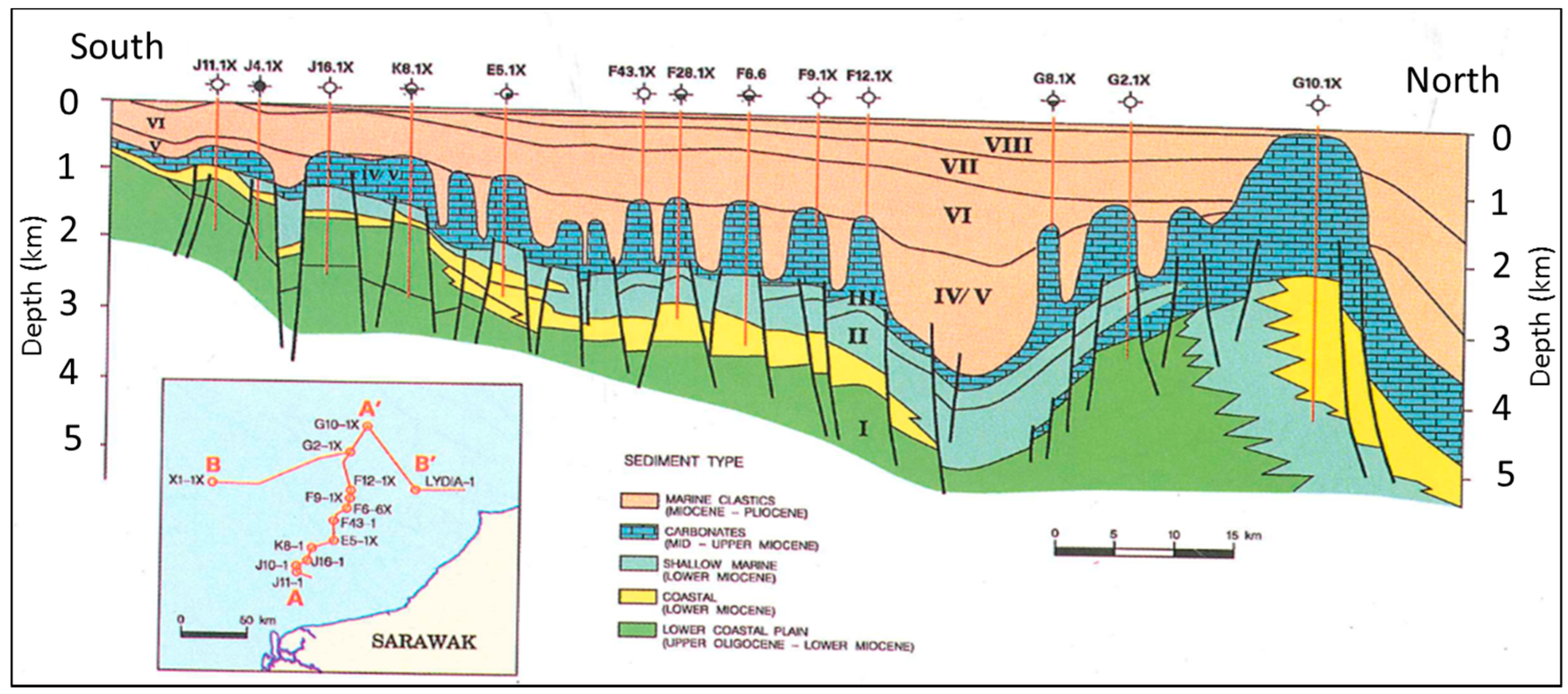
The Sarawak basin is an important hydrocarbon exploration area for Malaysia, with its Middle Miocene pinnacle reefs and platforms of cycle III–IV and with its post-carbonate clastics playing an important role in hydrocarbon exploration; this is shown in Figure 1b. However, cycles I and II pre-carbonate clastics are considered to be the future potential targets. Figure 2 shows the structural trend resulting from normal faults that involve the basement, where the movement was eventually halted by carbonate sedimentation at different times and different platforms [10]. Figure 3 shows the differentiated fields and blocks of the Luconia province, in offshore Sarawak basin, East Malaysia.
2. Database and Methodology
2.1. Database
A 3D data set from the Sarawak Basin is used for diffraction imaging to resolve the small-scale events. The data set provided for this project was unprocessed offset stack data starting from 80 m to 4730 m with an interval of 75 m offset. The 3D data was acquired by Petroleum Geo-Services (PGS). Data acquisition was conducted in 2006 with the configuration of two guns and six streamers resulting in 12 subsurface lines per boat pass. The data recorded length was 5.7 s with a 2 ms sample interval (Table 1).
The reprocessing objective was to obtain better imaging of the carbonates. The processing sequence and parameters were established together with Veritas DGC and Petronas Carigali Malaysia.
2.2. Pre-Processing for Diffraction Enhancement in Real Data Sarawak Basin
The processing is crucial for diffraction imaging as diffraction events are viewed as noise that is suppressed either intentionally or implicitly during processing [11]. Therefore, careful processing is performed, where diffracted events are preserved and where the diffraction behavior is checked for QC at each step.
Figure 4 shows the use of a processing workflow to image the data. Initially, raw data is provided to the processor, in which there is trace editing with the navigation position; later on, these were merged together accordingly. In order to enhance the signal and reduce noise, filtering and gain were applied to the raw data to increase the quality of the data. Q compensation is a data processing technology used for enhancing the resolution of the seismic data; Q is the seismic inelastic attenuation factor or seismic quality factor which measures energy loss as the seismic wave moves. Tau-p is described in terms of slope dt/dx = p and intercept time, and the arrival time is obtained by projecting the slope back to x = 0 where x is the source-receiver distance. Normal moveout (NMO) corrections are applied to the data due to the effect of the distance between the seismic source and the receiver on the arrival time of a reflection in the form of a time increase with offset. Velocity data obtained during NMO correction are used for stacking the data. This stack data were fed into the diffraction separation algorithm using the method below.
2.3. Angle Stacks
Angle stacks provide a means of accessing the amplitude versus offset (AVO) information of the data [12]. These stack data provide a measurement of the reflectivity at a given angle. There are a number of ways to construct angle stacks. In this work, we used the normal moveout corrected common reflection point gathers within constant angle mutes and the incidence angles in order to define the mute estimated from a velocity field.
2.4. Diffraction Separation Methods
One of the best practices and methods for preserving diffraction is the plane-wave destruction (PWD) filter, initially introduced by Claerbout [13] for the characterization of seismic images using the superposition of local plane waves. This PWD filter is based on the plane-wave differential equation, after the original plane-wave destruction filter with the same approximation was found to exhibit poor performance when applied to spatially aliased data, and compared to frequency–distance (F–X) prediction-error filters [14,15]. The plane wave destruction filter, which can be thought of as a time–distance (T–X) analogy of the frequency–distance (F–X) prediction error filter (PEF), originating from a local plane-wave model, is used for characterizing seismic data [15]. Unfortunately, early experiences in applying plane-wave destruction for interpolating spatially aliased data [13], yielded poor results in comparison with the industry standard frequency distance (F–X) prediction-error filters [14]. A workflow which uses the plane wave destruction for diffraction imaging is shown below. Plane-wave destruction of common-offset data may face difficulties extracting diffractions in regions which have a complex geology and velocity variation [16].
Figure 5 shows the work flow employed in the preservation of diffraction by using plane-wave destruction filter. The method is better than Dip Frequency Filtering (DFF) [18]. The regularization condition is applied to both and :
where D is an appropriate roughening operator and Epsilon is a scaling coefficient. The above equation solution is dependent on the initial values of slopes 1 and 2, which should not be equal to each other. It can be extended to the number of the equation with respect to the number of the grid in the data set [19]. However, this equation is used for calculating the slopes for the given data set.
3. Results
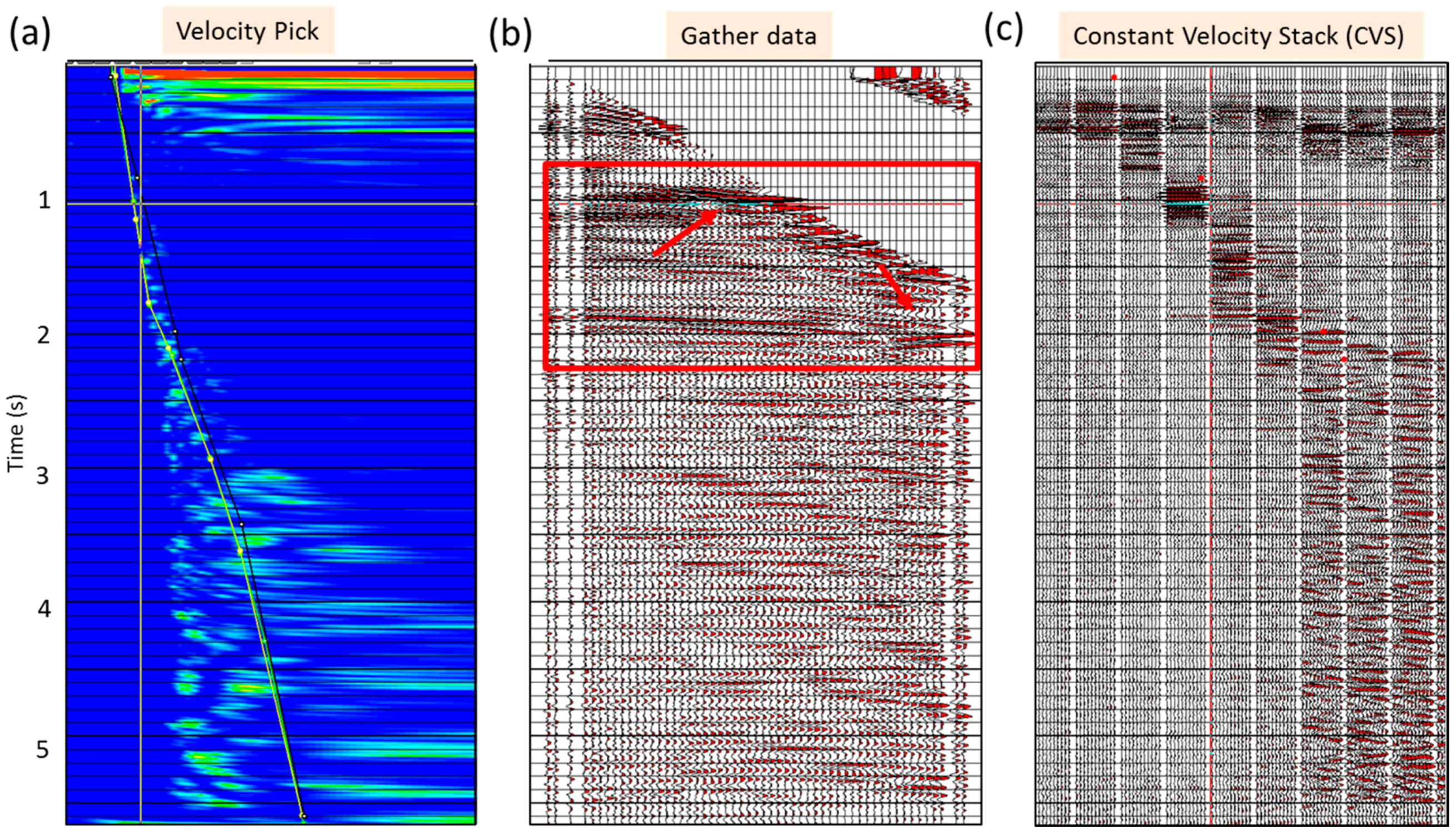
Velocity analysis is a complex and time-consuming task in seismic data processing, and calculating an accurate velocity for depth migration is a geophysicist’s dream. Velocity or stacking velocity can be calculated from normal moveout (NMO), which is the change in arrival time produced by the source and receiver offset. One of the precautions for calculating velocity is to take enough points in the semblance plot; this is because assuming the number of points does not suffice to pick up the velocity, then the moveout of the reflectors will not be straight.
Figure 6a shows velocity picking on the gather semblance plot and Figure 6b shows the gather flattening. After the correct velocity picking, the flattening of the reflector is checked as shown inside red area with red arrows, and this successful picking velocity also helps to improve the velocity model for the stacking of the gather data into the angle and further to full stack data. Figure 6c shows a constant velocity stack (CVS) on the right. Figure 7 is the final results which is come up after NMO correction, the reflectors are flattened by correct picking the velocity as highlighted with red rectangle.
3.1. Effect of Angle Stack on Diffraction
Because angle stacking is designed to measure the reflectivity of a given angle, angle-stacked data are used to observe amplitude versus offset (AVO) for the direct hydrocarbon indicator (DHI) and the inversion in the oil & gas industry. Angle stacking also applies to the general combination of intercept and gradient. These angle stacks usually have near, mid and far angles but an angle stack can consist of more than three angle stacks with a limit of at least 1 degree. For our diffraction studies, a 3 angle stack was performed, as shown in Figure 8. For comparison of only the near and far, the stacking was performed with two angles, 4.5 and 31.5-degree angle stacking, as shown in Figure 9. This shows that a far angle data provides a better diffraction amplitude than a near angle stack data.
As the stacking angle increases, there is a loss of amplitude in the data, as seen in the lower part of the section (Figure 8) but an increase in diffraction response as indicated with a red arrow. Figure 9 is the comparison of the near and far stacked data, in which a diffraction response is not appears in near but the far angle stack show better diffraction preservation. This diffraction would need a larger migration aperture to stack the energy at the flanks of the diffraction to the apex.
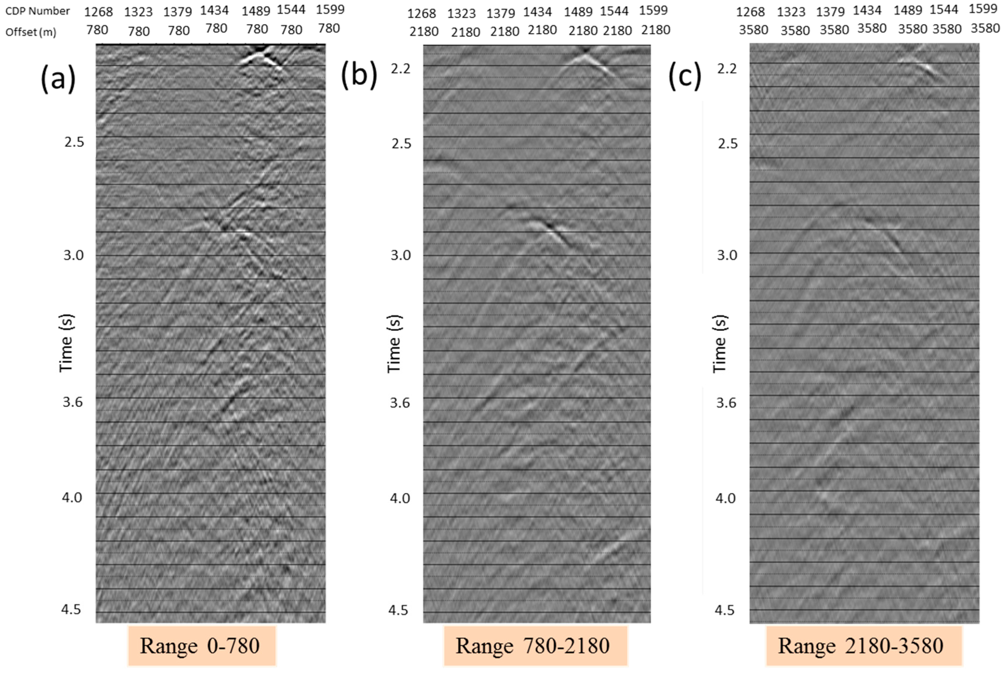
3.2. Effect of Offset Stack on Diffraction
Figure 10 shows the diffraction with offset. Theoretically, the flanks of the diffraction curve are affected by the velocity and time/depth of the point diffractor [18,19]; however, Figure 11 shows that the diffraction also depends on the offset of the data because the near offset data have higher diffraction response than the far offset data. That is the reason behind choosing a zero-offset data for diffractions studies and preservation.
3.3. Separation of Diffraction for High-Resolution Imaging: Real Field Data
Unmigrated offset gather data was provided for this project. Initial processing, including sorting from offset gather to common mid-point (CMP), was performed in order to obtain the stack seismic section. The following procedures were adopted in the sorting process:
- Select a window around the structure with the maximum diffraction response.
- Extract the inline and crossline from the 3D data to obtain a single 2D line.
- The inline was constant over the full length; 810 traces were extracted from the crossline.
- Perform velocity analysis NMO correction.
- Perform offset dependent diffraction enhancement analysis.
- Stack the data for diffraction analysis in the full stack data set.
- Estimate dip components from the data using Equations (1) and (2), as given above.
- Remove the reflections and preserve the diffractions via plane-wave destruction (PWD) filtering [15].
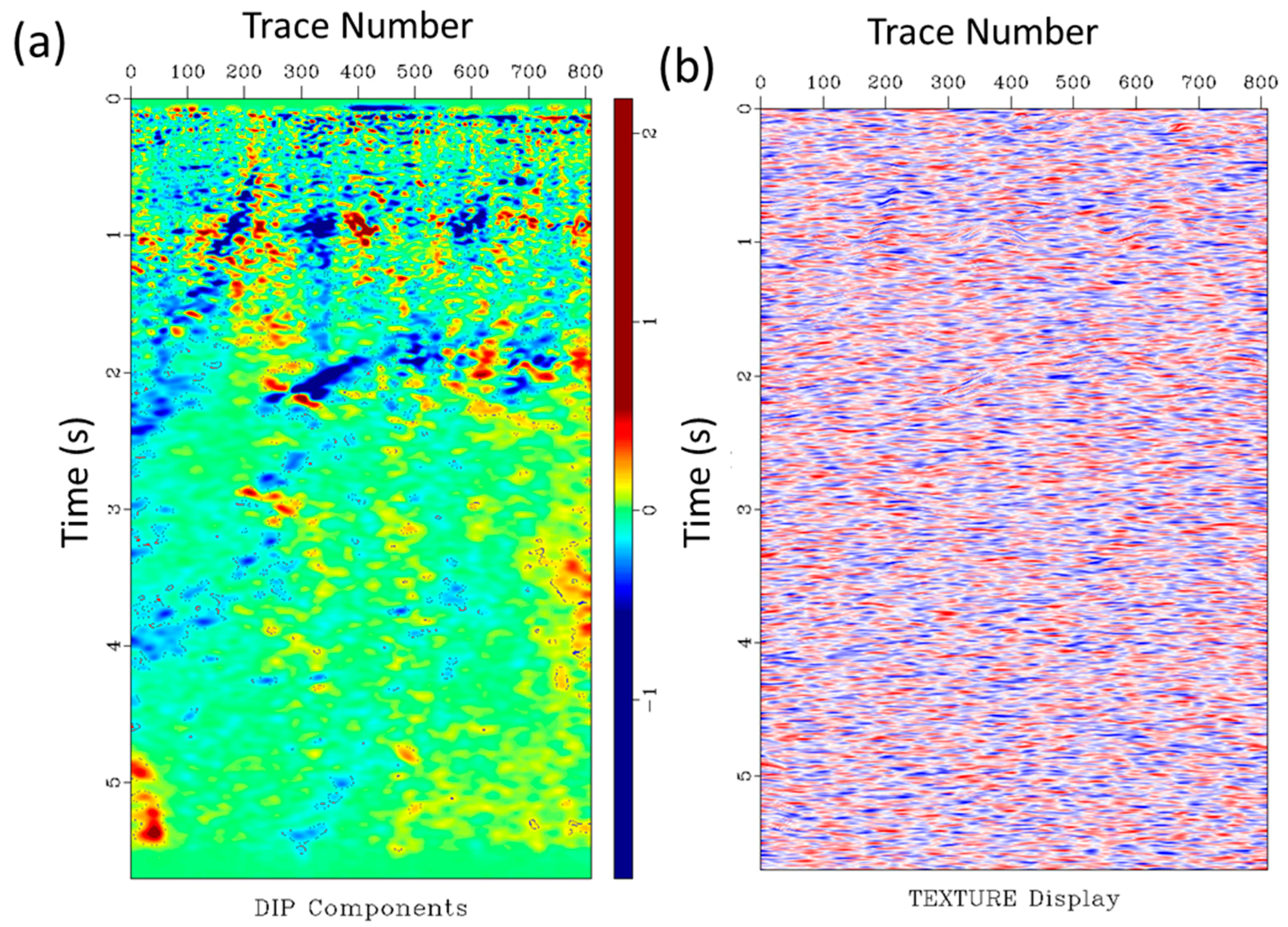
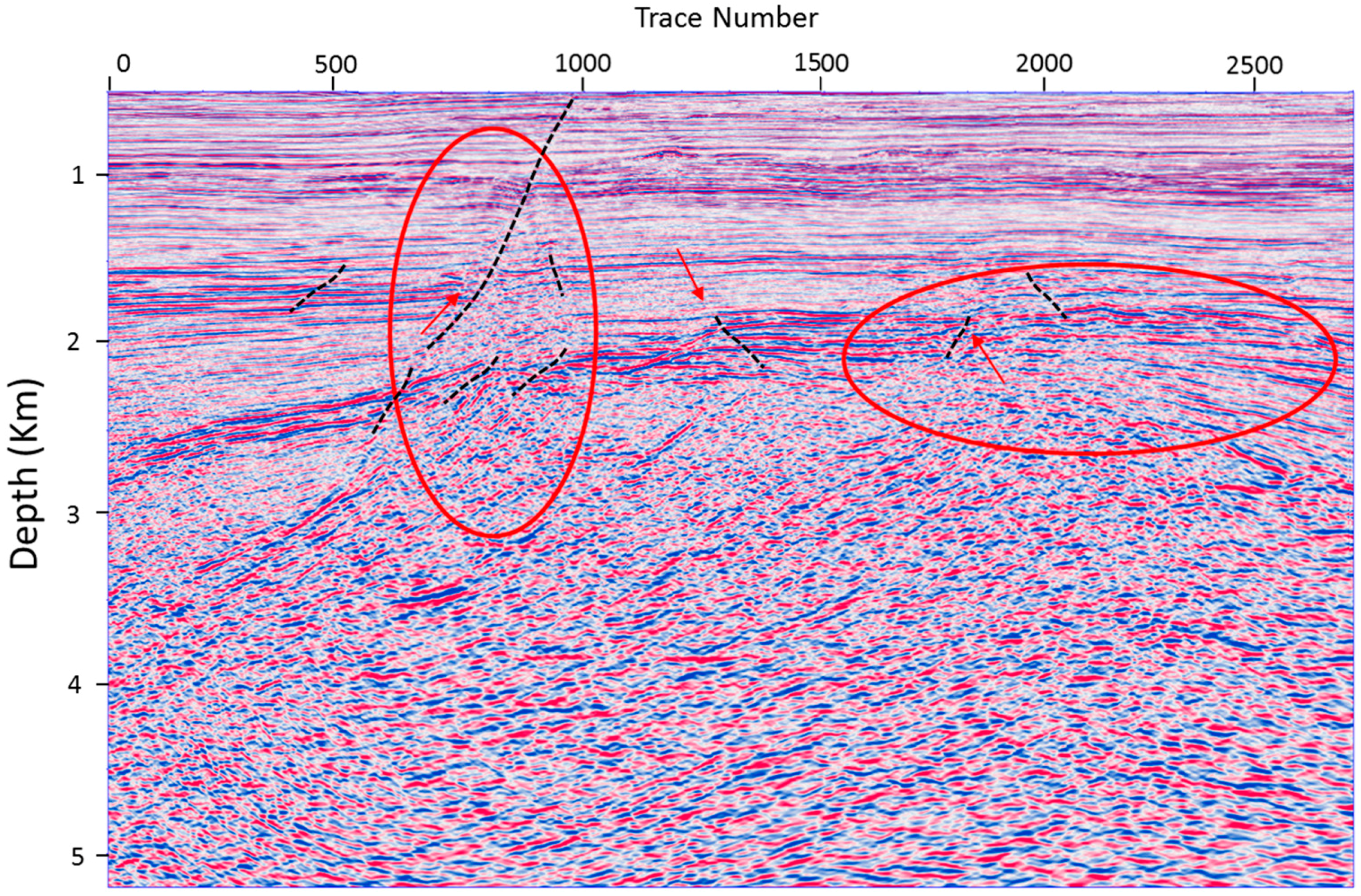
Figure 12 shows a 2D stacked, unmigrated seismic section from a carbonate field in the Sarawak Basin. It was carefully processed using pre-imaging procedures. The diffraction separation method was then extended to preserve the diffractions in the real data. Figure 13a shows the estimated dip components of the data, which help to identify the dipping faults and pinch-outs, while Figure 13b shows the corresponding texture [20] obtained by convolving a field of random numbers with the inverse of the plane-wave destruction filters. The latter was constructed using helical filtering techniques [21,22]. The benefit of texture display is that it helps visualize the local plane features in the data with the dip. Figure 14 shows the separated diffraction that is the input for diffraction imaging. These diffraction data are separately migrated, and they merge with residual data such as reflection migration, as shown in Figure 15. The final migration result includes both diffraction and reflection data, enhancing the resolution of the data. Inside the red circle on the left side, a major fault is imaged and can be interpreted, while in the red circle further on the right side small-scale faults are illuminated after imaging.
4. Conclusions
We present the significance and importance of careful pre-image processing and diffraction imaging in complex Earth-like fractured zones, fault edges, small-scale faults and pinch-outs. The effect of the angle is incorporated into the study as the Zoeppritz equation considers the angle of incidence and not offsets. The offsets with the given velocity field are converted firstly into the angle of incidence and then into Sin square because AVO is analyzed in the Sine square domain. Our research shows that far angle stack data provides better diffraction response than near angle stack.
In processing, plane-wave destruction filters with an improved finite-difference design have an added value for preserving diffraction. These diffraction data contain information regarding the diffracted events which are not recorded in the reflected wave, migrate it separately and merge with the reflected data. In conclusion, it is very useful to consider diffraction in processing and imaging for high-resolution diffraction imaging.
Acknowledgments
The authors are thankful to Universiti Teknologi PETRONAS (UTP), the Geoscience Department and the Centre of Seismic Imaging (CSI) for providing the facilities for this research work. We would also like to thank PETRONAS for funding this work and providing data for research and publication. I would like to say special thanks to my colleague Yaser and Amir Abbas Babasafari for helping me in this research. Finally, our esteemed thanks go to the reviewers of the Geosciences journal who have really helped us to improve the article.
Author Contributions
Yasir Bashir developed the workflow for processing and diffraction separation and applied it to the real seismic data; Deva Prasad Ghosh technically reviewed the work and helped to improve the result; Hammad Tariq Janjuhah performed the geological studies on the area, and Chow Weng Sum reviewed the final results and article technically and wrote the geological aspects of the area.
Conflicts of Interest
The authors declare no conflict of interest.
References
- Popovici, A.M.; Sturzu, I.; Moser, T.J. High Resolution Diffraction Imaging of Small Scale Fractures in Shale and Carbonate Reservoirs; AAPG: Tulsa, OK, USA, 2015. [Google Scholar]
- Krey, T. The significance of diffraction in the investigation of faults. Geophys. Prospect. 2010, 9, 77–92. [Google Scholar] [CrossRef]
- Ogiesoba, O.C.; Klokov, A. Examples of seismic diffraction imaging from the Austin Chalk and Eagle Ford Shale, Maverick Basin, South Texas. J. Petrol. Sci. Eng. 2017, 157, 248–263. [Google Scholar] [CrossRef]
- Ogiesoba, O.C.; Klokov, A. Diffraction Imaging of Lithology and Fluid Saturation in Fault Zones within the Austin Chalk and Eagle Ford Shale, Maverick Basin, South Texas. In Proceedings of the 2015 SEG Annual Meeting, Philadelphia, PA, USA, 18–22 April 2015. [Google Scholar]
- Nowak, E.J.; Imhof, M.G. Diffractor localization via weighted Radon transforms. In SEG Technical Program Expanded Abstracts 2004; Society of Exploration Geophysicists: Denvor, CO, USA, 2004; pp. 2108–2111. [Google Scholar]
- Schwarz, B.; Gajewski, D. Accessing the diffracted wavefield by coherent subtraction. Geophys. J. Int. 2017, 211, 45–49. [Google Scholar] [CrossRef]
- Landa, E.; Keydar, S. Seismic monitoring of diffraction images for detection of local heterogeneities. Geophysics 1998, 63, 1093–1100. [Google Scholar] [CrossRef]
- Alsadi, H.N. Seismic Hydrocarbon Exploration; Springer International Publishing: Basel, Switzerlan, 2017. [Google Scholar]
- Ghosh, D.; Halim, M.F.A.; Brewer, M.; Viratno, B.; Darman, N. Geophysical issues and challenges in Malay and adjacent basins from an E & P perspective. Lead. Edge 2010, 29, 436–449. [Google Scholar]
- Madon, M. Geological setting of Sarawak; Petroleum Geological Resource of Malaysia: Kuala Lumpur, Malaysia, 1999. [Google Scholar]
- Bashir, Y.; Ghosh., D.; Sum, C.W. Detection of Fault and Fracture using Seismic Diffraction and Behavior of Diffraction Hyperbola with Velocity and Time. In Proceedings of the 11th BIMP-EAGA Summit, Langkawi, Malaysia, 28 April 2015. [Google Scholar] [CrossRef]
- Castagna, J.P.; Backus, M.M. Offset-Dependent Reflectivity: Theory and Practice of AVO Analysis; SEG: Tulsa, OK, USA, 1993. [Google Scholar]
- Claerbout, J.F. Earth Soundings Analysis: Processing Versus Inversion, 6th ed.; Blackwell Scientific Publications: London, UK, 1992. [Google Scholar]
- Spitz, S. Seismic trace interpolation in the F-X domain. Geophysics 1991, 56, 785–794. [Google Scholar] [CrossRef]
- Fomel, S. Applications of plane-wave destruction filters. Geophysics 2002, 67, 1946–1960. [Google Scholar] [CrossRef]
- Decker, L.; Klokov, A.; Fomel, S. Comparison of seismic diffraction imaging techniques: Plane wave destruction versus apex destruction. In SEG Technical Program Expanded Abstracts 2013; Society of Exploration Geophysicists: Houston, TX, USA, 2013; pp. 4054–4059. [Google Scholar]
- Decker, L.; Janson, X.; Fomel, S. Carbonate reservoir characterization using seismic diffraction imaging. Interpretation 2015, 3, SF21–SF30. [Google Scholar] [CrossRef]
- Bashir, Y.; Ghosh, D.; Sum, C. Preservation of seismic diffraction to enhance the resolution of seismic data. In SEG Technical Program Expanded Abstracts 2017; Society of Exploration Geophysicists: Houston, TX, USA, 2017; pp. 1038–1043. [Google Scholar]
- Bashir, Y.; Ghosh, D.; Sum, C. Diffraction Amplitude for Fractures Imaging & Hydrocarbon Prediction. J. Appl. Geol. Geophys. 2017, 5, 50–59. [Google Scholar]
- Claerbout, J.; Brown, M. Two-dimensional textures and prediction-error filters. In Proceedings of the 61st EAGE Conference and Exhibition, Helsinki, Finland, 7–11 June 1999. [Google Scholar]
- Claerbout, J. Multidimensional recursive filters via a helix. Geophysics 1998, 63, 1532–1541. [Google Scholar] [CrossRef]
- Fomel, S.; Claerbout, J.F. Multidimensional recursive filter preconditioning in geophysical estimation problems. Geophysics 2003, 6, 577–588. [Google Scholar] [CrossRef]
Figure 1.
(a) Geographical location of the Malaysian Basin and (b) Malay Basin subsurface structure with a cross-section view. The fractured basement can be seen at a depth of 2–5 km, varying with lateral extension [9].
Figure 1.
(a) Geographical location of the Malaysian Basin and (b) Malay Basin subsurface structure with a cross-section view. The fractured basement can be seen at a depth of 2–5 km, varying with lateral extension [9].


Figure 2.
Sarawak basin, an N–S cross-section of the carbonate deposit in central Luconia [10].
Figure 2.
Sarawak basin, an N–S cross-section of the carbonate deposit in central Luconia [10].

Figure 3.
Location map of the study area [10]. The data used in this research is of the Sarawak Basin which is the Lucania Carbonate field.
Figure 3.
Location map of the study area [10]. The data used in this research is of the Sarawak Basin which is the Lucania Carbonate field.

Figure 4.
Processing flow chart (adapted from the PETRONAS report).

Figure 5.
A diffraction separation workflow based on the slope estimation of the data before imaging [17].
Figure 5.
A diffraction separation workflow based on the slope estimation of the data before imaging [17].

Figure 6.
(a) The semblance velocity vs. time plot of the common mid-point (CMP) 1940, (b) absolute offset gather data after picking the velocity, and (c) constant velocity stack (CVS).
Figure 6.
(a) The semblance velocity vs. time plot of the common mid-point (CMP) 1940, (b) absolute offset gather data after picking the velocity, and (c) constant velocity stack (CVS).

Figure 7.
(a) Before normal moveout (NMO) correction, and (b) after NMO correction. The gathers are flattened with the accurate velocity.
Figure 7.
(a) Before normal moveout (NMO) correction, and (b) after NMO correction. The gathers are flattened with the accurate velocity.

Figure 8.
Angle stack seismic data at three different angles (a) Range limited stack data with 4.5 degrees, (b) 22.5 degrees, and (c) 31.5 degrees.
Figure 8.
Angle stack seismic data at three different angles (a) Range limited stack data with 4.5 degrees, (b) 22.5 degrees, and (c) 31.5 degrees.

Figure 9.
Partial stack seismic with: (a) a near angle stack of 4.5 degree which is almost equal to a zero-offset section, and (b) a far angle stack of 31.5 degrees.
Figure 9.
Partial stack seismic with: (a) a near angle stack of 4.5 degree which is almost equal to a zero-offset section, and (b) a far angle stack of 31.5 degrees.

Figure 10.
Multiple offsets gather data shows that shallow data is not recorded in the far offset. (a) range limited stack of 0–780 m, (b) 780–2180 m, and (c) 2180–3580 m.
Figure 10.
Multiple offsets gather data shows that shallow data is not recorded in the far offset. (a) range limited stack of 0–780 m, (b) 780–2180 m, and (c) 2180–3580 m.

Figure 11.
Amplitude decay with offset is recorded at (a) 0 to 780 m, (b) 780 m to 2180 m offsets, and (c) a 2180 m to 3580 m offset stack; the signal–noise ratio and amplitude is stronger in the near offset.
Figure 11.
Amplitude decay with offset is recorded at (a) 0 to 780 m, (b) 780 m to 2180 m offsets, and (c) a 2180 m to 3580 m offset stack; the signal–noise ratio and amplitude is stronger in the near offset.

Figure 12.
Input real seismic data from the Malaysian Basin, processed with careful diffraction processing and stacked before migration: Sarawak Basin, carbonate build-up structure.
Figure 12.
Input real seismic data from the Malaysian Basin, processed with careful diffraction processing and stacked before migration: Sarawak Basin, carbonate build-up structure.

Figure 13.
(a) Estimated dip field of data, and (b) texture computed by convolving field numbers with the inverse of the plane-wave destruction filters.
Figure 13.
(a) Estimated dip field of data, and (b) texture computed by convolving field numbers with the inverse of the plane-wave destruction filters.

Figure 14.
Pre-migrated preserved diffractions following the application of the plane-wave destruction (PWD) filtering on zero-offset data.
Figure 14.
Pre-migrated preserved diffractions following the application of the plane-wave destruction (PWD) filtering on zero-offset data.

Figure 15.
Imaged section, including the preserved diffraction. Faults are resolved and seismic data quality is enhanced.
Figure 15.
Imaged section, including the preserved diffraction. Faults are resolved and seismic data quality is enhanced.


Table 1.
Acquisition summary of the study area in Sarawak basin, East Malaysia.
| Recorded by | PGS Geophysical, Marine Acq |
|---|---|
| Date | 2006 |
| Recorded Length | 5.7 s |
| Sample Rate | 2 ms |
| Recording filter | Low cut: 3 Hz, High cut: 218 Hz |
| Number of sources | 2 |
| Volume of Sources | 3090 Cu. In. Dual Source Flip-flop |
| Pressure | 2000 PSI |
| Source Depth | 6 m |
| Shot Interval | 18.75 m per CSP line |
| Number of Cables | 6 |
| Number of Groups | 384 per Streamer |
| Cable Separation | 75 m |
| Group Interval/length | 12.5 m |
| Cable length | 4800 m |
| Cable Depth | 7 m |
| Near Offset | 80 m |
© 2018 by the authors. Licensee MDPI, Basel, Switzerland. This article is an open access article distributed under the terms and conditions of the Creative Commons Attribution (CC BY) license (http://creativecommons.org/licenses/by/4.0/).
Share and Cite
MDPI and ACS Style
Bashir, Y.; Ghosh, D.P.; Janjuhah, H.T.; Weng Sum, C. Diffraction Enhancement Through Pre-Image Processing: Applications to Field Data, Sarawak Basin, East Malaysia. Geosciences 2018, 8, 74. https://doi.org/10.3390/geosciences8020074
AMA Style
Bashir Y, Ghosh DP, Janjuhah HT, Weng Sum C. Diffraction Enhancement Through Pre-Image Processing: Applications to Field Data, Sarawak Basin, East Malaysia. Geosciences. 2018; 8(2):74. https://doi.org/10.3390/geosciences8020074
Chicago/Turabian StyleBashir, Yasir, Deva Prasad Ghosh, Hammad Tariq Janjuhah, and Chow Weng Sum. 2018. "Diffraction Enhancement Through Pre-Image Processing: Applications to Field Data, Sarawak Basin, East Malaysia" Geosciences 8, no. 2: 74. https://doi.org/10.3390/geosciences8020074
Note that from the first issue of 2016, this journal uses article numbers instead of page numbers. See further details here.