A Transient ElectroMagnetic (TEM) Method Survey in North-Central Coast of Crete, Greece: Evidence of Seawater Intrusion

Abstract
:1. Introduction
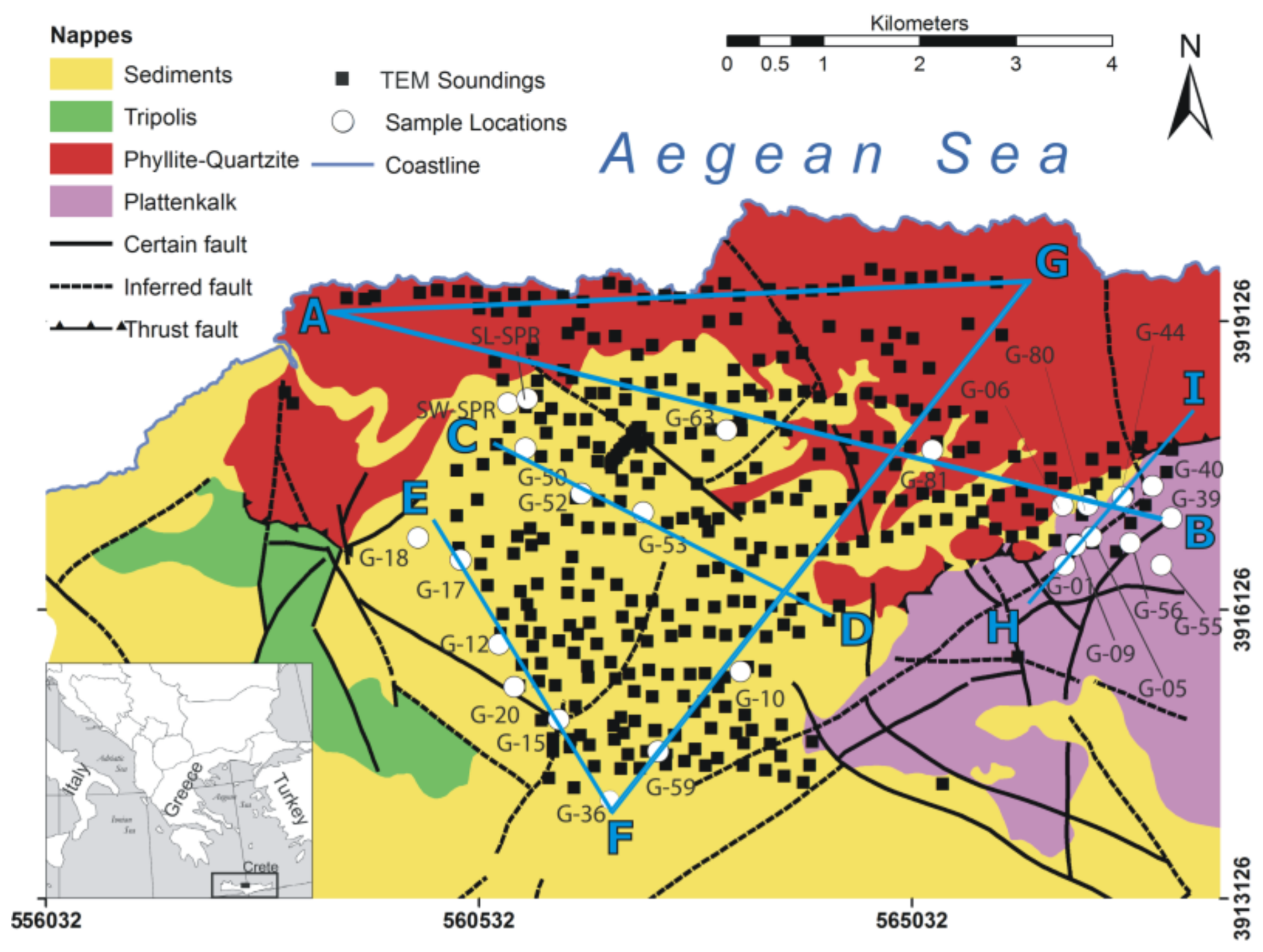
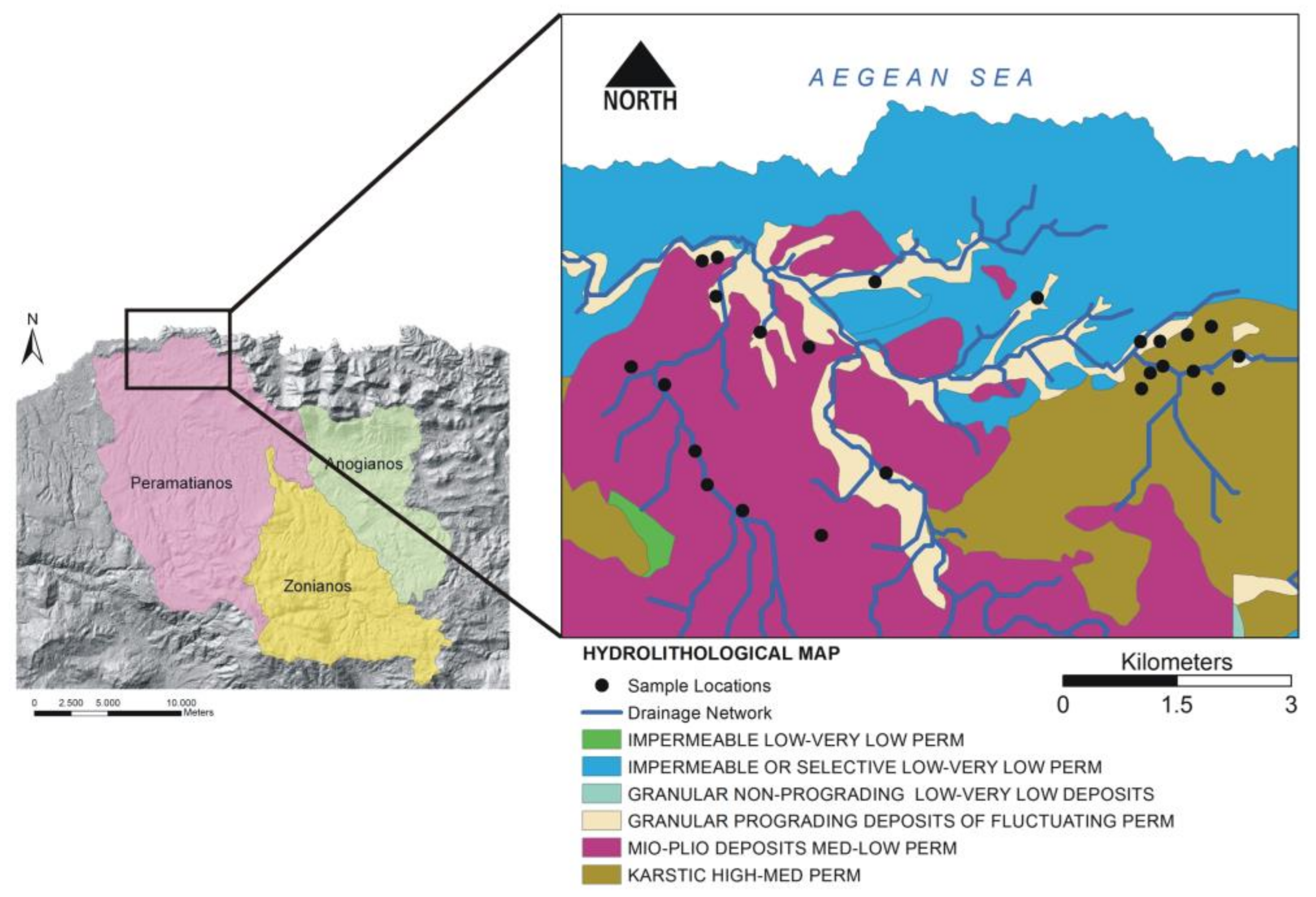
2. The Study Area
2.1. Geological Setting
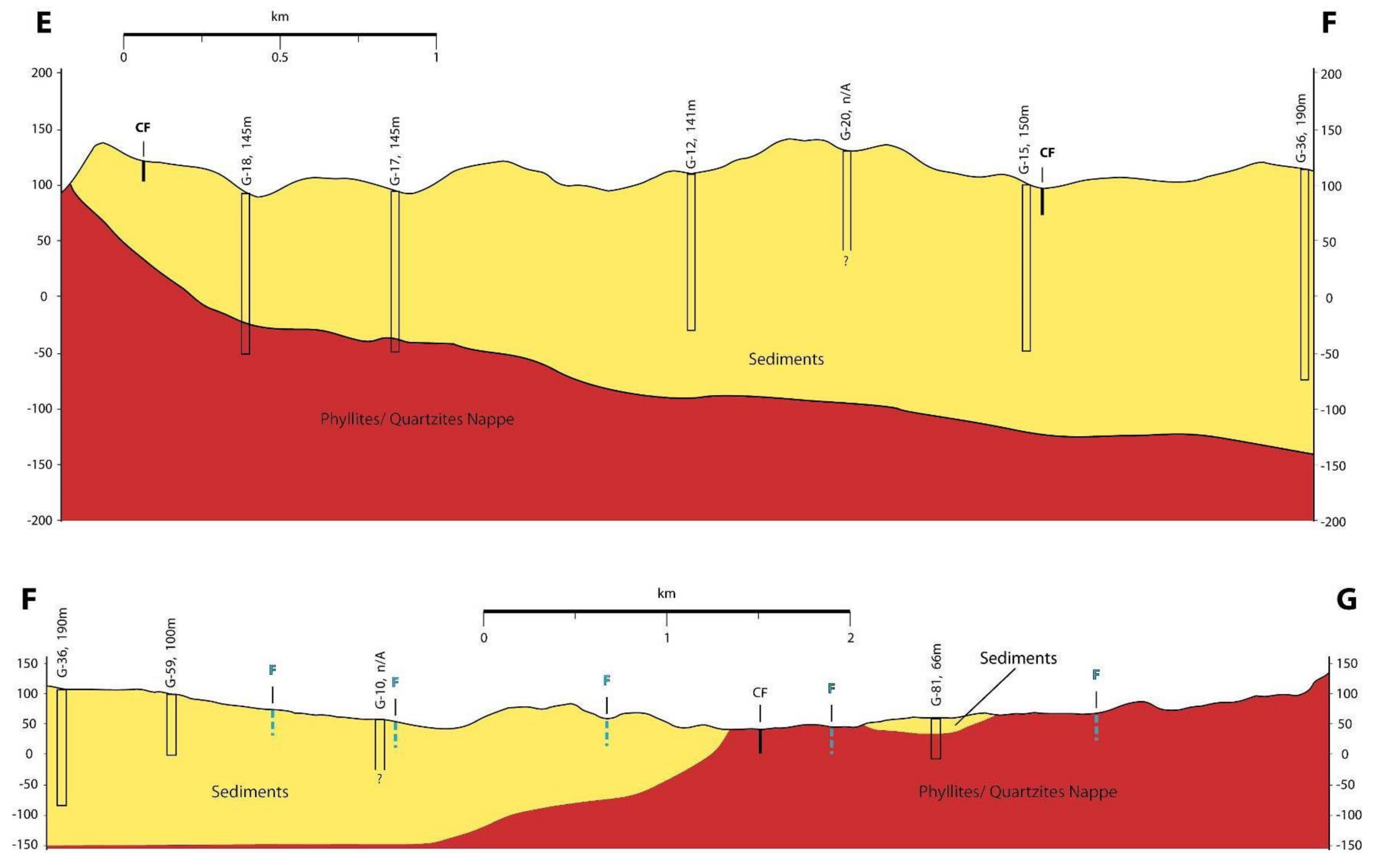
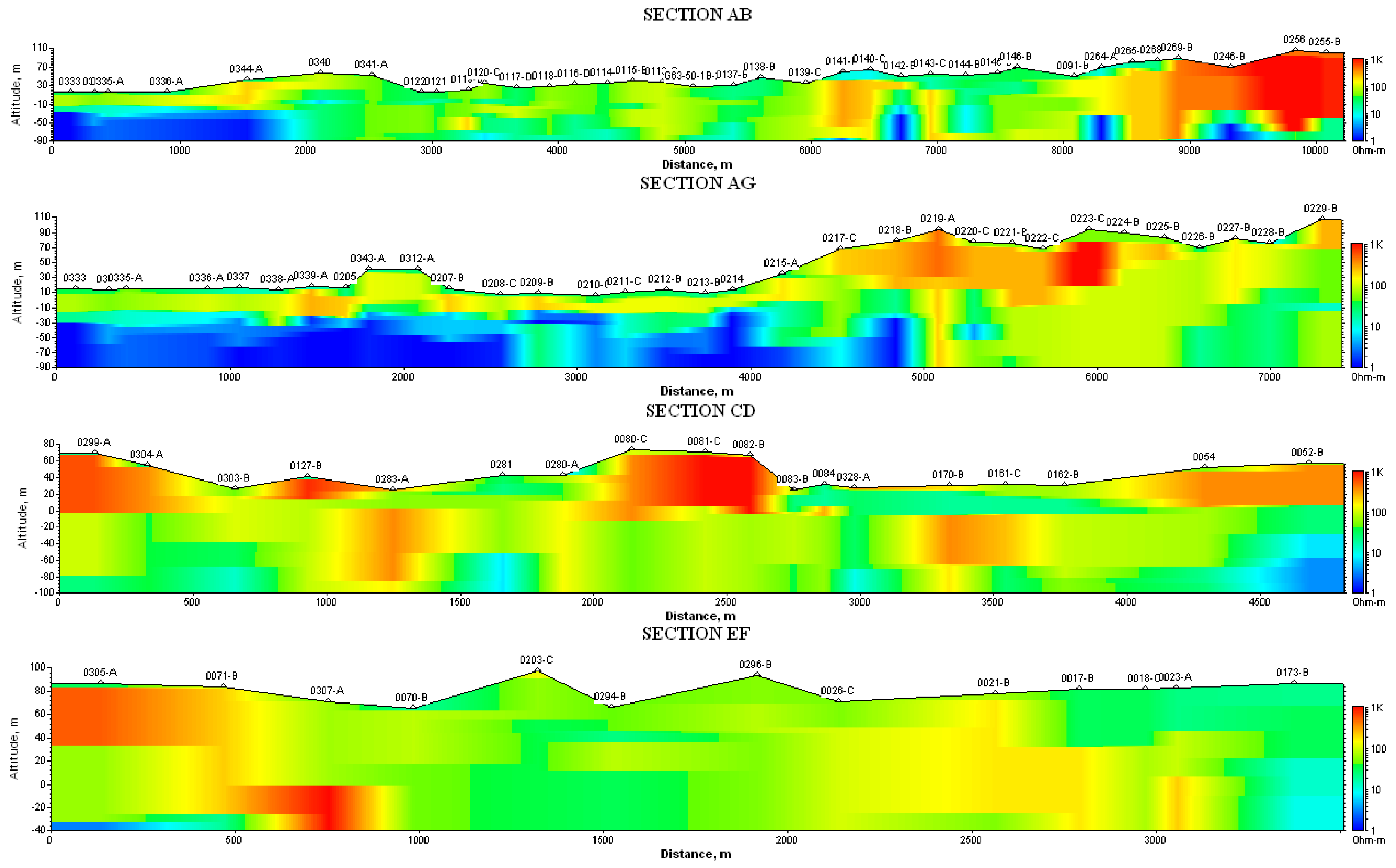
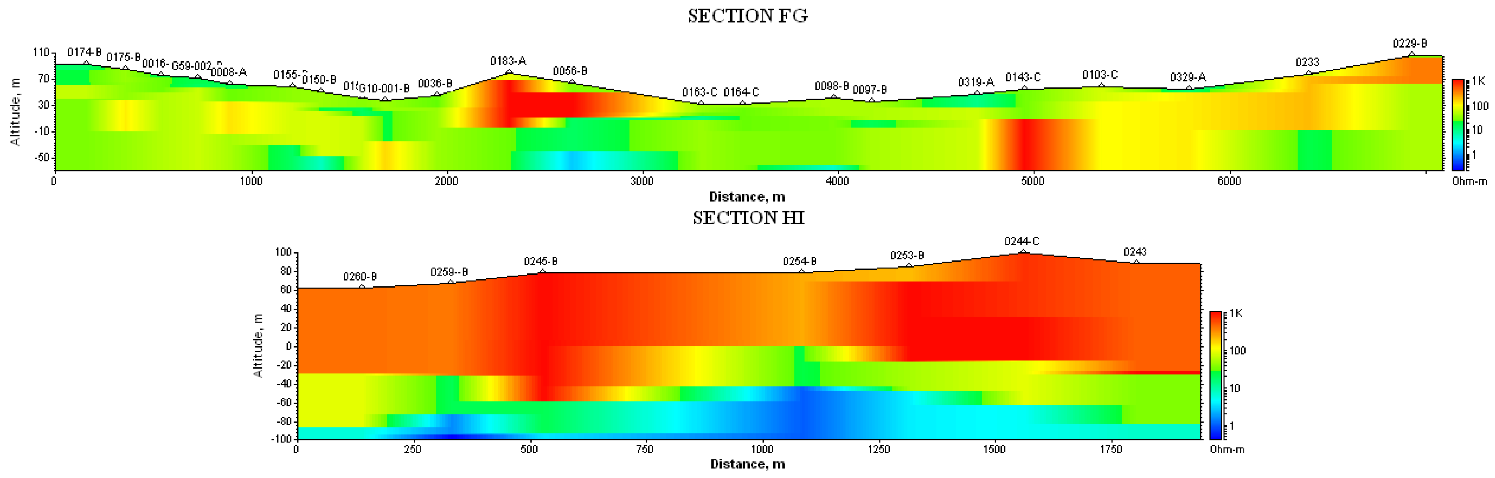
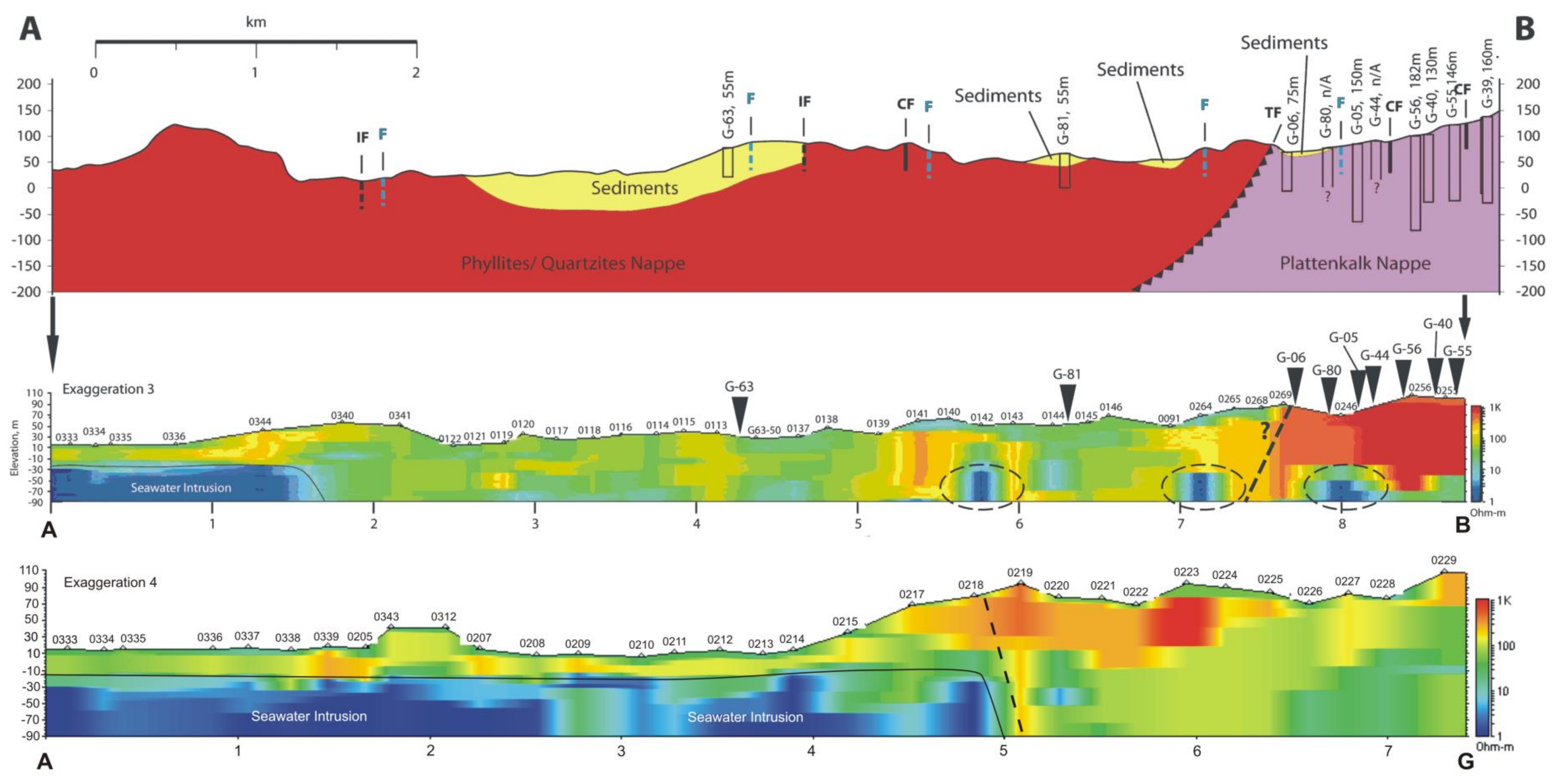
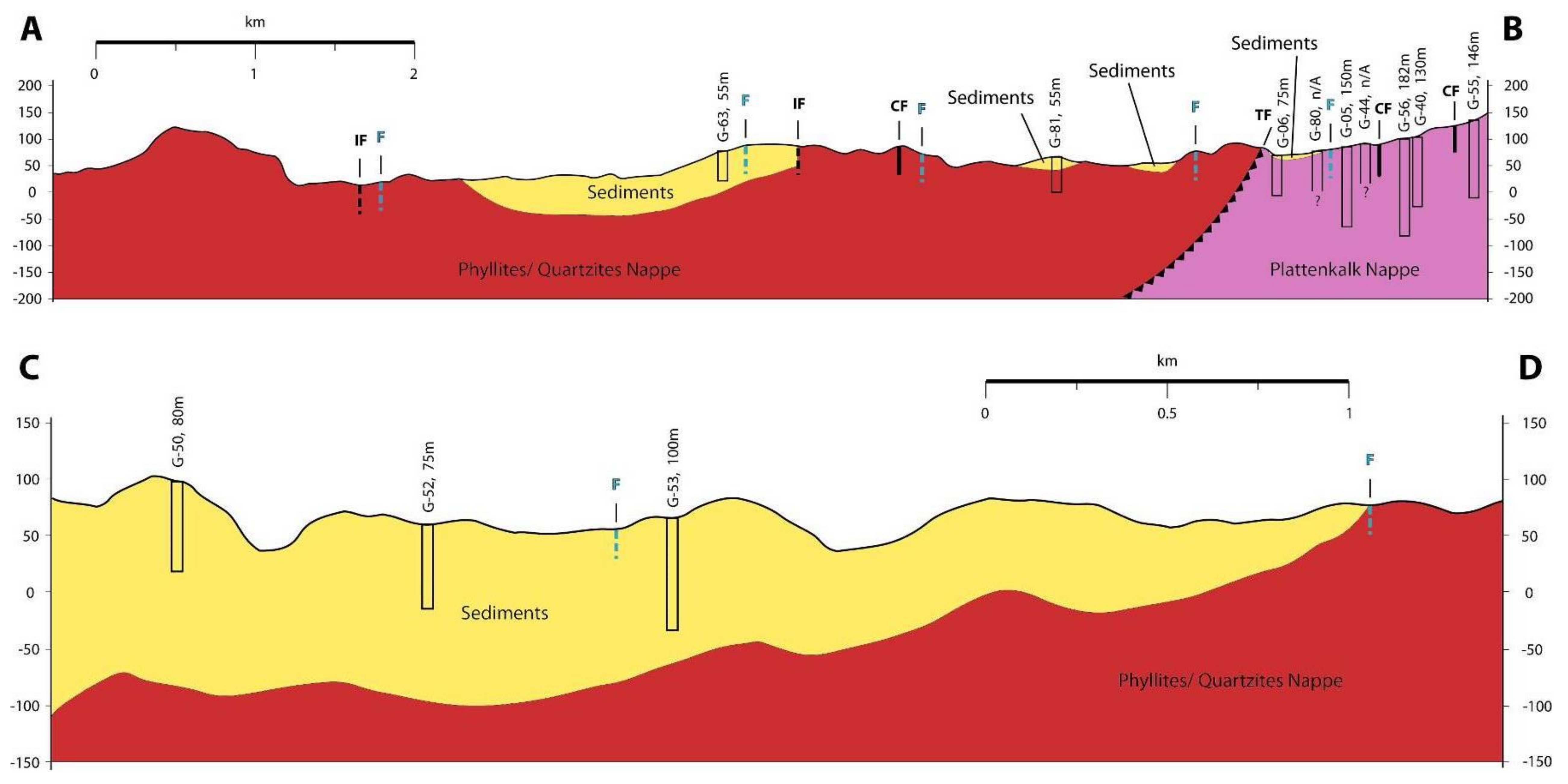
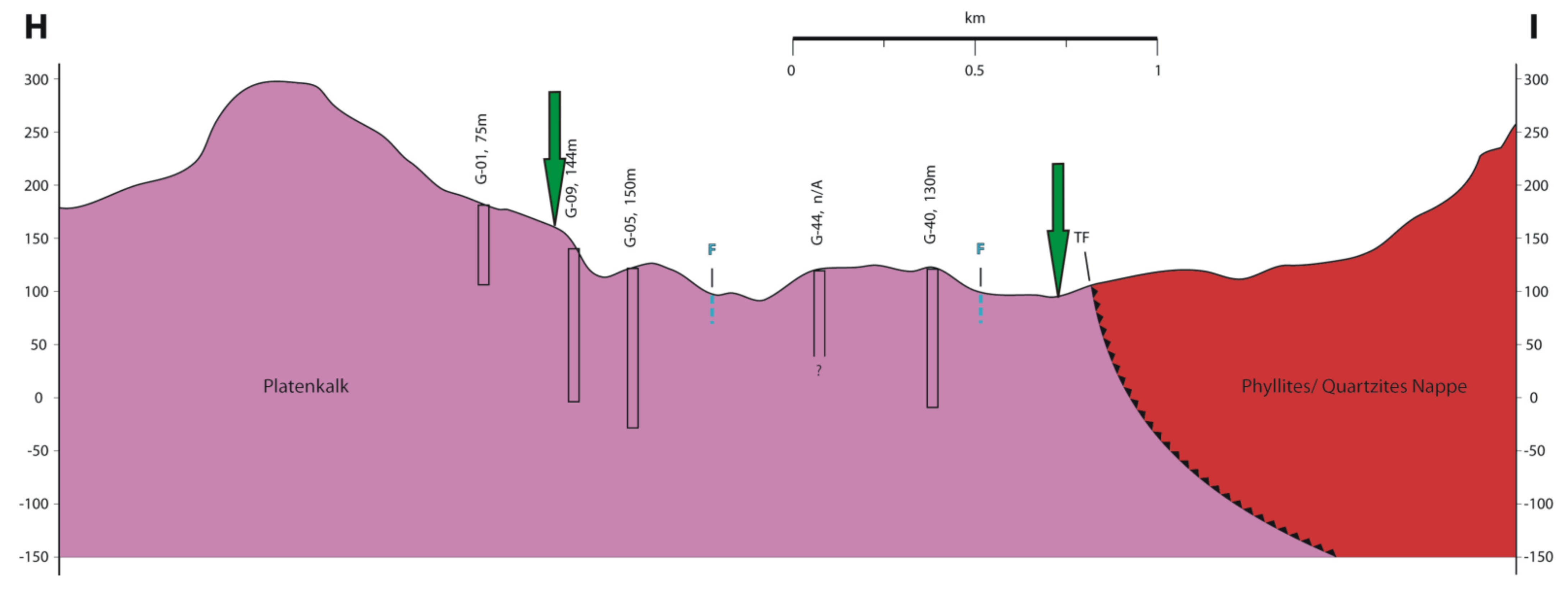
2.2. Geological Cross Sections
3. Methods
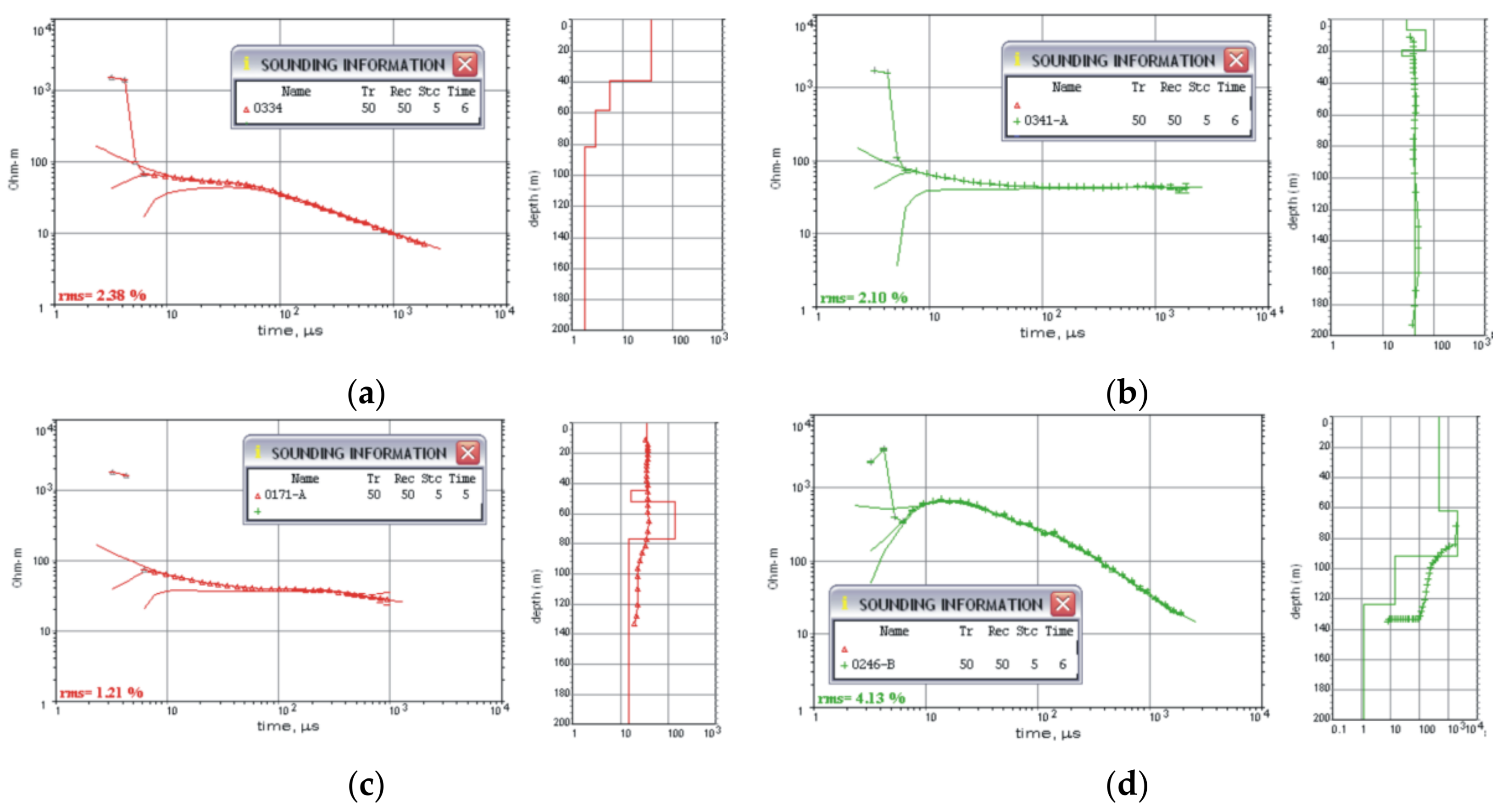
3.1. The TEM Technique
3.2. Geochemical Analyses
4. Results
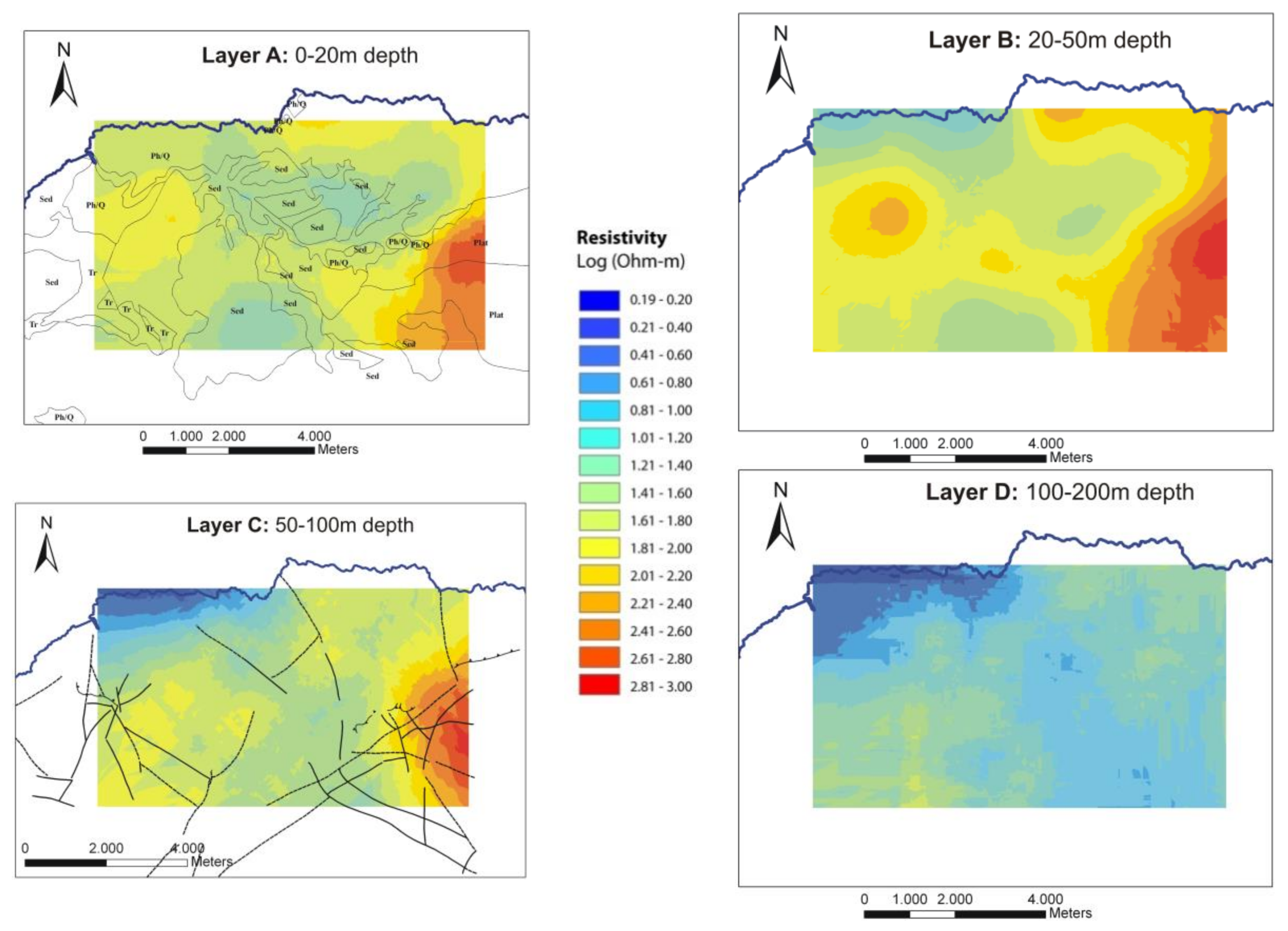
4.1. TEM Approach
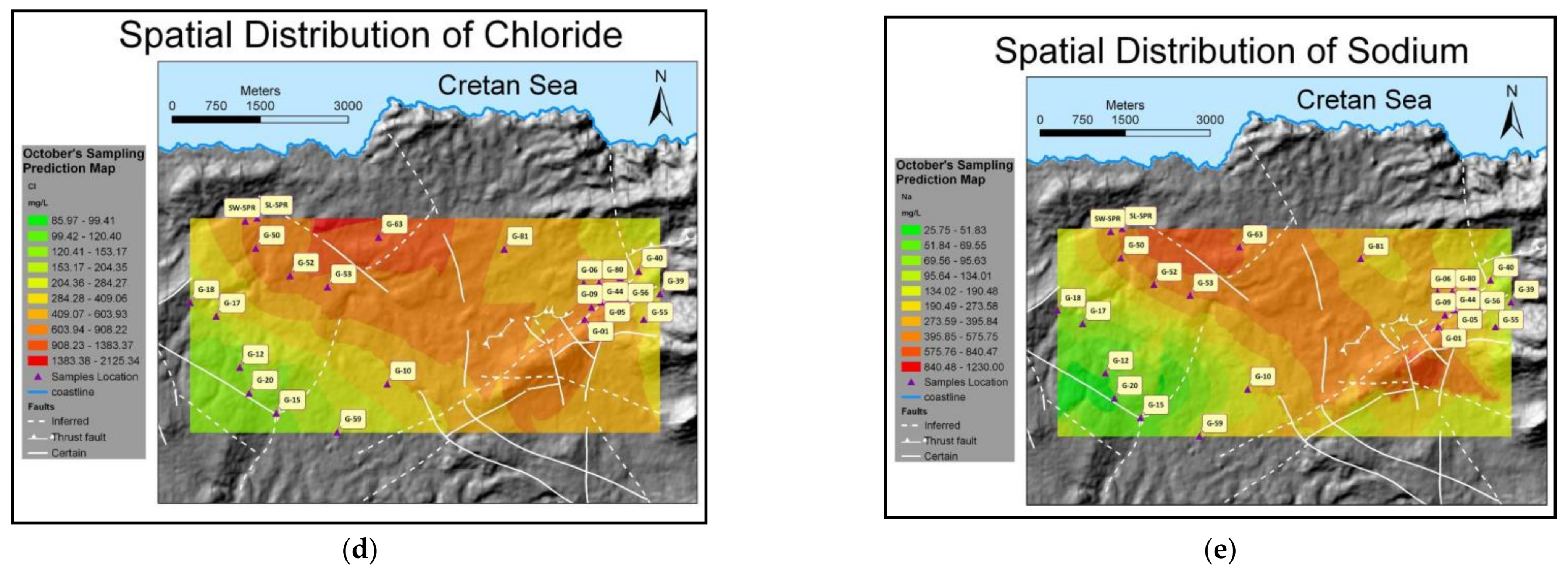
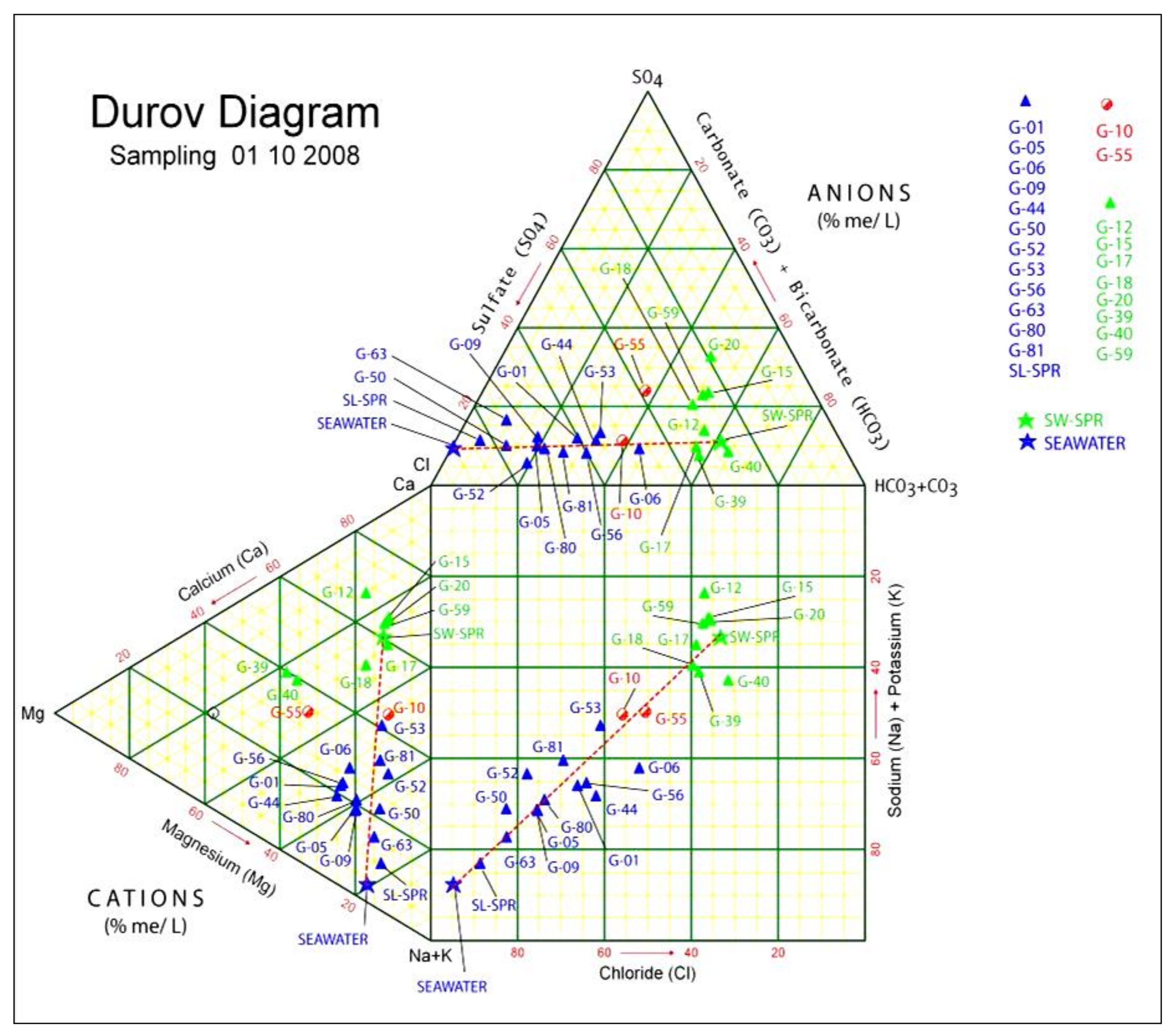
4.2. Water Quality
5. Data Interpretation and Discussion
6. Conclusions
Acknowledgments
Author Contributions
Conflicts of Interest
References
- Meju, M.A.; Fenning, P.J.; Hawkins, T.R.W. Evaluation of small-loop transient electromagnetic soundings to locate the Sherwood Sandstone aquifer and confining formations at well sites in the Vale of York, England. J. Appl. Geophys. 2000, 44, 217–236. [Google Scholar] [CrossRef]
- Guérin, R.; Descloitres, M.; Coudrain, A.; Talbi, A.; Gallaire, R. Geophysical surveys for identifying saline groundwater in the semi-arid region of the central Altiplano, Bolivia. Hydrol. Process. 2001, 15, 3287–3301. [Google Scholar] [CrossRef]
- Danielsen, J.E.; Auken, E.; Jorgensen, F.; Sondergaard, V.; Sorensen, K.I. The application of the transient electromagnetic method in hydrogeophysical surveys. J. Appl. Geophys. 2003, 53, 181–198. [Google Scholar] [CrossRef]
- Metwaly, M.; Khalil, M.; Al-Sayed, E.S.; Osman, S. A hydrogeophysical study to estimate water seepage from northwestern Lake Nasser, Egypt. J. Geophys. Eng. 2006, 3, 21–27. [Google Scholar] [CrossRef]
- Soupios, P.; Kalisperi, D.; Kanta, A.; Kouli, M.; Barsukov, P.; Vallianatos, F. Coastal aquifer assessment based on geological and geophysical survey, NW Crete, Greece. J. Environ. Earth Sci. 2010, 61, 63–77. [Google Scholar] [CrossRef]
- Mills, T.; Hoekstra, P.; Blohm, M.; Evans, L. Time domain electromagnetic soundings for mapping sea-water intrusion in Monterey County, California. Ground Water 1988, 26, 771–782. [Google Scholar] [CrossRef]
- Chen, C.-S. TEM Investigations of Aquifers in the Southwest Coast of Taiwan. Ground Water 1999, 37, 890–896. [Google Scholar] [CrossRef]
- Kafri, U.; Goldman, M.; Lang, B. Detection of subsurface brines, freshwater bodies and the interface configuration in between by the Time Domain Electromagnetic (TDEM) method in the Dead Sea rift. Israel J. Environ. Geol. 1977, 31, 42–49. [Google Scholar] [CrossRef]
- Papadopoulos, I.; Tsourlos, P.; Karmis, P.; Vargemezis, G.; Tsokas, G.N. A TDEM survey to define local hydrogeological structure in Anthemountas Basin, N. Greece. J. Balkan Geophys. Soc. 2004, 7, 1–11. [Google Scholar]
- Kontar, E.A.; Ozorovich, Y.R. Geo-electromagnetic survey of the fresh/salt water interface in the coastal southeastern Sicily. Cont. Shelf Res. 2006, 26, 843–851. [Google Scholar] [CrossRef]
- Kanta, A.; Soupios, P.; Barsukov, P.; Kouli, M.; Vallianatos, F. Aquifer characterization using shallow geophysics in the Keritis Basin of Western Crete, Greece. Environ. Earth Sci. 2013, 70, 2153–2165. [Google Scholar] [CrossRef]
- Herckenrath, D.; Odlum, N.; Nenna, V.; Knight, R.; Auken, E.; Bauer-Gottwein, P. Calibrating a Salt Water Intrusion Model with Time-Domain Electromagnetic Data. Ground Water 2013, 51, 385–397. [Google Scholar] [CrossRef] [PubMed]
- Trabelsi, F.; Mammou, A.B.; Tarhouni, J.; Piga, C.; Ranieri, G. Delineation of saltwater intrusion zones using the time domain electromagnetic method: The Nabeul-Hammamet coastal aquifer case study (NE Tunisia). Hydrol. Process. 2013, 27, 2004–2020. [Google Scholar] [CrossRef]
- Gonçalves, R.; Farzamian, M.; Monteiro Santos, F.A.; Represas, P.; Mota Gomes, A.; Lobo de Pina, A.F.; Almeida, E.P. Application of Time-Domain Electromagnetic Method in Investigating Saltwater Intrusion of Santiago Island (Cape Verde). Pure Appl. Geophys. 2017, 174, 4171–4182. [Google Scholar] [CrossRef]
- Sanchez-Martos, F.; Pulido-Bosch, A.; Molina-Sanchez, L.; Vallejos-Izquierdo, A. Identification of the origin of salinization in groundwater using minor ions (Lower Andarax, Southeast Spain). Sci. Total Environ. 2002, 297, 43–58. [Google Scholar] [CrossRef]
- Perry, E.; Velazquez-Oliman, G.; Marin, L. The hydrogeochemistry of the karst aquifer system of the northern Yucatan Peninsula, Mexico. Int. Geol. Rev. 2002, 44, 191–221. [Google Scholar] [CrossRef]
- Kalisperi, D.; Soupios, P.; Kouli, M.; Barsukov, P.; Kershaw, S.; Collins, P.; Vallianatos, F. Coastal aquifer assessment using geophysical methods (TEM, VES), case study: Northern Crete, Greece. In Proceedings of the 3rd IASME International Conference on Geology and Seismology GES ’09, Cambridge, UK, 24–26 February 2009. [Google Scholar]
- Kalisperi, D. Assessment of Groundwater Resources in the North-Central Coast of Crete, Greece Using Geophysical and Geochemical Methods. Ph.D. Thesis, Brunel University, London, UK, 2009. [Google Scholar]
- Sdao, F.; Parisi, P.; Kalisperi, D.; Pascale, S.; Soupios, P.; Lydakis-Simantiris, N.; Kouli, M. Geochemistry and quality of the groundwater from the karstic and coastal aquifer of Geropotamos River Basin at north-central Crete, Greece. Environ. Earth Sci. 2012, 67, 1145–1153. [Google Scholar] [CrossRef]
- Institute of Geology and Mineral Exploration (IGME). Geological Map of Greece, Perama sheet, Scale: 1:50,000; IGME: Athens, Greece, 1991. [Google Scholar]
- Chatzaras, V.; Xypolias, P.; Doutsos, T. Exhumation of high-pressure rocks under continuous compression: A working hypothesis for the southern Hellenides (central Crete, Greece). Geol. Mag. 2006, 143, 859–876. [Google Scholar] [CrossRef]
- Fassoulas, C. Field Guide to the Geology of Crete; Natural History Museum of Crete Publ.: Heraklion, Greece, 2000; ISBN 960-367-008-1.
- Kilias, A.; Fassoulas, C.; Mountrakis, D. Tertiary extension of continental crust and uplift of Psiloritis metamorphic core complex in the central part of the Hellenic arc (Crete, Greece). Geol. Rundsch. 1994, 83, 417–430. [Google Scholar]
- Fassoulas, C.; Kilias, A.; Mountrakis, D. Post-nappe stacking extension and exhumation of the HP/LT rocks in the island of Crete, Greece. Tectonics 1994, 13, 127–138. [Google Scholar] [CrossRef]
- Knithakis, M. Hydrogeological Investigation of Rethymnon Region (Prefecture of Rethymnon); Institute of Geological and Mineralogical Investigations (IGME): Rethymnon, Greece, 1995. (In Greek) [Google Scholar]
- Region of Crete. Study of Water Resources Management of Crete; Region of Crete: Heraklion, Greece, 1999. (In Greek)
- Zarris, D. Water Supply Masterplan of Municipality of Geropotamos; Municipality of Geropotamos: Perama, Crete, Greece, 2008. (In Greek)
- Nabighian, M.N.; Macnae, J.C. Time domain electromagnetic prospecting methods. In Electromagnetic Methods in Applied Geophysics; Nabighian, M.N., Ed.; Society of Exploration Geophysics: Denver, CO, USA, 1991; Volume 2, pp. 427–520. ISBN 978-1-56080-022-4. [Google Scholar]
- Barsukov, P.O.; Fainberg, E.B.; Khabensky, E.O. FAST technique: Methodology and examples. In Electromagnetic Sounding of the Earth’s Interior: Theory, Modeling, Practice, 2nd ed.; Spichak, V.V., Ed.; Elsevier: Amsterdam, The Netherlands; Cambridge, UK; Atlanta, GA, USA, 2015; Chapter 3; pp. 47–78. ISBN 978-0-44463-554-9. [Google Scholar]
- Yalçin, H.; Koç, T.; Pamuk, V. Hydrogen and bromine production from concentrated sea-water. Int. J. Hydrogen Energy 1997, 22, 967–970. [Google Scholar] [CrossRef]
- Appelo, C.A.J.; Postma, D. Geochemistry, Groundwater and Pollution, 2nd ed.; CRC Press: Boca Raton, FL, USA, 2005; ISBN 978-0-415-36428-7. [Google Scholar]
- Babiker, I.S.; Mohamed, A.A.; Hiyama, T. Assessing groundwater quality using GIS. Water Resour. Manag. 2007, 21, 699–715. [Google Scholar] [CrossRef]
- World Health Organization (WHO). Guidelines for Drinking Water Quality, 4th ed.; World Health Organization: Geneva, Switzerland, 2011. [Google Scholar]
- Hermans, T.; Irving, J. Facies discrimination with electrical resistivity tomography using a probabilistic methodology: Effect of sensitivity and regularization. Near Surf. Geophys. 2017, 15, 13–25. [Google Scholar]


| Post-Alpine Rocks | Quaternary Sediments |
| ||
| Neogene Sediments | ||||
| Alpine and Pre-Alpine Rocks | Upper nappes | LP-HT metamorhosed | Uppermost nappe | |
| thrust fault | ||||
| unmetamorphosed | Pindos nappe | |||
| thrust fault | ||||
| LP-LT metamorhosed | Tripolis nappe | |||
| major thrust fault | ||||
| Lower nappes | HP-LT metamorphosed | Phyllite-Quartzite nappe |
| |
| thrust fault | ||||
| Trypali nappe (only in western Crete) | ||||
| thrust fault | ||||
| Plattenkalk nappe |
| |||
| Rock Material | Resistivity (Ω·m) | |
|---|---|---|
| Quaternary sediments |
| 100–500 |
| Neogene sediments | ||
| Phyllite/Quartzite nappe |
| 100–300 |
| Plattenkalk nappe |
| >1000 |
| Fresh water | 20–40 | |
| Affected Fresh water | 10–20 | |
| Brackish water | 0.1–10 | |
© 2018 by the authors. Licensee MDPI, Basel, Switzerland. This article is an open access article distributed under the terms and conditions of the Creative Commons Attribution (CC BY) license (http://creativecommons.org/licenses/by/4.0/).
Share and Cite
Kalisperi, D.; Kouli, M.; Vallianatos, F.; Soupios, P.; Kershaw, S.; Lydakis-Simantiris, N. A Transient ElectroMagnetic (TEM) Method Survey in North-Central Coast of Crete, Greece: Evidence of Seawater Intrusion. Geosciences 2018, 8, 107. https://doi.org/10.3390/geosciences8040107
Kalisperi D, Kouli M, Vallianatos F, Soupios P, Kershaw S, Lydakis-Simantiris N. A Transient ElectroMagnetic (TEM) Method Survey in North-Central Coast of Crete, Greece: Evidence of Seawater Intrusion. Geosciences. 2018; 8(4):107. https://doi.org/10.3390/geosciences8040107
Chicago/Turabian StyleKalisperi, Despina, Maria Kouli, Filippos Vallianatos, Pantelis Soupios, Stephen Kershaw, and Nikos Lydakis-Simantiris. 2018. "A Transient ElectroMagnetic (TEM) Method Survey in North-Central Coast of Crete, Greece: Evidence of Seawater Intrusion" Geosciences 8, no. 4: 107. https://doi.org/10.3390/geosciences8040107