Airflow Dynamics over a Beach and Foredune System with Large Woody Debris


1
Hakai Institute, P.O. Box 309, Heriot Bay, BC V0P 1H0, Canada
2
Department of Geography, University of Victoria, Victoria, BC V8P 5C2, Canada
3
School of Geographical Sciences & Urban Planning & School of Earth & Space Exploration, Arizona State University, Tempe, AZ 85287-5302, USA
4
Earth, Environmental and Geographic Sciences, The University of British Columbia|Okanagan, Kelowna, BC V1V 1V7, Canada
*
Author to whom correspondence should be addressed.
Geosciences 2018, 8(5), 147; https://doi.org/10.3390/geosciences8050147
Submission received: 6 March 2018
/
Revised: 18 April 2018
/
Accepted: 20 April 2018
/
Published: 24 April 2018
(This article belongs to the Special Issue Aeolian Processes and Geomorphology)
Abstract
:Airflow dynamics over beach-foredune systems can be complex. Although a great deal is known about the effects of topographic forcing and vegetation cover on wind-field modification, the role of large woody debris (LWD) as a roughness element and modifier of boundary layer flow is relatively understudied. Individual pieces of LWD are non-porous elements that impose bluff body effects and induce secondary flow circulation that varies with size, density, and arrangement. Large assemblages of LWD are common on beaches near forested watersheds and collectively have a degree of porosity that increases aerodynamic roughness in ways that are not fully understood. A field study on a mesotidal sandy beach with a scarped foredune (Calvert Island, British Columbia, Canada) shows that LWD influences flow patterns and turbulence levels. Overall mean and fluctuating energy decline as flow transitions across LWD, while mean energy is converted to turbulent energy. Such flow alterations have implications for sand transport pathways and resulting sedimentation patterns, primarily by inducing deposition within the LWD matrix.
1. Introduction
Natural roughness elements (e.g., plants, rocks, wrack, logs) protrude into the near-surface flow field, increasing aerodynamic drag and extracting momentum from the wind as well as acting as a physical barrier to aeolian sediment transport [1,2,3,4,5]. There are many studies on the effects of porous and pliable roughness elements (i.e., grassy vegetation) on flow interactions and sediment transport over coastal foredunes [6,7,8,9,10,11,12,13], as well as around discrete, artificial non-porous roughness elements [11,14,15,16] and roughness arrays [17,18,19]. However, there remains a gap in understanding as to how natural non-porous objects, like fallen trees and large woody debris (LWD), affect flow and sedimentation on and in front of coastal foredunes [3,13,14,20].
Flow interactions around isolated, non-porous objects with simple shapes are well-studied and relatively predictable [3,16,21,22,23,24,25] (Figure 1), although the resulting topographic changes are less well understood [15]. Unidirectional horizontal flow around a three-dimensional cylinder (most closely representing an upright tree stump) is characterized by flow separation, the creation of horseshoe vortices extending downwind near the surface, and flow reversals in the lee of the object [15]. Lee flow reversals create an area of converging flow with reduced velocity where shadow dunes form [16,26,27]. McKenna Neuman and Bédard [15] demonstrated that scour, caused by flow acceleration around the sides of the object, migrates windward as minor slope failures. Horseshoe vortices develop as the scour region grows and converges, forming an erosional horseshoe-shaped trough [15,16]. Leenders et al. [28] measured a similar increase in wind speed around the base of single tree trunks.
Research on arrays of non-porous roughness elements has revealed a complex relationship between flow characteristics, sediment transport, and roughness density [17,19,30,31] Uniform roughness array densities >44% (based on spacing pattern) can produce skimming flow [5,22] (Figure 2) that has been shown to reduce the potential for sediment transport downwind of the array, in contrast to isolated roughness elements that have localized influences [3].
Examples of the effects of LWD on aeolian sand transport and erosion/deposition patterns on beaches include extensive upwind and lateral horseshoe basal scour (cf., [15]), which is common for highly exposed elements (Figure 3). However, accumulations of LWD in dense matrices are also common (Figure 4). Variations in LWD matrix shape, size, structure, density, orientation to incoming flow, height above the surface, and apparent porosity create complex flow-form interactions that alter flow characteristics and sediment transport pathways in unpredictable ways. Because of these effects, predicting flow patterns and sand supply to foredune systems laden with LWD becomes increasingly difficult. To date, there is no published research to quantify the impacts of a LWD matrix on airflow in the vicinity of a coastal foredune.
The overall purpose of this study was to improve our understanding of the effects of LWD on near-surface airflow fronting a coastal foredune. The approach was to study the aggregate effect of the LWD deposit, rather than the properties and flow dynamics around individual roughness elements. Three-dimensional airflow and turbulence properties were characterized during sand transport events along shore-perpendicular transects with and without LWD. This paper examines specifically the influence of a recently emplaced LWD matrix on the flow dynamics fronting an established, scarped foredune. On-going research is addressing the sediment transport results.
2. Materials and Methods
2.1. Study Site
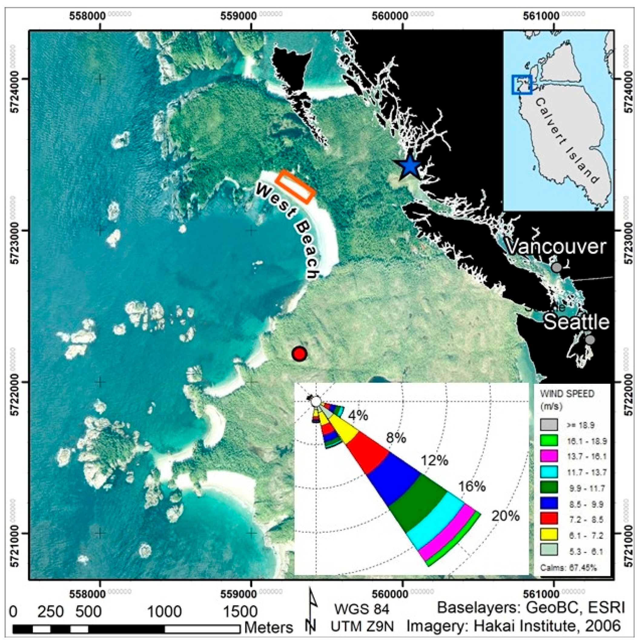
The study site is located on Calvert Island, on the central coast of British Columbia, Canada (Figure 5). The study was part of a collaborative research program on Coastal Sand Ecosystems in partnership with the Hakai Institute. Weather data from a nearby meteorological station for 2012 to 2016 shows prevailing winds from the SE (obliquely alongshore), a unimodal resultant drift potential (RDP), and a resultant drift direction of 317° derived using the Fryberger and Dean (1979) [32] model and following the approach of Miot da Silva and Hesp [33]. The experiment was conducted on West Beach, a 1 km wide embayed, shallow sloping (1.8° average intertidal slope), sandy beach bounded by rocky headlands with a SE aspect (Figure 1). The West Beach foredune on the north end of the beach is approximately 6.5 m tall and partially vegetated with stoss slope angles of 23° to 37° and a crestline orientation of SE-NW (128°|308°). The foredune toe was incised by a 1 to 2 m scarp formed by a storm on 10 March 2016. The beach is macro-tidal with a spring tide range of >4 m and has a low tide width of 250 m and an effective fetch in the resultant drift direction of >500 m. D50 of beach-dune sediments is 0.198 mm with a calculated transport threshold of 5.3 m s−1 [34]. The foredune is predominantly vegetated by Elymus mollis and fronted by accumulations of LWD.
2.2. Experimental Setup
The experiment was conducted during 11–25 April 2016. Four shore-normal transects were established that remained fixed, but only the results from two transects are discussed (Figure 6) because the other two transects yielded consistent (duplicative) results. Shore-normal transects were established following convention for aeolian studies on coastal beaches and in anticipation of localized topographic steering of the regional wind field leading to oblique onshore winds. Transect (T1) was located within the LWD matrix, and Transect 2 (T2) was the reference transect, which was cleared of LWD to 4 m on either side of the transect (Figure 5). Two instrument stations were situated on each transect, one on the flat upper beach and a second on the stoss slope of the foredune (Figure 7). The stoss slope stations at T1 and T2 were both positioned 3 m landward of the scarp. The upper beach stations were at 4.5 m seaward of the scarp along T1 but 7 m seaward of the scarp along T2 (the reference station). During the experiment, T1 had different upwind LWD coverage due to changes in the obliquity (156° average) of the incoming wind direction (Table 1), whereas the beach station at T2 was not sufficiently far outside of the LWD to not be influenced by this altered roughness effect.
Ultrasonic anemometers (3D Gill WindMaster) were used to sample wind velocity components (, horizontal; , spanwise; and , vertical). All instruments were horizontally-aligned with the axis oriented offshore at 218° and axis alongshore at 128° SE (relative to true north; Magnetic Declination of +17°47′ East). All flow directions are presented relative to the dune crestline (0° alongshore, 90° onshore) unless otherwise noted. Each instrument station consisted of two 3D sonics mounted on an aluminum frame at 0.5 m (inverted) and 1.5 m (upright) above the surface (Figure 8a,b). The 0.5 m height placed the anemometer just above the average LWD height (approximately 0.25 m, measured from terrestrial laser scans) so as avoid complex eddy shedding in the wake of individual pieces of LWD. Care was taken to clean the sensor nodes throughout the day and between runs to reduce moisture and dust contamination.
All electronic instruments were hard-wired to Hobo® EnergyPro Data Loggers (Onset Computer Corporation® part # H22-001) housed in weather-resistant cases adjacent to the transects. All data were sampled and recorded at 1 Hz. Standard data conversion routines were applied following manufacturers’ recommended guidelines.
2.3. Data Description and Analysis
The events examined in this study include a subset of eight 10-min runs from the 13 April and 15 April of 2016 (Figure 9). Runs were selected for analysis based on greatest sustained wind speeds, limited directional deviation, and presence of transport activity. Although the transport data are not described in this paper, the Wenglor activity records shown in Figure 9 were used solely in this paper to identify periods when transport was most active. All anemometer data were normalized by the data from T2B1.5 to portray relative spatial trends (normalizing equations are found in the respective figure descriptions). Missing data during runs 6–8 are due to sensor malfunctions.
Velocity data from the sonic anemometers were rotated to account for yaw and pitch alignments relative to the incident streamlines [4,35,36,37]. Yaw rotations used the following equations:
in which and are yaw adjusted values, alpha () is the time-averaged angle derived from U and V, which are the time-averaged velocity vectors for the sampling interval.
The yaw rotation transforms the horizontal coordinates toward a resultant speed such that the spanwise signal has zero mean. Pitch rotations used the following equations:
in which and are pitch and yaw adjusted values. Phi is the angle of the incoming streamline relative to the sensor plane (mounted horizontally) derived from , which is the mean horizontal velocity in the streamwise direction after yaw rotation, and is the time-averaged vertical velocity vector from the original time series for the sampling interval. Fluctuating components , , ) were calculated as follows:
in which , , are the time-averaged velocity vectors for the sampling interval derived from the yaw and pitch adjusted data.
Turbulent stresses and other flow parameters were then calculated from the rotated component time series. Reynolds kinematic normal stresses () were calculated as the variance of the velocity components , , ) using Equation (10) while the standard deviation was calculated as the square root of the variance (VAR) using Equation (11):
Turbulent Kinetic Energy (TKE) (m2·s−2) quantifies the total kinetic energy of the fluctuating flow, or how much the airflow deviates from its mean components, using Equation (12):
Kinematic Reynolds stress (RSk) is the time-averaged covariance of the streamwise and vertical fluctuating components, which characterizes the average vertical flux of streamwise momentum, using Equation (13):
The parameterization in Equation (13) assumes that there is relatively little fluctuation in the spanwise direction (e.g., as in a wind tunnel), but with natural flows across LWD, there can be significant spanwise wind energy. The horizontal kinematic Reynolds stress () captures the degree of correlation between the additional spanwise and vertical fluctuations using Equation (14) [3,35]:
Turbulence Intensity (in the streamwise direction) is characterized by the coefficient of variation (), which assesses the magnitude of wind speed fluctuations relative to the mean flow using Equation (15):
For the sake of simplicity, all future references to , , and , , in this paper should be considered as referring to the yaw and pitch adjusted values (with the subscripts dropped) unless specifically noted.
Fluctuating velocity components ( and ) were used to produce quadrant plots that show the stress geometry of turbulent flow in graphical form (Figure 10).
3. Results and Discussion
3.1. Flow Dynamics over LWD
Flow properties over the LWD are compared to conditions over the beach with no LWD using normalized quantities. All runs were averaged to establish a baseline from which to assess deviations from the mean (normalized) state. For example, differences in time between the various runs can be assessed relative to the overall mean for all runs, and similarly, the relative deviation of T1 away from T2 for all runs provides an indication of the influence of LWD on flow dynamics. A summary of observed flow properties averaged over the eight selected runs (Figure 9) is provided in Table 2 and a complete list of flow properties for individual 10-min runs is found in Appendix A. Average incoming wind speed at the reference station for all eight runs was 4.8 m s−1 while average incoming wind direction was 28°. Figure 11 is based on the data in Table 2 and portrays graphically the quantities at T1 (LWD) in terms of the percent difference from T2 (the reference site with no LWD). Percentages indicate a relative decrease (negative) or increase (positive) of flow quantities.
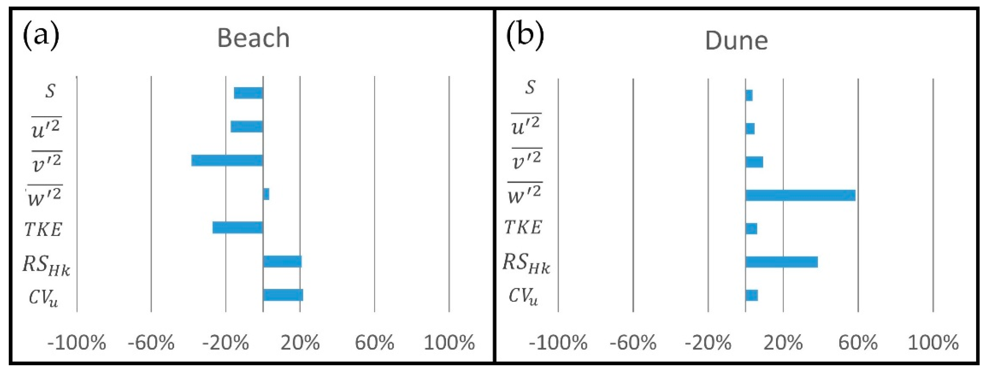
LWD fronting the foredune had a clear and measurable effect on flow over the upper beach and was highly effective at altering flow characteristics measured at both 1.5 and 0.5 m (Figure 11). Overall, there were consistent decreases in mean wind speed (S), spanwise normal stress (), turbulent kinetic energy (TKE) at T1 (with LWD) relative to T2 (without LWD). Similarly, there was a consistent increase in turbulence intensity () at T1. These differences in flow dynamics in the presence of LWD indicate that the enhanced roughness exerts additional drag on the flow field, extracting energy from the mean flow (i.e., decrease in S and TKE) and converting it to enhanced turbulent motion (i.e., increase in ). Also noteworthy is the near 60% increase in on the beach resulting from flow deflection up and over the LWD, despite the small magnitude of the vertical motions relative to the horizontal components.
The 50% reduction in at T1B0.5 can be attributed to two primary factors. First, the LWD-induced drag close to the sand surface reduces overall mean and fluctuating energy because the wind slows down within the LWD matrix (Table 2). Second, spanwise fluctuations are subdued because the individual logs act as physical barriers to lateral flow, and therefore the wind is directed up and over the LWD. In this way, spanwise fluctuating energy is transformed into vertical fluctuating energy. The strong increase in at T1B0.5 (Figure 12, bottom) supports this assertion.
The roughness drag induced by the LWD matrix created a strongly sheared flow zone between the sand surface and the flow layer above the LWD matrix. However, net remained nearly the same at T1 and T2 (Figure 11b). Wind speed and TKE were smaller at T1 by about 30%, indicating an extraction of mean energy from the flow (Figure 11b). The quadrant plots (Figure 12) show that the magnitude of occurrences at T1B0.5, remained relatively small compared to the magnitude of , despite a 60% increase in the absolute value of from T2 to T1. Even though the increase in is relatively small, it is visible on the T1B0.5 quadrant plot, which shows an orientation favoring a Q2:Q4 alignment. In contrast, is not affected as much as the other quantities at T1B0.5. The actual values are simply so small relative to that the contribution to from the increase in is minor and nearly balanced by the −13% decrease in . Net therefore remains nearly unchanged despite the increased drag and shear, and conversion of mean to turbulent energy.
LWD did not have the same effect on flow over the stoss slope of the dune. The majority of changes on the dune are within 10% of the reference values and are generally less pronounced than over the beach as documented in Figure 13 (thematically identical to Figure 11). Notable reductions in and are most likely the result of the presence of a 1.8 m tall scarp on T2, rather than the influence of LWD. The larger scarp on T2 generates greater vertical fluctuations (, Figure 14) and disrupts flow modulations (e.g., topographically forced flow compression, acceleration, and streamline curvature) that inhibit turbulent motions [14,25,40,41]. This influence makes attributing changes to flow properties on the dune to the presence of upwind LWD problematic, and should not be interpreted as absolute, but rather as a general characterization. Still, the minimal change to all other flow properties suggests that characteristic flow modulations that occur in the presence of large dunes are pronounced and dominate flow characteristics, regardless of the presence of LWD upwind of the dune.
The LWD had a more pronounced effect on the flow closer to the beach surface (at 0.5 m) than immediately above the LWD matrix (at 1.5 m). Figure 15 shows the deviation of the change between the T10.5 and T11.5 anemometers at the beach and dune stations relative to those on T2. A value of zero (negative; positive) indicates the change between the T10.5 and T11.5 anemometers was the same as (greater than; less than) the change between the T20.5 and T21.5 anemometers, even if the absolute values between transects varied. Reductions in S, , , and on the beach (shown in Figure 15a) indicate that the drag effect induced by LWD is stronger closer to the surface. The LWD was also effective at converting mean energy to streamwise turbulent energy at 0.5 m, based on the increase in . On the dune, all of the flow quantities increased, supporting the observation that flow adjustments at 0.5 m were dominated by the presence of the dune and not the upwind LWD.
3.2. Flow Steering over LWD
Flow direction on the reference transect at the beach station (T2B1.5 and T2B0.5) shows minimal deviation from the reference condition at T2B1.5 (Table 3). Flow across the dune profile along T2, however, was steered towards crest normal, in agreement with previous research on oblique flow over a stoss slope [13,41,42,43,44]. In contrast, flow direction on T1, with LWD, was altered to a much greater degree than along the reference transect with no LWD (Table 3). Results over T1 at both the beach and dune locations varied by run and day. Runs 1–4 (13 April), with mean wind angle of 14°, recorded mostly onshore steering, while runs 5–8 (15 April), with mean wind angle of 38° (0° alongshore, 90° onshore), recorded alongshore steering at the same locations. Therefore, the predominantly onshore flow was steered alongshore in a manner similar to deflection in the presence of a scarp [43], whereas the obliquely alongshore flow was steered towards the dune, similar to findings from other studies of flow over foredunes [8,41,45,46,47].
It is possible that LWD on the beach contributed to the observed flow steering patterns, however, the presence of a larger scarp and taller dune on T2 complicates any causal association. The LWD matrix as arranged during this study was fairly low in height (<0.5 m) with few stacked logs resulting in mostly shore-parallel or acute alignments (see Figure 6 and Figure 8a), thus providing a short, non-porous physical barrier that could steer flow alongshore. The drag-induced flow speed reduction over the LWD at 0.5 m could create a pressure differential between the faster flow observed on the stoss slope, thus steering alongshore flow toward the faster and lower pressure flow on the dune. However, T1B was placed 3.5 m closer to the dune crest than the reference station T2B, which was intentionally placed farther seaward to avoid effects of the taller scarp (+1 m) and dune (+2.5 m). As a result, the flow steering over the LWD cannot be conclusively linked to the presence of LWD since the effects of T1B being placed closer to the dune are unknown. Unfortunately, the incident flow angle for this study did not vary more than 30° and additional data from multiple and highly variable wind approach angles with similar landward dune characteristics is necessary to fully realize the effects of LWD matrices and LWD orientation on flow steering.
3.3. Implications of Flow over LWD for Beach-Dune System Morphodynamics
Analysis of turbulent flow properties over LWD on the beach and on the dune stoss slope provides the basis for a discussion of the potential implications for sand transport and dune morphodynamics. The overall effect of the LWD matrix was to reduce near-surface wind speed, Reynolds Normal Stress, and turbulent energy while simultaneously transferring energy from the mean flow field to the fluctuating components, as shown by increases in . The increased demonstrates that the LWD matrix facilitates a transfer of energy from the mean flow to the turbulent fluctuations. This cascade of energy toward enhanced turbulence might suggest an increased capacity to transport sediment, but values such as , which have been shown to have a stronger role in sediment transport [9,14,48,49,50,51], decreased over the LWD (Table 2). Similarly, the absolute reduction in streamwise fluctuations relative to the increase in vertical fluctuations results in remaining nearly static. Therefore the LWD matrix acts effectively as a pseudo-stagnation zone in front of the dune, which can serve as a sink for sediment deposition.
Changes to flow quantities downwind of the LWD indicate the potential for sediment transport on the stoss slope of the dune despite the flow alterations caused by LWD on the beach. The increase in and (Figure 15b) as well as Q2 and Q4 occurrences at T1D0.5 compared to T1D1.5 (Figure 14) confirm that turbulent structures are conveyed toward the bed. The Quadrant occurrences are consistent with the increase in as the Q2 and Q4 interactions contribute positively to Reynolds stress. Turbulent structures conveyed toward the bed are the result of topographic forcing (i.e., flow compression and streamline concavity) [52]. Thus, transport could still be active on the stoss slope of the foredune (e.g., [9]) downwind of the LWD.
3.4. Limitations
As LWD matrices are inherently diverse and complex, and since the data collected during this study span a relatively limited range of conditions, the conclusions are necessarily site and event specific. It is important to remember that this study monitored wind speeds over a fairly limited range, averaging 3.7 and 6.1 m s−1 gusting to 11.0 and 12.2 m s−1 which produced highly intermittent and spatially variable sand transport that may not be representative of conditions during sustained winds with greater energy. Further research is needed to fully capture the range of conditions that may prove the importance of LWD in modifying wind and transport conditions across beach-dune systems. In particular, variations in LWD matrix height, depth, density, and stage of infilling should be measured to ascertain their effect on flow alterations.
Comparing flow over LWD to flow over a reference transect with no LWD is desirable, but difficult to achieve in the field. Variations in dune height and topography, presence of a scarp (and scarp height), vegetation density and variability, and the ability to clear the LWD make comparing different locations on the beach problematic. Indeed, this study refers to T2 as the reference transect, yet the highly alongshore nature of flow resulted in the T2 dune station being influenced slightly by LWD, as evidenced by the coverage density in Table 1. Future experiments would likely benefit from locating additional instrumentation within, up-, and down-wind of the matrix while referencing changes in flow conditions relative to fully developed boundary layer flow over the beach, thus eliminating impacts from variable morphology and the need for a transect with no LWD.
4. Conclusions
The effects of LWD on turbulent airflow over an embayed sandy beach-dune system were investigated. Sonic 3D anemometry was used to quantify flow and turbulence quantities over and through a LWD matrix (approximately 12 m wide and <0.5 m in height) fronting the foredune during highly oblique alongshore flow and limited wind speeds. The main findings are:
- LWD acts as a highly effective flow modifier over the beach by inducing roughness drag that serves to deflect the incoming flow upward and away from the surface. The absolute magnitude of near-surface mean wind speed, turbulent kinetic energy, and Reynolds stress are reduced in the presence of a LWD matrix. In addition, there is a transfer of energy from the mean flow field to the turbulent fluctuations, such that the overall turbulence intensity increases along with a slight shift in the quadrant geometry toward Q2/Q4 event activity. These flow modifications would seem to favor sediment transport potential, but not so in light of the overall reductions in the mean energy of the flow field. The effect of the LWD matrix on flow considered in this paper does not include the localized flow patterns around individual pieces of LWD nor the substantial physical barrier they present to saltating grains.
- Shore-parallel aligned LWD has the potential to cause alongshore flow steering of obliquely onshore winds, although this depends on incoming flow angle. An alongshore flow steering effect of highly oblique incident winds could enhance the decoupling effect of beach and dune sediment transport pathways described by Bauer et al. [42] minimizing landward transport [53].
- Downwind of the LWD, on the stoss slope of the dune, there is evidence of flow compression and streamline concavity that conveys turbulent flow structures toward the bed. The presence of these flow patterns suggests that flow downwind of a LWD matrix responds characteristically to topographic forcing as would be expected in the absence of LWD, thus providing the potential for sediment transport on the stoss slope of the dune.
Author Contributions
Michael J. Grilliot, Ian J. Walker, and Bernard O. Bauer conceived, designed, and performed the experiments; Michael J. Grilliot analyzed the data with guidance from Ian J. Walker and Bernard O. Bauer; Ian J. Walker and Bernard O. Bauer contributed equipment and analysis tools; Michael J. Grilliot wrote the first draft of the paper with thematic guidance and editorial assistance from Ian J. Walker and Bernard O. Bauer.
Acknowledgments
This research was supported financially and logistically by partners at the Hakai Institute and Tula Foundation, notably Eric Peterson and Christina Munck. This project was also funded by a Hakai Ph.D. Fellowship to Michael J. Grilliot, NSERC Discovery and CFI grants to Ian J. Walker. Field assistance was provided by staff from the Hakai Institute and many graduate students in the CEDD laboratory at UVic, in particular, Derek Heathfield (Hakai), Alana Rader (UVic), and Felipe Gomez (UVic). The authors recognize that this study took place on the traditional territory of the Heiltsuk and Wuikinuxv First Nations, and are grateful for the opportunity. The authors thank issue guest editor Eric J. R. Parteli and two anonymous reviewers for their constructive comments and suggestions that improved the quality of the manuscript.
Conflicts of Interest
The authors declare no conflict of interest. The founding sponsors had no role in the design of the study; in the collection, analyses, or interpretation of data; in the writing of the manuscript, and in the decision to publish the results.
Appendix A
Summary of observed flow properties for each 10 min run including surface slope angle and incident flow angle (degrees), resultant 3D wind speed (S, m s−1), flow streamline angles (degrees), Normal Reynolds stresses (, m2 s−2), total kinetic energy (TKE, m2 s−2), Horizontal kinematic Reynolds stress (, m2 s−2), and coefficient of variation (CVu). Flow angle is relative to true north. Streamline angles and surface slope angles are relative to horizontal (0°).

| T1 (LWD) | T2 (No LWD) | |||||||
|---|---|---|---|---|---|---|---|---|
| Beach Lower (0.5 m) | Beach Upper (1.5 m) | Stoss Lower (0.5 m) | Stoss Upper (1.5 m) | Beach Lower (0.5 m) | Beach Upper (1.5 m) | Stoss Lower (0.5 m) | Stoss Upper (1.5 m) | |
| surface slope angle (o) | −4 | −4 | −23 | −23 | −4 | −4 | −37 | −37 |
| 13 April 2016 | ||||||||
| Run 1 (13:35:20–13:45:19) | ||||||||
| Flow angle (o) | 151 | 153 | 145 | 148 | 152 | 153 | 159 | 155 |
| S | 2.4 | 3.2 | 2.3 | 2.9 | 3.5 | 3.8 | 2.7 | 3.2 |
| Streamline angle (o) | −3 | −3 | −8 | −10 | 0 | −2 | −16 | −16 |
| 2.03 | 2.61 | 1.11 | 1.61 | 2.01 | 2.15 | 1.41 | 1.72 | |
| 0.63 | 1.24 | 0.89 | 1.15 | 1.21 | 1.38 | 1.17 | 1.52 | |
| 0.08 | 0.15 | 0.18 | 0.24 | 0.04 | 0.10 | 0.27 | 0.40 | |
| TKE | 1.37 | 2.00 | 1.09 | 1.51 | 1.63 | 1.82 | 1.43 | 1.82 |
| 0.11 | 0.08 | 1.61 | 0.31 | 0.09 | 0.10 | 0.47 | 0.57 | |
| CVu | 0.67 | 0.57 | 0.53 | 0.50 | 0.43 | 0.41 | 0.52 | 0.47 |
| Run 2 (13:56:40–14:06:39) | ||||||||
| Flow angle (o) | 161 | 161 | 162 | 159 | 151 | 151 | 155 | 151 |
| S | 1.8 | 2.6 | 2.0 | 2.4 | 3.1 | 3.3 | 2.2 | 2.6 |
| Streamline angle (o) | −7 | −3 | −12 | −10 | 0 | −2 | −15 | −14 |
| 1.77 | 2.59 | 1.48 | 1.87 | 2.17 | 2.27 | 1.51 | 1.71 | |
| 0.70 | 1.20 | 1.19 | 1.20 | 1.66 | 1.55 | 1.12 | 1.27 | |
| 0.09 | 0.21 | 0.16 | 0.29 | 0.06 | 0.14 | 0.26 | 0.37 | |
| TKE | 1.28 | 2.00 | 1.42 | 1.68 | 1.95 | 1.98 | 1.44 | 1.68 |
| 0.19 | 0.04 | 1.87 | 0.25 | 0.16 | 0.13 | 0.43 | 0.47 | |
| CVu | 0.96 | 0.77 | 0.87 | 0.72 | 0.54 | 0.51 | 0.68 | 0.61 |
| Run 3 (14:43:50–14:53:49) | ||||||||
| Flow angle (o) | 155 | 158 | 152 | 150 | 144 | 144 | 155 | 151 |
| S | 2.6 | 3.5 | 2.6 | 3.2 | 3.9 | 4.2 | 3.0 | 3.5 |
| Streamline angle (o) | −6 | −3 | −10 | −8 | 0 | −1 | −15 | −13 |
| 2.37 | 3.86 | 2.27 | 3.39 | 3.46 | 3.76 | 2.30 | 3.02 | |
| 1.15 | 1.97 | 1.91 | 1.99 | 2.66 | 2.82 | 1.67 | 1.90 | |
| 0.13 | 0.23 | 0.27 | 0.49 | 0.07 | 0.20 | 0.39 | 0.70 | |
| TKE | 1.83 | 3.04 | 2.23 | 2.94 | 3.10 | 3.39 | 2.18 | 2.81 |
| 0.24 | 0.14 | 3.39 | 0.53 | 0.23 | 0.34 | 0.66 | 0.81 | |
| CVu | 0.73 | 0.66 | 0.77 | 0.72 | 0.54 | 0.51 | 0.60 | 0.56 |
| Run 4 (15:05:50–15:15:49) | ||||||||
| Flow angle (o) | 157 | 159 | 153 | 153 | 141 | 143 | 150 | 146 |
| S | 2.1 | 3.0 | 2.2 | 2.7 | 3.4 | 3.7 | 2.6 | 3.1 |
| Streamline angle (o) | −9 | −3 | −11 | −7 | 0 | −2 | −12 | −12 |
| 1.88 | 2.82 | 1.49 | 2.06 | 2.91 | 3.33 | 2.09 | 2.46 | |
| 0.72 | 1.13 | 1.21 | 1.28 | 1.46 | 1.46 | 1.00 | 1.19 | |
| 0.10 | 0.19 | 0.23 | 0.34 | 0.04 | 0.14 | 0.30 | 0.45 | |
| TKE | 1.35 | 2.07 | 1.47 | 1.84 | 2.21 | 2.47 | 1.70 | 2.05 |
| 0.27 | 0.06 | 2.06 | 0.30 | 0.12 | 0.15 | 0.45 | 0.48 | |
| CVu | 0.75 | 0.62 | 0.71 | 0.61 | 0.54 | 0.53 | 0.62 | 0.57 |
| 15 April 2016 | ||||||||
| Run 5 (11:22:00–11:31:59) | ||||||||
| Flow angle (o) | 152 | 161 | 157 | 160 | 170 | 172 | 174 | 172 |
| S | 3.3 | 4.7 | 3.5 | 4.4 | 4.6 | 5.2 | 3.6 | 4.3 |
| Streamline angle (o) | −1 | −5 | −8 | −11 | −1 | −4 | −21 | −20 |
| 1.19 | 1.42 | 1.11 | 1.39 | 1.05 | 1.29 | 0.92 | 1.14 | |
| 1.02 | 2.26 | 1.81 | 2.30 | 2.27 | 2.63 | 2.17 | 2.63 | |
| 0.11 | 0.14 | 0.23 | 0.30 | 0.03 | 0.09 | 0.32 | 0.42 | |
| TKE | 1.16 | 1.91 | 1.57 | 2.00 | 1.67 | 2.01 | 1.70 | 2.10 |
| 0.07 | 0.16 | 0.47 | 0.59 | 0.13 | 0.24 | 0.71 | 0.70 | |
| CVu | 0.35 | 0.27 | 0.32 | 0.29 | 0.23 | 0.23 | 0.30 | 0.27 |
| Run 6 (11:43:54–11:52:53) | ||||||||
| Flow angle (o) | 147 | 155 | 148 | 157 | 160 | 162 | 161 | |
| S | 4.0 | 5.5 | 4.4 | 5.4 | 6.1 | 4.6 | 5.4 | |
| Streamline angle (o) | −1 | −5 | −6 | −1 | −3 | −17 | −16 | |
| 1.66 | 2.27 | 1.86 | 1.71 | 2.13 | 1.74 | 1.98 | ||
| 1.06 | 2.69 | 1.81 | 2.43 | 2.80 | 2.43 | 3.08 | ||
| 0.11 | 0.15 | 0.28 | 0.03 | 0.09 | 0.41 | 0.49 | ||
| TKE | 1.42 | 2.56 | 1.98 | 2.09 | 2.51 | 2.29 | 2.78 | |
| 0.14 | 0.27 | 0.65 | 0.18 | 0.24 | 0.96 | 0.97 | ||
| CVu | 0.34 | 0.29 | 0.33 | 0.25 | 0.25 | 0.31 | 0.28 | |
| Run 7 (12:09:30–12:19:29) | ||||||||
| Flow angle (o) | 149 | 158 | 155 | 167 | 169 | 172 | 171 | |
| S | 3.6 | 5.2 | 4.0 | 5.7 | 6.3 | 4.4 | 5.2 | |
| Streamline angle (o) | −1 | −5 | −8 | −1 | −4 | −20 | −19 | |
| 1.40 | 1.84 | 1.57 | 1.63 | 1.95 | 1.33 | 1.54 | ||
| 1.36 | 3.45 | 2.48 | 3.80 | 4.49 | 3.48 | 4.26 | ||
| 0.13 | 0.17 | 0.29 | 0.04 | 0.09 | 0.44 | 0.56 | ||
| TKE | 1.44 | 2.73 | 2.18 | 2.74 | 3.27 | 2.63 | 3.18 | |
| 0.12 | 0.29 | 0.73 | 0.24 | 0.35 | 1.06 | 1.22 | ||
| CVu | 0.35 | 0.28 | 0.34 | 0.24 | 0.23 | 0.29 | 0.26 | |
| Run 8 (13:31:00–13:40:59) | ||||||||
| Flow angle (o) | 144 | 152 | 144 | 152 | 154 | 155 | 155 | |
| S | 4.1 | 5.8 | 4.2 | 5.6 | 6.2 | 4.9 | 5.7 | |
| Streamline angle (o) | −1 | −5 | −6 | 0 | −3 | −15 | −14 | |
| 1.46 | 2.22 | 1.78 | 2.24 | 2.78 | 2.23 | 2.71 | ||
| 1.78 | 4.09 | 2.17 | 2.19 | 2.59 | 2.34 | 2.73 | ||
| 0.14 | 0.23 | 0.36 | 0.03 | 0.09 | 0.48 | 0.58 | ||
| TKE | 1.70 | 3.28 | 2.16 | 2.24 | 2.73 | 2.53 | 3.02 | |
| 0.15 | 0.36 | 0.71 | 0.14 | 0.20 | 1.05 | 1.15 | ||
| CVu | 0.32 | 0.27 | 0.34 | 0.28 | 0.28 | 0.33 | 0.30 | |
References
- Gillies, J.A.; Nield, J.M.; Nickling, W.G. Wind speed and sediment transport recovery in the lee of a vegetated and denuded nebkha within a nebkha dune field. Aeolian Res. 2014, 12, 135–141. [Google Scholar] [CrossRef]
- Hesp, P.A. Foredunes and blowouts: Initiation, geomorphology and dynamics. Geomorphology 2002, 48, 245–268. [Google Scholar] [CrossRef]
- Mayaud, J.R.; Wiggs, G.F.S.; Bailey, R.M. Characterizing turbulent wind flow around dryland vegetation. Earth Surf. Process. Landf. 2016, 1436, 1421–1436. [Google Scholar] [CrossRef]
- Mayaud, J.R.; Wiggs, G.F.S.; Bailey, R.M. Dynamics of skimming flow in the wake of a vegetation patch. Aeolian Res. 2016, 22, 141–151. [Google Scholar] [CrossRef]
- Wolfe, S.A.; Nickling, W.G. The protective role of sparse vegetation in wind erosion. Prog. Phys. Geogr. 1993, 17, 50–68. [Google Scholar] [CrossRef]
- Arens, S.M. Patterns of sand transport on vegetated foredunes. Geomorphology 1996, 17, 339–350. [Google Scholar] [CrossRef]
- Arens, S.M.; Slings, Q.; de Vries, C.N. Mobility of a remobilised parabolic dune in Kennemerland, The Netherlands. Geomorphology 2004, 59, 175–188. [Google Scholar] [CrossRef]
- Arens, S.M.; Van Kaam-Peters, H.M.E.; Van Boxel, J.H. Air flow over foredunes and implications for sand transport. Earth Surf. Process. Landf. 1995, 20, 315–332. [Google Scholar] [CrossRef]
- Chapman, C.; Walker, I.J.; Hesp, P.A.; Bauer, B.O.; Davidson-Arnott, R.G.D.; Ollerhead, J. Reynolds stress and sand transport over a foredune. Earth Surf. Process. Landf. 2013, 38, 1735–1747. [Google Scholar] [CrossRef]
- Davidson-Arnott, R.G.D.; Bauer, B.O.; Walker, I.J.; Hesp, P.A.; Ollerhead, J.; Chapman, C. High-frequency sediment transport responses on a vegetated foredune. Earth Surf. Process. Landf. 2012, 37, 1227–1241. [Google Scholar] [CrossRef]
- Hesp, P.A.; Smyth, T.A.G.G. Nebkha flow dynamics and shadow dune formation. Geomorphology 2017, 282, 27–38. [Google Scholar] [CrossRef]
- Keijsers, J.G.S.; De Groot, A.V.; Riksen, M.J.P.M. Vegetation and sedimentation on coastal foredunes. Geomorphology 2015, 228, 723–734. [Google Scholar] [CrossRef]
- Walker, I.J.; Barrie, J.V. Geomorphology and sea-level rise on one of Canada’s most sensitive coasts: Northeast Graham Island, British Columbia. J. Coast. Res. 2006, 39, 220–226. [Google Scholar]
- Bauer, B.O. Fundamentals of Aeolian Sediment Transport: Boundary-Layer Processes. In Treatise on Geomorphology, 1st ed.; Shroder, J.F., Lancaster, N., Sherman, D.J., Baas, A.C.W., Eds.; Elsevier Ltd.: San Diego, CA, USA, 2013; Volume 11.2, pp. 7–22. [Google Scholar]
- McKenna Neuman, C.; Bédard, O. A wind tunnel study of flow structure adjustment on deformable sand beds containing a surface-mounted obstacle. J. Geophys. Res. Earth Surf. 2015, 120, 1824–1840. [Google Scholar] [CrossRef]
- Sutton, S.L.F.; McKenna Neuman, C. Sediment entrainment to the lee of roughness elements: Effects of vortical structures. J. Geophys. Res. Earth Surf. 2008, 113, 1–7. [Google Scholar] [CrossRef]
- Gillies, J.A.; Green, H.; McCarley-Holder, G.; Grimm, S.; Howard, C.; Barbieri, N.; Ono, D.; Schade, T. Using solid element roughness to control sand movement: Keeler Dunes, Keeler, California. Aeolian Res. 2015, 18, 35–46. [Google Scholar] [CrossRef]
- Gillies, J.A.; Lancaster, N. Large roughness element effects on sand transport, Oceano Dunes, California. Earth Surf. Process. Landf. 2013, 38, 785–792. [Google Scholar] [CrossRef]
- Gillies, J.A.; Nickling, W.G.; King, J. Aeolian sediment transport through large patches of roughness in the atmospheric inertial sublayer. J. Geophys. Res. 2006, 111, F02006. [Google Scholar] [CrossRef]
- Eamer, J.B.R.; Walker, I.J. Quantifying sand storage capacity of large woody debris on beaches using LiDAR. Geomorphology 2010, 118, 33–47. [Google Scholar] [CrossRef]
- Baddock, M.C.; Wiggs, G.F.S.; Livingstone, I. A field study of mean and turbulent flow characteristics upwind, over and downwind of barchan dunes. Earth Surf. Process. Landf. 2011, 36, 1435–1448. [Google Scholar] [CrossRef]
- Lee, B.E.; Soliman, B.F. An Investigation of the Forces on Three Dimensional Bluff Bodies in Rough Wall Turbulent Boundary Layers. J. Fluids Eng. 1977, 99, 503–510. [Google Scholar] [CrossRef]
- Raupach, M.R. Drag and drag partition on rough surfaces. Bound.-Layer Meteorol. 1992, 60, 375–395. [Google Scholar] [CrossRef]
- Raupach, M.R.; Gillette, D.A.; Leys, J.F. The effect of roughness elements on wind erosion threshold. J. Geophys. Res. 1993, 98, 3023–3029. [Google Scholar] [CrossRef]
- Wiggs, G.F.S.; Livingstone, I.; Warren, A. The role of streamline curvature in sand dune dynamics: Evidence from field and wind tunnel measurements. Geomorphology 1996, 17, 29–46. [Google Scholar] [CrossRef]
- Iversen, J.D.; Wang, W.-P.; Rasmussen, K.R.; Mikkelsen, H.E.; Hasiuk, J.F.; Leach, R.N. The effect of a roughness element on local saltation transport. J. Wind Eng. Ind. Aerodyn. 1990, 36, 845–854. [Google Scholar] [CrossRef]
- Lancaster, N. Geomorphology of Desert Dunes, 1st ed.; Routledge: New York, NY, USA, 1995. [Google Scholar]
- Leenders, J.K.; van Boxel, J.H.; Sterk, G. The effect of single vegetation elements on wind speed and sediment transport in the Sahelian zone of Burkina Faso. Earth Surf. Process. Landf. 2007, 32, 1454–1474. [Google Scholar] [CrossRef]
- Pattenden, R.J.; Turnock, S.R.; Zhang, X. Measurements of the flow over a low-aspect-ratio cylinder mounted on a ground plane. Exp. Fluids 2005, 39, 10–21. [Google Scholar] [CrossRef]
- Gillies, J.A.; Nickling, W.G.; King, J. Shear stress partitioning in large patches of roughness in the atmospheric inertial sublayer. Bound.-Layer Meteorol. 2007, 122, 367–396. [Google Scholar] [CrossRef]
- Lancaster, N.; Baas, A. Influence of vegetation cover on sand transport by wind: Field studies at Owens Lake, California. Earth Surf. Process. Landf. 1998, 23, 69–82. [Google Scholar] [CrossRef]
- Fryberger, S.G.; Dean, G. Dune Forms and Wind Regime. In A Study Glob. Sand Seas; McKee, E.D., Ed.; USGS Professional Paper 1052; US Geological Survey and United States National Aeronautics and Space Administration: Washington, DC, USA, 1979; pp. 137–170. [Google Scholar]
- Miot da Silva, G.; Hesp, P. Coastline orientation, aeolian sediment transport and foredune and dunefield dynamics of Moçambique Beach, Southern Brazil. Geomorphology 2010, 120, 258–278. [Google Scholar] [CrossRef]
- Eamer, J.B.R. Reconstruction of the Late Pleistocene and Holocene Geomorphology of Northwest Calvert Island, British Columbia; University of Victoria: Victoria, BC, Canada, 2017; Available online: http://hdl.handle.net/1828/7944 (accessed on 12 June 2017).
- Lee, Z.S.; Baas, A.C.W. Streamline correction for the analysis of boundary layer turbulence. Geomorphology 2012, 171–172, 69–82. [Google Scholar] [CrossRef]
- Van Boxel, J.H.; Sterk, G.; Arens, S.M. Sonic anemometers in aeolian sediment transport research. Geomorphology 2004, 59, 131–147. [Google Scholar] [CrossRef]
- Walker, I.J. Physical and logistical considerations of using ultrasonic anemometers in aeolian sediment transport research. Geomorphology 2005, 68, 57–76. [Google Scholar] [CrossRef]
- Lu, S.S.; Willmarth, W.W. Measurements of the structure of the Reynolds stress in a turbulent boundary layer. J. Fluid Mech. 1973, 60, 481–511. [Google Scholar] [CrossRef]
- Sarkar, S.; Dey, S. Double-averaging turbulence characteristics in flows over a gravel bed. J. Hydraul. Res. 2010, 48, 801–809. [Google Scholar] [CrossRef]
- Frank, A.J.; Kocurek, G. Airflow up the stoss slope of sand dunes: Limitations of current understanding. Geomorphology 1996, 17, 47–54. [Google Scholar] [CrossRef]
- Walker, I.J.; Hesp, P.A.; Davidson-Arnott, R.G.D.; Bauer, B.O.; Namikas, S.L.; Ollerhead, J. Responses of three-dimensional flow to variations in the angle of incident wind and profile form of dunes: Greenwich Dunes, Prince Edward Island, Canada. Geomorphology 2009, 105, 127–138. [Google Scholar] [CrossRef]
- Bauer, B.O.; Davidson-Arnott, R.G.D.; Walker, I.J.; Hesp, P.A.; Ollerhead, J. Wind direction and complex sediment transport response across a beach-dune system. Earth Surf. Process. Landf. 2012, 37, 1661–1677. [Google Scholar] [CrossRef]
- Hesp, P.A.; Smyth, T.A.G.; Nielsen, P.; Walker, I.J.; Bauer, B.O.; Davidson-Arnott, R. Flow deflection over a foredune. Geomorphology 2015, 230, 64–74. [Google Scholar] [CrossRef]
- Walker, I.J.; Davidson-Arnott, R.G.D.; Bauer, B.O.; Hesp, P.A.; Delgado-Fernandez, I.; Ollerhead, J.; Smyth, T.A.G. Scale-dependent perspectives on the geomorphology and evolution of beach-dune systems. Earth-Sci. Rev. 2017. [Google Scholar] [CrossRef]
- Hesp, P.A.; Davidson-Arnott, R.; Walker, I.J.; Ollerhead, J. Flow dynamics over a foredune at Prince Edward Island, Canada. Geomorphology 2005, 65, 71–84. [Google Scholar] [CrossRef]
- Svasek, J.N.; Terwindt, J.H.J. Measurements of sand transport by wind on a natural beach. Sedimentology 1974, 21, 311–322. [Google Scholar] [CrossRef]
- Walker, I.J.; Hesp, P.A.; Davidson-Arnott, R.G.D.; Ollerhead, J. Topographic Steering of Alongshore Airflow over a Vegetated Foredune: Greenwich Dunes, Prince Edward Island, Canada. J. Coast. Res. 2006, 225, 1278–1291. [Google Scholar] [CrossRef]
- Bauer, B.O.; Walker, I.J.; Baas, A.C.W.; Jackson, D.W.T.; McKenna-Neuman, C.; Wiggs, G.F.S.; Hesp, P.A. Critical Reflections on the Coherent Flow Structures Paradigm in Aeolian Geomorphology. In Coherent Flow Structures Earth’s Surface; Venditti, J.G., Best, J.L., Church, M., Hardy, R.J., Eds.; John Wiley & Sons Ltd.: Chichester, UK, 2013; pp. 111–134. [Google Scholar] [CrossRef]
- Bauer, B.O.; Yi, J.; Namikas, S.L.; Sherman, D.J. Event detection and conditional averaging in unsteady aeolian systems. J. Arid Environ. 1998, 39, 345–375. [Google Scholar] [CrossRef]
- Sterk, G.; Jacobs, A.F.G.; van Boxel, J.H. The Effect of Turbulent Flow Structures on Saltation Sand Transport in the Atmospheric Boundary Layer. Earth Surf. Processes Landf. 1998, 887, 877–887. [Google Scholar] [CrossRef]
- Weaver, C.M.; Wiggs, G.F.S. Field measurements of mean and turbulent airflow over a barchan sand dune. Geomorphology 2011, 128, 32–41. [Google Scholar] [CrossRef]
- Chapman, C.A.; Walker, I.J.; Hesp, P.A.; Bauer, B.O.; Davidson-Arnott, R.G.D. Turbulent Reynolds stress and quadrant event activity in wind flow over a coastal foredune. Geomorphology 2012, 151–152, 1–12. [Google Scholar] [CrossRef]
- Ollerhead, J.; Davidson-Arnott, R.; Walker, I.J.; Mathew, S. Annual to decadal morphodynamics of the foredune system at Greenwich Dunes, Prince Edward Island, Canada. Earth Surf. Process. Landf. 2013, 38, 284–298. [Google Scholar] [CrossRef]
Figure 1.
(Left) Conceptualization of coherent flow structures surrounding a wall-mounted cylinder (Reproduced from McKenna Neuman and Bédard [15] p. 1827, originally from Pattenden et al. [29]). Copyright 2005, with permission from Springer Nature. (Right) Resulting morphology after a transporting event with height scale in mm (Reproduced from McKenna Neuman and Bédard [15] p. 1829). Copyright 2015, with permission from John Wiley and Sons.

Figure 2.
Flow regimes and associated theoretical wake development, shown in schematic plan and side view. Shaded areas are wake regions. The effect of different flow regimes on average (aerodynamic roughness) and (displacement height) per plant unit is shown. (Modified and reproduced from Mayaud et al. [4], p. 142 under the Creative Commons attribution license).

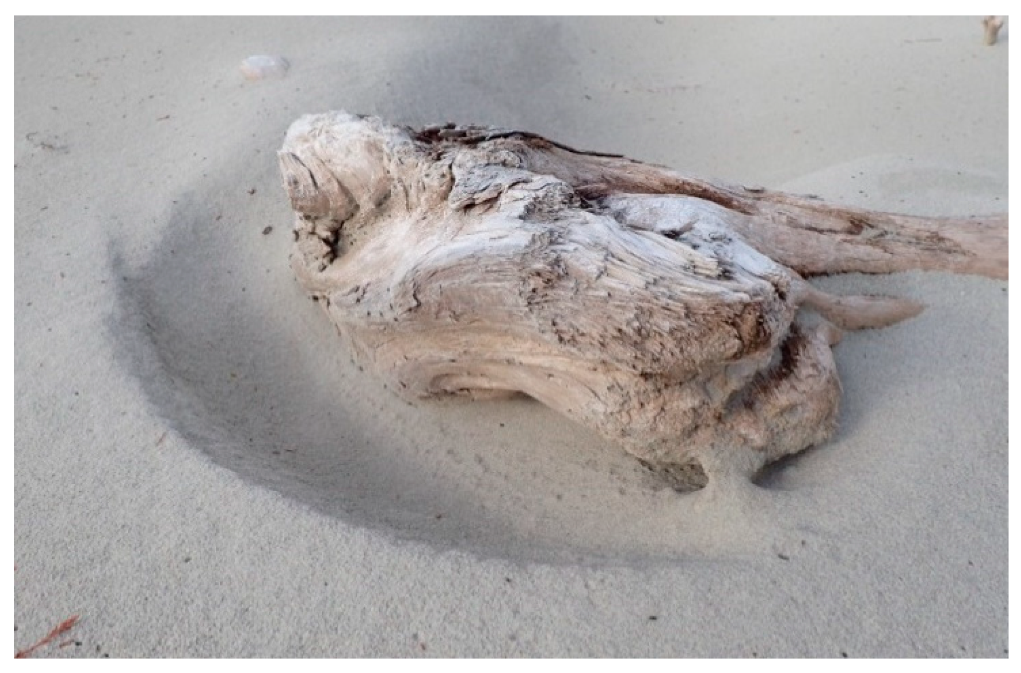
Figure 3.
Typical scour pattern due to horseshoe vortex around a piece of isolated LWD. Deflation hole is approximately 2 m in diameter. (photo credit: M. Grilliot).
Figure 3.
Typical scour pattern due to horseshoe vortex around a piece of isolated LWD. Deflation hole is approximately 2 m in diameter. (photo credit: M. Grilliot).

Figure 4.
Photos of LWD deposits commonly found on beaches around the world. Photo (a) shows a partially buried log with up- and down-wind sand ramps: Stewart Island, New Zealand; (b) shows a dense matrix of logs with appreciable amounts of aeolian deposition common on open coasts in British Columbia, Canada; (c) shows a matrix of LWD with near complete aeolian infilling in front an established foredune that was scarped by as much as 1.5 m one year before the photo was taken. Photo credits: (a) B. Bauer; (b) and (c) I. Walker.

Figure 5.
Location of the study area (orange rectangle) on West Beach, Calvert Island, British Columbia, Canada. Black overlay on the right shows the location of Calvert Island (blue star) in British Columbia. The upper-right inset shows the location of orthophoto detail (blue square). The red dot shows the location of the weather station used for the wind rose and drift rose (Figure 6) calculations.

Figure 6.
Aerial photo showing the location of transects 1 and 2 (T1, T2) as black lines and associated LWD coverage. LWD coverage is defined as the amount of plan-view surface area covered by LWD, extending 1 m on either side of the transect and 20 m seaward from the dune station. The arrow next to the reference station (i.e., not under the influence of LWD) indicates the average incoming wind direction at 1.5 m.

Figure 7.
Diagram of instrument locations along shore-normal transects T1 and T2. 3D sonic anemometer stations are labeled by transect number (T#) and beach (B) and dune (D) locations. Individual anemometers are referenced by downward-pointing triangles (0.5 m) and upward-pointing triangles (1.5 m). Anemometers are henceforth referred to via these designations and heights in subscript, e.g., the Transect 1 anemometer on the beach at 0.5 m is referred to as “T1B0.5”.

Figure 8.
Deployment of 3D anemometer flow measurement stations on T1 in the LWD on the beach (a) and dune (b), approximately 7.5 m apart. The upper anemometer is set at 1.5 m and the lower at 0.5 m.
Figure 8.
Deployment of 3D anemometer flow measurement stations on T1 in the LWD on the beach (a) and dune (b), approximately 7.5 m apart. The upper anemometer is set at 1.5 m and the lower at 0.5 m.

Figure 9.
Time series of incident wind speed (upper solid grey line with black 60 s running mean, upper left axis, m s−1), direction (middle dashed grey line with black 60 s running mean, right axis, degrees), and saltation intensity (bottom grey bars, bottom left axis, counts s−1) on 13 April (top graph) and 15 April (bottom graph). Wind speed and direction are from T2B1.5m and Saltation Intensity is from W1 (Figure 7). Runs are indicated on the top of each graph. The Wenglor (model YH08PCT8) laser particle counter (80 mm path length, 0.6 mm beam width, laser sampling beam was placed 0.031 m above the surface, located 5 m seaward from the LWD on T1, and aligned toward the incoming transport direction of 150°) was used to measure saltation intensity (counts −1).

Figure 10.
Quadrant plot with ± and ± axes. Quadrant 1 (Q1) is associated with outward interactions ( > 0, > 0), quadrant 2 (Q2) with ejections ( < 0, > 0), quadrant 3 (Q3) with inward interactions ( < 0, < 0), and quadrant 4 (Q4) with sweeps ( > 0, < 0).
Figure 10.
Quadrant plot with ± and ± axes. Quadrant 1 (Q1) is associated with outward interactions ( > 0, > 0), quadrant 2 (Q2) with ejections ( < 0, > 0), quadrant 3 (Q3) with inward interactions ( < 0, < 0), and quadrant 4 (Q4) with sweeps ( > 0, < 0).

Figure 11.
Percent difference in normalized flow quantities over the beach (calculated as: (T1 − T2)/T2B1.5) between similar anemometer locations on T1 (LWD) and T2 (no LWD) over all runs and flow quantities: resultant 3D wind speed (, m s−1), normal kinematic Reynolds stresses (, m2 s−2), turbulent kinetic energy (, m2 s−2), horizontal kinematic Reynolds stress (, m2 s−2), and the coefficient of variation ( ). (a) Beach 1.5 m; (b) Beach 0.5 m.

Figure 12.
Beach (T1B and T2B) Quadrant plots (1 Hz) for all runs (80 min, n = 4800). Each plot includes data from all eight runs to better visualize the gross distribution of components in the quadrant plots. However, only those fluctuations deemed to be significant (>1 standard deviation) are shown in the plots (total number in each quadrant is indicated by the values in the corners). The top right-hand corner also displays the mean incident flow angle (0° is alongshore, 90° is onshore), and wind speed (S) for all eight runs.

Figure 13.
Percent difference in normalized flow quantities over the stoss slope of the foredune (calculated as: (T1 − T2)/T2B1.5) between similar anemometer locations on T1 (LWD) and T2 (no LWD) over all runs and flow quantities: resultant 3D wind speed (, m s−1), normal kinematic Reynolds stresses (, m2 s−2), turbulent kinetic energy (, m2 s−2), horizontal kinematic Reynolds stress (, m2 s−2), and the coefficient of variation ( ). Top: Dune-1.5 m (excludes incomplete datasets from runs 6–8), Bottom: Dune-0.5 m.

Figure 14.
Dune (T1D and T2D) Quadrant plots (1 Hz) for all runs (80 min, n = 4800). For each quadrant, values for significant activity (>1 standard deviation) are shown in the corner. The top right-hand corner also displays the incident flow angle (0° is alongshore, 90° is onshore), and wind speed (S).

Figure 15.
Average normalized difference in flow quantities (calculated as: {(((T10.5 − T11.5) − (T20.5 − T21.5))/T2B1.5)} at height (0.5 m and 1.5 m) between T1 and T2 at the beach (a) and dune (b) using the same flow quantities as in Figure 11. Data were normalized to the 1.5 m beach anemometer on T2 (T2B1.5) for each run. The dune values (b) exclude incomplete datasets from runs 6–8.

Table 1.
Upwind LWD cover densities (%) based on average incoming wind direction of 28° (relative to crestline) by transect (lines) and station location (dots).
Table 1.
Upwind LWD cover densities (%) based on average incoming wind direction of 28° (relative to crestline) by transect (lines) and station location (dots).
| Station Location | Transect 1 | Transect 2 |
|---|---|---|
| Beach | 13 | 0 |
| Dune | 27 | 1 |
Table 2.
Average flow properties for all runs including surface slope angle and incident flow angle (degrees), resultant 3D wind speed (S, m s−1), flow streamline angles (degrees), Normal Reynolds stresses (, m2 s−2), turbulent kinetic energy (TKE, m2 s−2), Horizontal kinematic Reynolds stress (, m2 s−2), and coefficient of variation (CVu). Flow angle is relative to crestline (0° alongshore, 90° onshore). Streamline angles and surface slope angles are relative to horizontal (0°).
| T1 (LWD) | T2 (No LWD) | |||||||
|---|---|---|---|---|---|---|---|---|
| Beach Lower (0.5 m) | Beach Upper (1.5 m) | Stoss Lower (0.5 m) | Stoss Upper (1.5 m) | Beach Lower (0.5 m) | Beach Upper (1.5 m) | Stoss Lower (0.5 m) | Stoss Upper (1.5 m) | |
| Surface slope angle (o) | −4 | −4 | −23 | −23 | −4 | −4 | −37 | −37 |
| Flow angle (o) | 24.5 | 29.8 | 24.6 | 28.6 | 26.8 | 28.2 | 32.7 | 30.1 |
| Streamline angle (o) | −3.6 | −4.0 | −8.7 | −10.0 | −0.3 | −2.6 | −16.3 | −15.4 |
| S | 2.99 | 4.20 | 3.15 | 3.62 | 4.41 | 4.87 | 3.50 | 4.14 |
| 1.72 | 2.45 | 1.58 | 1.81 | 2.15 | 2.46 | 1.69 | 2.03 | |
| 1.05 | 2.25 | 1.68 | 1.86 | 2.21 | 2.47 | 1.92 | 2.32 | |
| 0.11 | 0.18 | 0.25 | 0.32 | 0.04 | 0.12 | 0.36 | 0.50 | |
| TKE | 1.44 | 2.45 | 1.76 | 2.00 | 2.20 | 2.52 | 1.99 | 2.38 |
| 0.16 | 0.17 | 0.49 | 0.47 | 0.16 | 0.22 | 0.72 | 0.78 | |
| CVu | 0.56 | 0.47 | 0.53 | 0.46 | 0.38 | 0.37 | 0.46 | 0.41 |
Table 3.
Average flow direction deviation (degrees) by anemometer relative to T2B1.5. Negative values indicate a more alongshore flow while positive values indicate a more onshore flow. T1D1.5 is missing for runs 6–8 due to a sensor malfunction. † T2B1.5 shows the deviation of the average incoming approach angle relative to the dune crest to show the obliquity of flow (bold italicized = reference).
| T1 (LWD) | T2 (No LWD) | |||||||
|---|---|---|---|---|---|---|---|---|
| Beach (0.5 m) | Beach (1.5 m) | Dune (0.5 m) | Dune (1.5 m) | Beach (0.5 m) | Beach † (1.5 m) | Dune (0.5 m) | Dune (1.5 m) | |
| Run 1 | −1 | 1 | −8 | −5 | 0 | 25 | 7 | 2 |
| Run 2 | 10 | 11 | 12 | 9 | 0 | 23 | 4 | 0 |
| Run 3 | 10 | 14 | 8 | 6 | 0 | 17 | 11 | 7 |
| Run 4 | 14 | 16 | 11 | 10 | −1 | 15 | 7 | 3 |
| Run 5 | −20 | −10 | −15 | −12 | −2 | 44 | 2 | 1 |
| Run 6 | −13 | −5 | −12 | −3 | 33 | 2 | 1 | |
| Run 7 | −10 | −2 | −10 | −2 | 26 | 1 | 1 | |
| Run 8 | −20 | −11 | −14 | −2 | 42 | 3 | 1 | |
© 2018 by the authors. Licensee MDPI, Basel, Switzerland. This article is an open access article distributed under the terms and conditions of the Creative Commons Attribution (CC BY) license (http://creativecommons.org/licenses/by/4.0/).
Share and Cite
MDPI and ACS Style
Grilliot, M.J.; Walker, I.J.; Bauer, B.O. Airflow Dynamics over a Beach and Foredune System with Large Woody Debris. Geosciences 2018, 8, 147. https://doi.org/10.3390/geosciences8050147
AMA Style
Grilliot MJ, Walker IJ, Bauer BO. Airflow Dynamics over a Beach and Foredune System with Large Woody Debris. Geosciences. 2018; 8(5):147. https://doi.org/10.3390/geosciences8050147
Chicago/Turabian StyleGrilliot, Michael J., Ian J. Walker, and Bernard O. Bauer. 2018. "Airflow Dynamics over a Beach and Foredune System with Large Woody Debris" Geosciences 8, no. 5: 147. https://doi.org/10.3390/geosciences8050147
Note that from the first issue of 2016, this journal uses article numbers instead of page numbers. See further details here.