Glacier Changes on the Pik Topografov Massif, East Sayan Range, Southeast Siberia, from Remote Sensing Data


1
Limnological Institute of the Siberian Branch of the Russian Academy of Sciences (SB RAS), 3, Ulan-Batorskaya Str., Irkutsk 664033, Russia
2
V.B. Sochava Institute of Geography of the Siberian Branch of the Russian Academy of Sciences (SB RAS), 1, Ulan-Batorskaya Str., Irkutsk 664033, Russia
*
Author to whom correspondence should be addressed.
Geosciences 2018, 8(5), 148; https://doi.org/10.3390/geosciences8050148
Submission received: 29 March 2018
/
Revised: 19 April 2018
/
Accepted: 23 April 2018
/
Published: 24 April 2018
(This article belongs to the Special Issue Remote Sensing of Land Ice)
Abstract
:Small mountain glaciers represent the most abundant class in many glaciarized areas around the world; however, less is known about their recent area changes under climatic variability of the last decades. The recent fluctuations of glaciers located in the inner parts of continents are the least studied. In this study we present the results of repeated mapping of seven small (<1.5 km2) glaciers located in a continental setting on the northern slope of the Pik Topografov massif, East Sayan Range, southeast Siberia. The multitemporal glacier inventory was derived from the late summer Landsat TM/ETM+ scenes acquired between 1986 and 2010. Glacier outlines were mapped with thresholded ratio (TM3/TM5) method. Topographic inventory parameters were measured from SRTM DEM. Glacier outlines of the Little Ice Age maximum (LIA, ~1850) were reconstructed from terminal moraines widely distributed around the glacier snouts. The results indicate a total ice area decrease from 8.1 km2 in the LIA to 3.8 km2 in 2010 (53%, 0.33% year−1). We revealed accelerated area shrinkage between 1991 and 2001 (almost two times higher than during the period 1986–2010), while between 2001 and 2010, the ice area did not change significantly. Overall, the glacier changes are consistent with the regional climatic trends (winter precipitation and summer temperature). Local topographic settings significantly impacted the glacier dynamics.
1. Introduction
Evident shrinkage of glaciers revealed in many mountain areas of the Earth is thought to be linked to intense global warming of recent decades [1]. The most complete information was collected from the Alps and Scandinavian regions where there is the longest series of glaciological observations [2,3]. However, the response of very small glaciers to recent climate change is still debatable. According to some works, small glaciers are most affected by climate variations [2]. However, other studies suggest that these glaciers had little or no change over the past decades, mainly due to their location in sites favored for ice mass preservation [4,5]. Meanwhile, small mountain glaciers are the most numerous in the world, and it is important to investigate the response of small glaciers to climate change in different regions and environments of the Earth. Particularly, the response of very small (<1 km2) glaciers located in a continental setting is not fully understood. Currently, the intensive development of remote sensing and computer (GIS) technologies stimulate the production of new standardized glaciological data [6]. In this study, we (1) mapped small alpine glaciers of the Pik Topografov, East Sayan, using multi-year (from the 1980s to 2010s) medium (Landsat) and high (WorldView-1) resolution imagery (2) statistically analyzed the glacier distribution, and (3) estimated the ice area changes since the end of the Little Ice Age (LIA, ~1850 A.D.) and more recently in the last three decades and the climatic and topographic factors that impacted them.
2. Study Area and Previous Glacier Inventory
The East Sayan Range is located in the south of Eastern Siberia and stretches from the northwest to the southeast over about 700 km (Figure 1). The altitudes of the summits increase from ~1600 m asl (north-west) to ~3500 m asl (south-east). The highest peak, Munku-Sardyk (3491 m asl), is located on the south-eastern edge, on the border between Russia and Mongolia. Mountain glaciers are mainly concentrated around three high-mountain massifs: Munch-Sardyk (upper Irkut River), Pik Topografov (tributaries of Bol. Yenisei and Oka rivers) and Pik Grandiozny (upper reaches of Kazyr, Kan and Uda rivers). The Pik Topografov is a high-mountainous massif with a summit of 3015 m asl, located in south-east part of the East Sayan. The largest glaciers of the East Sayan are concentrated on the northern slope of the massif.
Previously, 105 glaciers with a total area of 30.3 km2 were cataloged (the Catalogue of Glaciers of the USSR, Glacier inventory 1950, GI1950) mostly by using aerial photographs taken in the 1940s–1950s [7]. However, morphometric characteristics were provided only for 83 glaciers with area larger than 0.1 km2. A main shortcoming of this inventory is the lack of detailed mapping (with spatial reference) of the glaciers. Moreover, about 1/3 of the glaciers were not imaged with high-quality aerial photographs (mainly because of seasonal snow cover), so their characteristics were obtained from topographic maps or published data. However, despite these shortcomings, the GI1950 characterizes the East Sayan ice conditions in the middle of the 20th century.
3. Materials and Methods
3.1. Imagery
Multispectral medium-resolution Landsat TM/ETM+ imagery was used for glacier mapping. Scenes were freely obtained from the GLSF server (Global Land Cover Facility, http://www.landcover.org) as orthorectified images (L1G processing level) in UTM projection (zone 47, WGS84). In total, five almost cloud-free Landsat scenes covering the period from 1986 to 2010 was chosen for this study (Table 1). All scenes were acquired at the second half of the ablation period (from the end of July to the beginning of September) and therefore are of high quality (with minimal seasonal snow cover). All used images are grouped into three time periods (glacier inventories): 1990, 2000 and 2010.
3.2. Digital Elevation Model
Topographic measurements of glaciers were made using the Shuttle Radar Topographic Mission (SRTM) digital elevation model (~90 m resolution) acquired in February 2000 [8]. Here, we used the latest 4.1 version of the SRTM (http://srtm.csi.cgiar.org). Empirical testing of the SRTM data in some parts of the study area showed that elevation measurement error is less than 10 m [9]. In addition, the SRTM dataset is well suited, taking its accuracy into consideration, for glacier mapping at the very end of the 20th and beginning of the 21st century.
3.3. Glacier Mapping
In this study we used the semi-automatic method of glacier mapping from Landsat TM/ETM+ multispectral images, a widely used approach realized in many works [6,10,11]. The glaciers were classified using a thresholded ratio image (TM3/TM5). This combination of high reflectance of snow and ice across the visible (TM3) and strong absorption in the shortwave infrared (SWIR) portions of the spectrum facilitate separation of glaciers from surrounding terrains. The TM3/TM5 ratio is considered the most optimal for mapping of shaded and debris covered glaciers [10,12].
Images were processed in ENVI 3.4 software (Harris, Melbourne, FL, USA) through the following stages: (1) construction of ratio images (TM3/TM5), (2) classification of snow and ice surfaces (association of the pixels with similar spectral characteristics in the same class) using thresholds and (3) post-processing. Optimal threshold values (in the range from 1.6 to 2.0) were determined experimentally for each scene by using reference samples of three glaciers. Post-processing included: (1) median smoothing (3 × 3 pixels) to remove the erroneous isolated snow/ice pixels, and (2) conversion of classified images into polygons (shp-files).
The resulting polygons were edited in ArcGIS 10.2 software (Esri, Redlands, CA, USA). First, we removed the polygons with area <0.02 km2, as these objects are rather snow patches than “true” glaciers. As the automatic classification inevitably generates errors in some problem areas (shading, seasonal snow cover, debris cover and pro-glacial lakes) we manually corrected glacier outlines at a final stage. Misclassified polygons were visually identified and corrected on RGB composites (TM band 5, 4 and 3) as a background, on which the boundary between glaciers (snowfields) and their surrounding terrains is clearly defined. For ETM+ based images, we applied pan-sharpening with panchromatic band 8 to improve spatial resolution up to 15 m.
Additionally, some glacier outlines were corrected using Google Earth images and field GPS-survey data. True glaciers were separated from snowfields based on morphology (ice crevasses, bare ice, surface elevation changes, accommodating forms of relief and others).
Measuring of glacier parameters was carried out in ArcGIS software using the zonal statistics tool and SRTM DEM.
3.4. Accuracy of Mapping
To calculate the errors of glacier mapping on Landsat images we compared the glacier outlines (Landsat scene of 11 September 2010) with those derived from a high-resolution reference WorldView-1 image acquired on 17 July 2008 (Table 1). Despite the two-year difference between the images they are nearly identical in terms of snowfall conditions, which is the most critical parameter for the study area. Errors of mapping were calculated for manual, automatic and semi-automatic classification techniques. Manual digitizing of glacier outlines on Landsat-based RGB-composite (bands 5, 4 and 3 as red, green and blue) was carried out ten times by three independent operators. The resulting accuracy was calculated as the average of a series of measurements.
3.5. Reconstruction of the LIA Glacier Outlines
Unvegetated terminal moraines widely distributed around the glacier snouts were used to reconstruct recent (LIA, ~1850 A.D.) glacier limits. In the study area these moraines are easily identified on the RGB-composite Landsat ETM+ image (band combination 5-4-3), WorldView-1 image and Google Earth images. In addition, we used field mapping data using GPS (with position accuracy of ±5 m). The LIA glacier outlines were manually digitized on screen along the external moraine margins.
4. Results
4.1. Glacier Parameters
The morphological parameters of the glaciers are listed in Table 2. The glaciers for 2001 (GI2000) were produced based on an image with minimal seasonal snow cover and therefore it was considered as a reference dataset (mask) for the 1991 and 2010 glacier inventories (GI1990 and GI2010). In 2001, the total area was 4.009 ± 0.401 km2. Glacier areas vary from 0.181 to 1.372 km2; mean area is 0.573 km2, and median is 0.322 km2. The glaciers are relatively large and morphologically belong to cirque (No. 2 and 19), cirque-valley (No. 1, 3 and 17) and valley (No. 18 and 20) types. The Avgevich Glacier (No. 3) is the only glacier >1.0 km2 (the largest glacier of the East Sayan Range). However, the greatest area (41%) is concentrated in the 0.5–1.0 km2 size class (2 glaciers). Most of the glacier surface (84% of the total area) faces the northeast quadrant of the horizon (north and northeast). The area distribution with elevation is close to normal (Figure 2). Most of the ice area (70%) is concentrated in the 2500–2700 m elevation range. The mean slopes of the glaciers increase with decreasing of glacier sizes.
4.2. Mapping Accuracy
The results of measurements of glacial areas for the studied region by different methods are shown in Table 3. Errors of manual digitization on RGB-image vary from 0 to +14% (mean value +5%). That is, manual digitizing overestimates the true area of a glacier population, generally, by 5%. However, there are uncertainties associated with the different interpretations of glacier outlines. We estimated this error as standard deviation for the multiple (up to ten) digitizations of glaciers by three independent operators. In general, the magnitude of the error is less than ±7%.
Individual errors of automatic classification of glaciers vary greatly, from −74 to +35%. In accordance with our analysis, the main sources of misclassification are proglacial lakes, dense clouds, seasonal snow and, to a lesser extent, debris cover. Visual identification of glacial lakes and clouds is not difficult, but distinguishing glacier from seasonal snow cover constitutes a major challenge. Shading of a glacier (or its part) may also significantly affect the mapping accuracy, but for the study region it is of minor importance. Despite the large scatter of the individual values, the total value of automatic classification error is only −5%. According to our calculations, about 18% of the total glacier area is underestimated (cloud, thin debris cover, shading) and 13% is overestimated (snow patches, proglacial lakes) with automatic classification. At the same time, a glacier may have both underestimated and overestimated areas, reducing the final error.
Manual correction of automatically classified images in problem parts of the glacier perimeter (semi-automatic method) reduces individual differences to 15%, with the mean total error of −2%. We found that for the studied glacier population, the error value does not depend on size class. The errors for glacier classes 0.1–0.5 km2, 0.5–1.0 km2 and >1.0 km2 are 5%, −5% and −6%, respectively. Our tests suggest that lower parts of glaciers hidden by snowfields and/or debris cover generate the greatest errors of glacier mapping. In general, semi-automatic mapping error, averaged for different size classes, is in the range of ±6%. Total or partial shading is not the sources of error of mapping of studied glaciers. Thus, taking into consideration some unaccounted errors associated with image geo-reference as well as with a quality of Landsat scenes (cloud cover, cast shadow), the following accuracy limits of semi-automatic glacier mapping were adopted for this study as ±10%.
4.3. Glacier Change
Ice area changes between 1850 and 2010 are shown in Figure 3, and spatial changes of glacier extents in Figure 4. Between 1850 and 2010, the total ice area of the seven glaciers decreased from 8.103 to 3.772 km2 (−4.331 km2, 53%, 0.33% year−1) and median glacier area decreased by 65% (0.41% year−1). Areas of individual glaciers shrank by 0.239 to 1.111 km2 (from 37 to 69%, or from 0.23 to 0.43% year−1). Glacier termini retreated by 0.4–1.4 km (median value is 0.6 km). The area reduction rate changed over the period of 1850–2010. The dynamics of glaciers between the mid-19th century and 1950s are poorly known due to a lack of mapping data, but the average area reduction is estimated at 30% (0.29% year−1). Between the mid-1950s and the early 1980s, the areas of glaciers changed slightly or moderately (with the exception of glacier No. 20). During that period, the total ice area decreased by 0.761 km2 (13%, 0.40% year−1). Our results suggest that accelerated ice area reduction occurred in the 1990s. From 1991 to 2001, the total ice area decreased by 0.815 km2 (17%, 1.69 year−1). During that time, all glacier termini retreated by 16–323 m (median value is 69 m, 7 m year−1) and individual glaciers shrank by 0.045–0.270 km2 (6–47%, 0.65–4.69% year−1). The median glacier shrank by 0.254 km2 (44%, 4.41% year−1), which is almost twice as fast as over the period of 1986–2010 (1.83% year−1). Between 2001 and 2010, the total ice area decreased by 0.237 km2 (6%, 0.66% year−1). Three glaciers (No. 17, 18 and 19) increased their area by 1–13%, and the median glacier area increased by 4% (0.41% year−1). The calculated area change in 2000s does not exceed the accepted maximum error (±10%) and seems to be rather insignificant, which probably suggests glacier stabilization.
4.4. Local Topography and Ice Area Changes
To assess the inevitable impact of local topography on areal changes of studied small glaciers (<1.5 km2), we statistically compared the changes to some topographic characteristics of the glaciers: area, mean surface slope, mean elevation and compactness (Figure 5). Here, the term “compactness” is defined as the ratio of the area/perimeter ratio of a glacier to the area/perimeter of a circle with the same area [5]. We used two periods of glacier changes: 1850–2010 and 1991–2010. Although a statistically significant relationship (r2 = 0.60, p < 0.04) between absolute changes and glacier size was found only for 1850–2010, a similar tendency is also evident for the period 1991–2010. That is, larger glaciers lost larger areas in absolute values. On the other hand, smaller glaciers lost proportionally more of their area. Ice area changes do not correlate with mean glacier elevation. However, there is a moderate (but not significant) relationship between glacier changes and mean slopes, i.e., glaciers with low slopes lost more area in absolute values. There is also a moderate relationship between absolute area change and glacier compactness (r2 = 0.26–0.52). This suggests that glaciers less compact in shape tended to shrink more intensively, e.g., due to accelerated reduction of irregular snowfields adjacent to the glaciers during the deglaciation. Reduction of glacier areas (both in absolute and relative terms) in the period 1850–2010 tends to increase towards the ENE aspect.
4.5. Regional Climate Trends and Area Changes
Regional climatic trends recorded at the nearest (~70 km east) weather station Orlik (1388 m above sea level) are shown in Figure 6. The total winter (snow accumulation season, September–May) precipitation and mean summer (June–August) temperatures were considered, respectively, as proxies of snow accumulation and melt. Winter precipitation does not show any trend but is characterized by quasi-periodic fluctuations. Increased winter precipitation occurred during the periods 1988–1995 and 2002–2005, while from 1996 to 2001 and from 2006 to 2009 it was below average (for the period 1967–2010) and from 1967 to 1987, fluctuated around average. Summer temperatures in the period 1950–1988 demonstrate a decreasing trend (by 0.9 °C); however, short-term warm intervals were observed in the mid-1950s, mid-1960s and late 1970s. The 1980s was the coldest decade in the second half of the 20th century. From the late 1980s, summer temperature intensively rose and peaked in 2002, and then decreased in 2000s. Thus, climatic conditions were favorable for increasing mass balance in the region in the 1950s and 1980s. In the 1990s and early 2000s, climatic conditions, on the contrary, contributed to mass balance reduction. Thereby, recent glacier changes (1986–2010) are in good agreement with the regional climate trends. The accelerated deglaciation between 1991 and 2001 corresponds to the negative trend of winter precipitation (−48 mm) and positive trend of summer temperature (+1.1 °C), while stabilization of glacial dynamics between 2001 and 2010 correlates with relatively stable winter precipitation (+2 mm) and decreasing summer temperature (−1.5 °C).
5. Discussion
Assessments of semi-automatic mapping accuracy showed that the error averaged for the glacier population is within ±5%. This accuracy value is in the range of that obtained from other mountain regions [11,13,14]. Fisher et al. [15] found that the errors when using medium resolution images increase with decreasing glacier size and for small glaciers (<0.5 km2) can exceed 25%. Probably, such a large error may be caused by misclassification of small snow patches barely distinguishing from real glacier bodies on medium resolution images. However, excluding the objects less than 0.02 km2, which in most cases are snow patches, significantly increases the mapping accuracy. In addition, careful selection of Landsat images with optimal snow conditions during the pre-processing stage also reduces the glacier classification error. Often, the mapping of glaciers with debris-covered tongues may be a real challenge, for example, as it was found for small Kodar glaciers [16]. However, the surface debris cover is not big problem for the East Sayan glaciers which are, in general, almost clean ice/snow bodies. The studied glaciers are not completely or partially shaded, which significantly reduces the errors of (semi)automatic classification. In general, the semi-automatic technique used in this study for mapping relatively small (<1.5 km2). East Sayan glaciers seems the best approach as it produces reproducible glacier outlines with minimal processing time [17].
The total area of the studied glaciers shrank by 53% (0.33% year−1) between 1850 and 2010 with greatest losses before the mid-1950s and in the 1990s, corresponding to 37% and 27% of overall reduction of median glacier, respectively (Figure 3). The total area loss of the studied East Sayan glaciers is similar to that obtained in other regions, for example, in the Alps where the overall glacier area reduction from 1850 to 2000 was almost 50% [18]. The data obtained confirm our previous conclusion that the ice area reduction in the region of south East Siberia since the Little Ice Age was among the highest in Eurasia and these glaciers were very sensitive to climate change [16,19]. Probably, the southerly position of the glaciers (e.g., in comparison to north-east Siberia) and their relatively low elevations were among the causes of increased ice loss.
We found that ice area changes correlate well with regional trends of summer temperature and winter precipitation, which are, respectively, proxies of snow accumulation and melting. The influence of climate changes is evident at even relatively short time intervals. For example, accelerated ice area decrease found for the period of 1991–2001 is likely to be a result of the combined influence of decreasing winter precipitation and increasing summer temperature, and vice versa, increased winter precipitation and decreased summer temperature mainly due to synoptic-scale conditions of the atmospheric circulation [20,21] that resulted in ice area stabilization (increase) between 2001 and 2010. We assume that the greatest ice area reduction before the 1950s can be attributed to the increase in summer temperature from 1910 to 1955, as was recorded at Irkutsk weather station [9]. During the period 1950s–1980s most of the studied glaciers (except for the Glaciers #17 and #20) remained rather stable or even advanced (in the mid-1970s and the 1980s) due to decreasing summer temperature (Figure 6). Apart from climate fluctuations, the high variability of areal changes of individual glaciers was affected by local topographic factors. We found that larger glaciers lost more area in terms of absolute values, but less in relative ones. In addition, more compact glaciers with steeper surface slopes shrank less in absolute terms. These findings match those observed in the earlier studies of East Siberia glaciers [16,19,22].
6. Conclusions
We present new data of multitemporal inventorying of glaciers on the Pik Topografov massif (East Sayan Range) for the Little Ice Age maximum (~1850) and the years 1986, 1991, 2001 and 2010. For glacier mapping, we used five Landsat TM/ETM+ scenes covering the period from 1986 to 2010. Topographical characteristics of glaciers were measured using GIS and SRTM DEM. The inventory of 2001, as the reference dataset, includes seven glaciers with a total area of 4.009 km2. Cirque, cirque-valley and valley glaciers with areas from 0.181 to 1.372 km2 and facing the northeast quadrant dominate this region. Most of the ice area (70%) is concentrated in the 2500–2700 m elevation range. A mapping comparison with a high-resolution WorldView-1 image showed that the accuracy of manual digitizing is, on average, ±5%. Automatic mapping (on thresholded TM3/TM5 image) with subsequent manual correction in problem areas (proglacial lakes, snow patches, debris cover) provides accuracy within ±2%. Taking into account the possible errors associated with geo-referencing and digitizing by different operators, the total mapping error does not exceed ±10% for the studied glaciers. Between the Little Ice Age maximum (~1850 A.D.) and 2010, the area of the glaciers shrank by 53% (0.33% year−1). We found that accelerated ice area shrinkage occurred between 1991 and 2001, with a rate almost two times higher than that between 1986 and 2010. However, the glacial dynamics stabilized in the period 2001–2010. The revealed ice area changes were controlled by both climatic and non-climatic factors, such as winter precipitation (snow accumulation), summer temperature (ice/snow melt), glacier size, surface slope, glacier geometry (compactness) and aspect.
Author Contributions
Eduard Y. Osipov designed and wrote the article, organized field campaigns, gathered and analyzed field data, and performed the remote sensing and GIS analyses. Olga P. Osipova took part in field observations, analyzed climatic data and performed topographic analysis.
Acknowledgments
We thank Konstantin Vershinin, Alexander Ashmetiev, Ilya Enuschenko, Andrey Fedotov and Vladimir Isaev for their participation and help during the expeditions. We thank two anonymous reviewers for their constructive comments, which contributed to improving this paper. This work was fulfilled within the state-guaranteed theme of LIN SB RAS No. 0345-2016-0006 and partially supported by the Russian Foundation for Basic Research (research project No. 17-29-05016_ofi_m).
Conflicts of Interest
The authors declare no conflict of interest.
References
- Climate Change 2014: Synthesis Report. Contribution of Working Groups I, II and III to the Fifth Assessment Report of the Intergovernmental Panel on Climate Change; Pachauri, R.K.; Meyer, L.A. (Eds.) IPCC: Geneva, Switzerland, 2014; p. 151. [Google Scholar]
- Paul, F.; Kääb, A.; Maisch, M.; Kellenberger, T.; Haeberli, W. Rapid disintegration of Alpine glaciers observed with satellite data. Geophys. Res. Lett. 2004, 31, L21402. [Google Scholar] [CrossRef]
- Haeberli, W.; Hoelzle, M.; Paul, F.; Zemp, M. Integrated monitoring of mountain glaciers as key indicators of global climate change: The European Alps. Ann. Glaciol. 2007, 46, 150–160. [Google Scholar] [CrossRef] [Green Version]
- Hoffman, M.; Fountain, A.; Achuff, J. 20th-century variations in area of cirque glaciers and glacierets, Rocky Mountain National Park, Rocky Mountains, Colorado, USA. Ann. Glaciol. 2007, 46, 349–354. [Google Scholar] [CrossRef]
- DeBeer, C.; Sharp, M. Topographic influences on recent changes of very small glaciers in the Monashee Mountains, British Columbia, Canada. J. Glaciol. 2009, 55, 691–700. [Google Scholar] [CrossRef]
- Paul, F.; Barry, R.; Cogley, J.; Frey, H.; Haeberli, W.; Ohmura, A.; Ommanney, C.; Raup, B.; Rivera, A.; Zemp, M. Recommendations for the compilation of glacier inventory data from digital sources. Ann. Glaciol. 2009, 50, 119–126. [Google Scholar] [CrossRef] [Green Version]
- Silnitskaya, V.I.; Chernova, L.P. Katalog Lednikov SSSR (Catalogue of Glaciers of the USSR); Grosswald, M.G., Ed.; Gidrometeoizdat: Leningrad, USSR, 1973; Volume 16, pp. 1–37. (In Russian) [Google Scholar]
- Farr, T.G.; Rosen, P.A.; Caro, E.; Crippen, R.; Duren, R.; Hensley, S.; Kobrick, M.; Paller, M.; Rodriguez, E.; Roth, L.; et al. The Shuttle Radar Topography Mission. Rev. Geophys. 2007, 45, 1–33. [Google Scholar] [CrossRef]
- Osipov, E.Y.; Ashmetiev, A.Y.; Osipova, O.P.; Klevtsov, E.V. New glacier inventory of the south-eastern Eastern Sayan. Ice Snow 2013, 3, 45–54. (In Russian) [Google Scholar] [CrossRef]
- Paul, F.; Kääb, A. Perspectives on the production of a glacier inventory from multispectral satellite data in Arctic Canada: Cumberland Peninsula, Baffin Island. Ann. Glaciol. 2005, 42, 59–66. [Google Scholar] [CrossRef]
- Bolch, T.; Menounos, B.; Wheate, R. Landsat-based inventory of glaciers in western Canada, 1985–2005. Remote Sens. Environ. 2010, 114, 127–137. [Google Scholar] [CrossRef]
- Andreassen, L.M.; Paul, F.; Kääb, A.; Hausberg, J.E. Landsat-derived glacier inventory for Jotunheimen, Norway, and deduced glacier changes since the 1930s. Cryosphere 2008, 2, 131–145. [Google Scholar] [CrossRef] [Green Version]
- Paul, F.; Frey, H.; Le Bris, R. A new glacier inventory for the European Alps from Landsat TM scenes of 2003: Challenges and results. Ann. Glaciol. 2011, 52, 144–152. [Google Scholar] [CrossRef] [Green Version]
- Earl, L.; Gardner, A.A. satellite-derived glacier inventory for North Asia. Ann. Glaciol. 2016, 57, 50–60. [Google Scholar] [CrossRef]
- Fischer, M.; Huss, M.; Barboux, C.; Hoelzle, M. The new Swiss Glacier Inventory SGI2010: Relevance of using high-resolution source data in areas dominated by very small glaciers. Arct. Antarct. Alp. Res. 2014, 46, 933–945. [Google Scholar] [CrossRef]
- Osipov, E.Y.; Osipova, O.P. Mountain glaciers of southeast Siberia: Current state and changes since the Little Ice Age. Ann. Glaciol. 2014, 55, 167–176. [Google Scholar] [CrossRef]
- Paul, F.; Barrand, N.; Baumann, S.; Berthier, E.; Bolch, T.; Casey, K.; Frey, H.; Joshi, S.; Konovalov, V.; Le Bris, R.; et al. On the accuracy of glacier outlines derived from remote-sensing data. Ann. Glaciol. 2013, 54, 171–182. [Google Scholar] [CrossRef] [Green Version]
- Zemp, M.; Paul, F.; Hoelzle, M.; Haeberli, W. Glacier fluctuations in the European Alps, 1850–2000: An overview and spatio-temporal analysis of available data. In Darkening Peaks: Glacier Retreat, Science, and Society; Orlove, B., Wiegandt, E., Luckman, B., Eds.; University of California Press: Berkeley, CA, USA, 2008; pp. 152–167. ISBN 978-0-520-25305-6. [Google Scholar]
- Osipov, E.Y.; Osipova, O.P. Glaciers of the Levaya Sygykta River watershed, Kodar Ridge, southeastern Siberia, Russia: Modern morphology, climate conditions and changes over the past decades. Environ. Earth Sci. 2015, 74, 1969–1984. [Google Scholar] [CrossRef]
- Osipova, O.P.; Osipov, E.Y. Relationship between recent climate change, ablation conditions of glaciers of the East Sayan Range, Southeastern Siberia, and atmospheric circulation patterns. Environ. Earth Sci. 2015, 74, 1947–1956. [Google Scholar] [CrossRef]
- Osipova, O.P.; Osipov, E.Y. Relationship between glacier melting and atmospheric circulation in the southeast Siberia. In IOP Conference Series: Earth and Environmental Science; IOP Publishing: Bristol, UK, 2018; p. 12039. [Google Scholar]
- Stokes, C.; Shahgedanova, M.; Evans, I.; Popovnin, V. Accelerated loss of alpine glaciers in the Kodar Mountains, south-eastern Siberia. Glob. Planet. Chang. 2013, 101, 82–96. [Google Scholar] [CrossRef] [Green Version]
Figure 1.
Study area (East Sayan Range) with glaciers and used Landsat scenes. Referenced glaciers (of the GI1950) are depicted by non-scale symbols. SRTM (~90 m resolution) is used as a background. Upper right inset shows the location of the East Sayan Range in Asia. MS is Munku-Sardyk, and PT is Pik Topografov. Lower left inset shows the Pik Topografov massif and studied glaciers (Landsat ETM+ image of 9 August 2001 is as background). The glacier numbers correspond to those in the GI1950 [7].

Figure 2.
Area-elevation distribution for the studied glaciers in 2001. The area values were calculated for 25 m altitude intervals.
Figure 2.
Area-elevation distribution for the studied glaciers in 2001. The area values were calculated for 25 m altitude intervals.

Figure 3.
Absolute area changes from the end of the Little Ice Age to 2010 for seven studied glaciers and a median glacier. Number of glaciers corresponds to those referred in Figure 1. The percentages show the relative ice change since the Little Ice Age (LIA). “KL SSSR” means the data of the Catalogue of glaciers of the USSR [7].

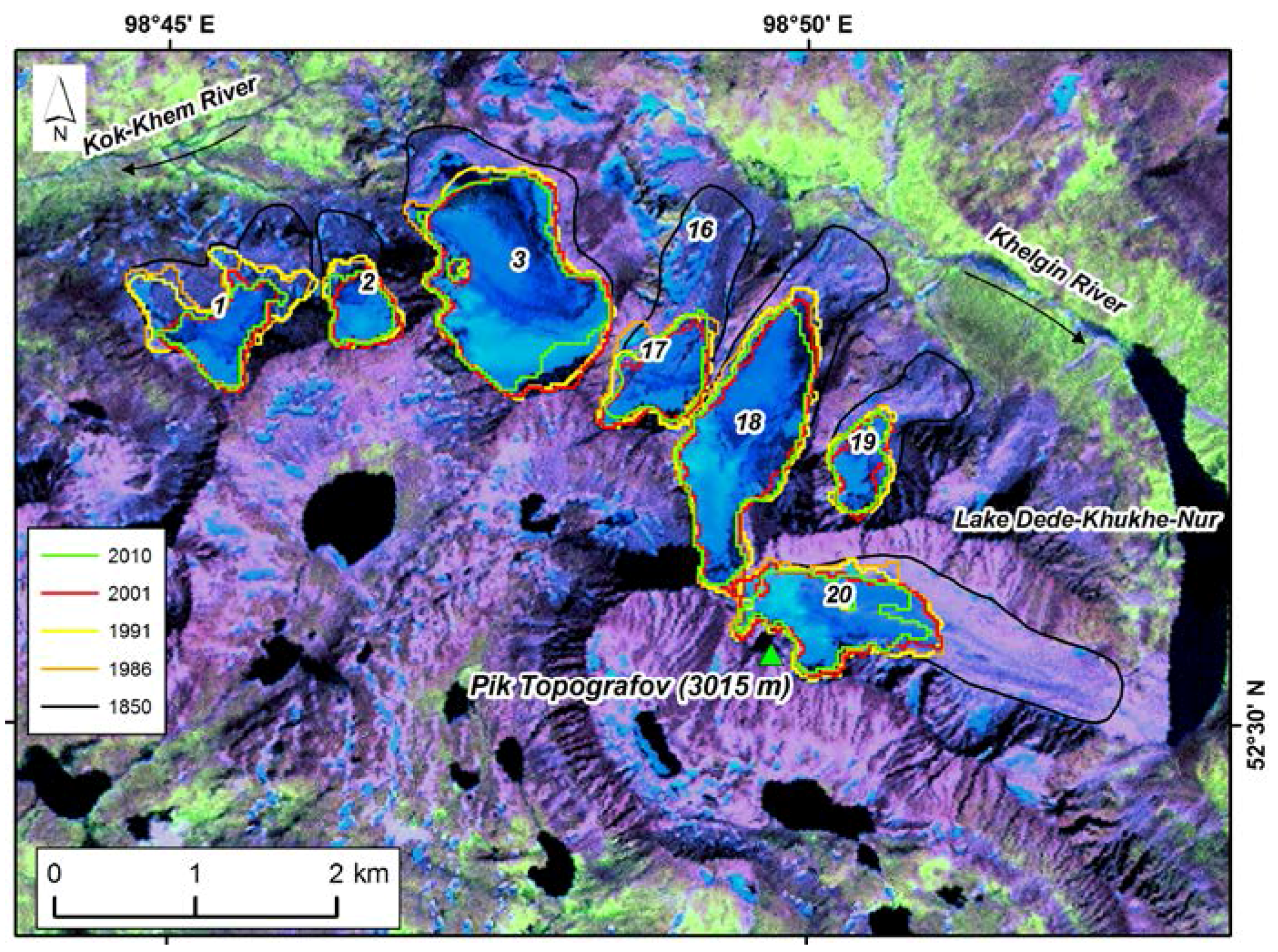
Figure 4.
Glacier extents between 1850 (end of the Little Ice Age) and 2010 in the region of Pik Topografov (the green triangle is in the lower center). The background is a false color composite from Landsat ETM+ (9 August 2001) with bands 5, 4 and 3 (as red, green and blue).
Figure 4.
Glacier extents between 1850 (end of the Little Ice Age) and 2010 in the region of Pik Topografov (the green triangle is in the lower center). The background is a false color composite from Landsat ETM+ (9 August 2001) with bands 5, 4 and 3 (as red, green and blue).

Figure 5.
Relationships (linear regression) between absolute and relative ice area changes (dS) in 1850–2010 and 1991–2010 and initial area (a,b), mean slope (c,d), mean elevation (e,f) and compactness (g,h) of glaciers. The statistically significant relationship (p < 0.05) is indicated by an asterisk.

Figure 6.
Regional time series of total winter (September–May) precipitation and summer (June–August) temperature recorded at the nearest Orlik weather station (for location see Figure 1). The thick line shows the 5-year moving average.
Figure 6.
Regional time series of total winter (September–May) precipitation and summer (June–August) temperature recorded at the nearest Orlik weather station (for location see Figure 1). The thick line shows the 5-year moving average.


Table 1.
Remote sensing data used in this study.
| Glacier Inventory | Path | Row | Satellite/Sensor | Date of Acquisition | Spatial Resolution (m) |
|---|---|---|---|---|---|
| GI1990 | 137 | 24 | Landsat-5/TM | 23 July 1986 | 30 |
| 138 | 23 | Landsat-5/TM | 28 July 1991 | 30 | |
| GI2000 | 137 | 23 | Landsat-7/ETM+ | 9 August 2001 | 15, 30 |
| 137 | 24 | Landsat-7/ETM+ | 9 August 2001 | 15, 30 | |
| GI2010 | 43 | 130 | WorldView-1 | 17 July 2008 | 0.5 |
| 44 | 136 | WorldView-1 | 7 August 2008 | 0.5 | |
| 137 | 23 | Landsat-5/TM | 11 September 2010 | 30 |
Table 2.
Morphology and areas of the study glaciers from 1850 to 2010 (area values are in square kilometres). Adopted accuracy for individual ice area measurements from Landsat based data (1986–2010) is ±10% (see in text).
Table 2.
Morphology and areas of the study glaciers from 1850 to 2010 (area values are in square kilometres). Adopted accuracy for individual ice area measurements from Landsat based data (1986–2010) is ±10% (see in text).
| Glacier | Morphology 1 | Mean Aspect 2 | Mean Slope 2 | 1850 | 1953 1 | 1986 | 1991 | 2001 | 2010 |
|---|---|---|---|---|---|---|---|---|---|
| 1 | cirque-valley | 5 (N) | 23 | 0.932 | 0.6 | 0.592 | 0.576 | 0.306 | 0.285 |
| 2 | cirque | 342 (NNW) | 23 | 0.424 | 0.3 | 0.242 | 0.240 | 0.195 | 0.185 |
| 3 (Avgevich Glacier) | cirque-valley | 342 (NNW) | 13 | 1.966 | 1.4 | 1.498 | 1.467 | 1.372 | 1.238 |
| 17 | cirque-valley | 20 (NNE) | 22 | 0.950 | 0.6 | 0.442 | 0.397 | 0.322 | 0.334 |
| 18 | valley | 12 (NNE) | 18 | 1.621 | 1.2 | 1.145 | 1.139 | 0.973 | 0.983 |
| 19 | cirque | 22 (NNE) | 24 | 0.556 | 0.3 | 0.235 | 0.244 | 0.181 | 0.204 |
| 20 | valley | 70 (ENE) | 19 | 1.654 | 1.3 | 0.785 | 0.761 | 0.660 | 0.543 |
| Sum | 8.103 | 5.7 | 4.939 | 4.824 | 4.009 | 3.772 | |||
| Mean | 1.158 | 0.8 | 0.706 | 0.689 | 0.573 | 0.539 | |||
| Median | 0.950 | 0.6 | 0.592 | 0.576 | 0.322 | 0.334 | |||
1 Total area data from the Catalogue of Glaciers of the USSR [7]. 2 Data relating to 2001 (mean aspect and mean slope figures are in degrees).
Table 3.
Comparison of debris-free glacier areas derived both automatically and manually from TM (on 11 September 2010) and high-resolution WorldView-1 image (on 7 August 2008). Standard deviation was calculated for ten manual digitizations on TM.
Table 3.
Comparison of debris-free glacier areas derived both automatically and manually from TM (on 11 September 2010) and high-resolution WorldView-1 image (on 7 August 2008). Standard deviation was calculated for ten manual digitizations on TM.
| No. of Glacier 1 | Manual on TM | Auto on TM | Auto on TM + Manual Correction | Manual on WorldView-1 | Difference (1)–(4) | Difference (2)–(4) | Difference (3)–(4) | Std. Dev. |
|---|---|---|---|---|---|---|---|---|
| (1) | (2) | (3) | (4) | |||||
| km2 | km2 | km2 | km2 | % | % | % | % | |
| 1 | 0.293 | 0.353 | 0.285 | 0.262 | 12 | 35 | 9 | 4 |
| 2 | 0.202 | 0.185 | 0.185 | 0.180 | 12 | 3 | 3 | 7 |
| 3 (Avgevich Glacier) | 1.324 | 1.304 | 1.238 | 1.319 | 0 | −1 | −6 | 1 |
| 17 | 0.352 | 0.087 | 0.334 | 0.332 | 6 | −74 | 1 | 2 |
| 18 | 1.015 | 0.985 | 0.983 | 0.944 | 8 | 4 | 4 | 2 |
| 19 | 0.214 | 0.204 | 0.204 | 0.187 | 14 | 9 | 9 | 3 |
| 20 | 0.663 | 0.543 | 0.543 | 0.636 | 4 | −15 | −15 | 3 |
| All | 4.063 | 3.661 | 3.772 | 3.860 | 5 | −5 | −2 |
1 Numbering according to the Catalogue of Glaciers of the USSR (GI1950).
© 2018 by the authors. Licensee MDPI, Basel, Switzerland. This article is an open access article distributed under the terms and conditions of the Creative Commons Attribution (CC BY) license (http://creativecommons.org/licenses/by/4.0/).
Share and Cite
MDPI and ACS Style
Osipov, E.Y.; Osipova, O.P. Glacier Changes on the Pik Topografov Massif, East Sayan Range, Southeast Siberia, from Remote Sensing Data. Geosciences 2018, 8, 148. https://doi.org/10.3390/geosciences8050148
AMA Style
Osipov EY, Osipova OP. Glacier Changes on the Pik Topografov Massif, East Sayan Range, Southeast Siberia, from Remote Sensing Data. Geosciences. 2018; 8(5):148. https://doi.org/10.3390/geosciences8050148
Chicago/Turabian StyleOsipov, Eduard Y., and Olga P. Osipova. 2018. "Glacier Changes on the Pik Topografov Massif, East Sayan Range, Southeast Siberia, from Remote Sensing Data" Geosciences 8, no. 5: 148. https://doi.org/10.3390/geosciences8050148
Note that from the first issue of 2016, this journal uses article numbers instead of page numbers. See further details here.