Origin of High Density Seabed Pockmark Fields and Their Use in Inferring Bottom Currents

Abstract

Some of the highest density pockmark fields in the world have been observed on the northwest Australian continental shelf (>700/km²) where they occur in muddy, organic-rich sediment around carbonate banks and paleochannels. Here we developed a semi-automated method to map and quantify the form and density of these pockmark fields (~220,000 pockmarks) and characterise their geochemical, sedimentological and biological properties to provide insight into their formative processes. These data indicate that pockmarks formed due to the release of gas derived from the breakdown of near-surface organic material, with gas accumulation aided by the sealing properties of the sediments. Sources of organic matter include adjacent carbonate banks and buried paleochannels. Polychaetes biodiversity appears to be affected negatively by the conditions surrounding dense pockmark fields since higher biodiversity is associated with low density fields. While regional bi-directionality of pockmark scours corresponds to modelled tidal flow, localised scattering around banks suggests turbulence. This multi-scale information therefore suggests that pockmark scours can act as proxy for bottom currents, which could help to inform modelling of benthic biodiversity patterns.

1. Introduction

Pockmarks are seafloor depressions that form in soft sediment by fluid-flow processes. They have been reported since the 1970s [1] and are present worldwide [2]. Pockmarks are most commonly found in areas of thick Holocene sediment accumulation along continental shelves, in tropical to glacial settings. The expression of fluid-flow via pockmarks at the seafloor is important for several reasons. These include the need to identify potential hydrocarbon resources and areas where carbon sequestration is not possible due to the potential leakage of the targeted reservoir [3]; areas of potential geohazards (e.g., gas venting, slope failure, basement faulting) [4,5]; and areas of significant biodiversity associated with seep-related habitats, such as bioherms and reefs [1,6,7].

Pockmarks have been observed aggregated in low to very high density pockmark fields, such as the ~900/km² observed in the Barents Sea, Norway [8], and in both a random and non-random distribution due to the presence of underlying faults or buried paleo-channels [2]. Pockmarks range in size over almost four orders of magnitude (decimetres to km diameter), with mega-pockmarks (>3 km diameter) observed in the South China Sea [9], but are most commonly observed with diameters of the order of in the tens to hundreds meters [2]. Their vertical relief ranges from decimeters to about 30 m. Pockmarks tend to have distinct v- to u-shaped profile, a variable shape in plan view, and outline that can be circular or elongated in shape due to modification by seabed currents [10].

Pockmarks can be maintained through the semi-continuous fluid or gas escape, a lack of sedimentation to infill them or self-maintenance and scouring caused by local turbulence created when currents flow over them [11,12]. Pockmarks may affect faunal abundance or biotic composition through differences in environmental parameters (sedimentology, geochemistry, boundary layer dynamics, oxygen saturation) between pockmarks and surrounding areas [13,14,15,16]. Research on the infaunal communities of the Bonaparte Basin (offshore northern Australia) have shown distinct polychaete assemblages on sediment plains compared to other geomorphic features, but there was no investigation of the possible relationships to pockmarks [17].

Analysis of pockmark morphology and spatial distribution in relation to seabed geological and oceanographic processes can provide insight into the processes driving their development, the sub-seabed plumbing system and their potential influence on infaunal distribution [2]. With the growing use of multibeam sonar to image the seafloor at very high-resolution, small pockmarks clustered in large concentrations are more commonly observed. Characterising these consistently and efficiently can be challenging, thus several semi-automated digital mapping methods have been recently developed [18,19,20].

This paper has the following objectives:

(1)

Identify and map pockmarks on the shelf of the western Timor Sea, Australia using a new semi-automated method.

(2)

Document the geochemical and sedimentological properties of pockmark sediments, and of associated infaunal communities.

(3)

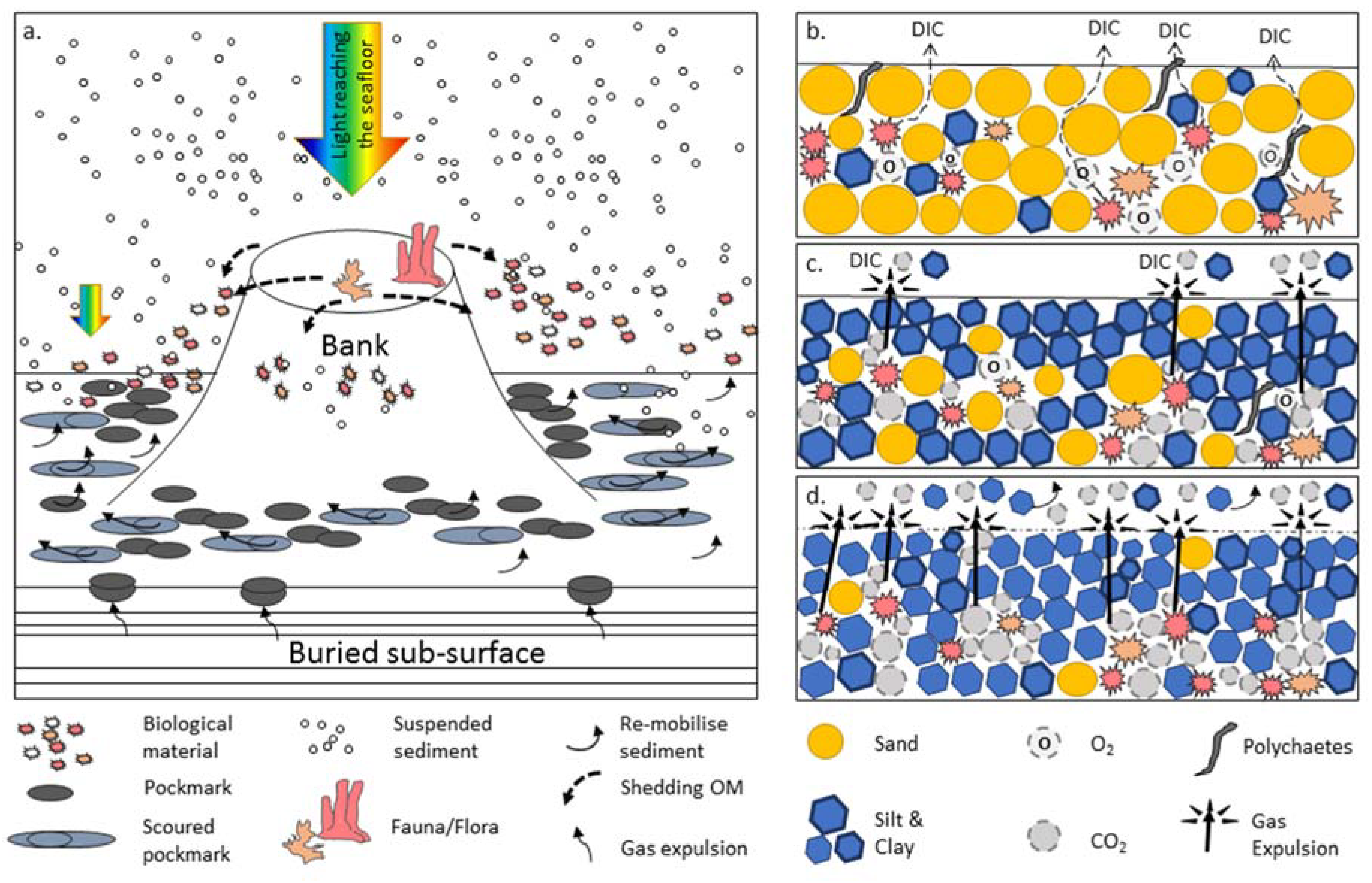
Present a conceptual model for pockmark formation that links pockmark form and density to local environmental conditions, including hydrodynamics and sedimentary processes.

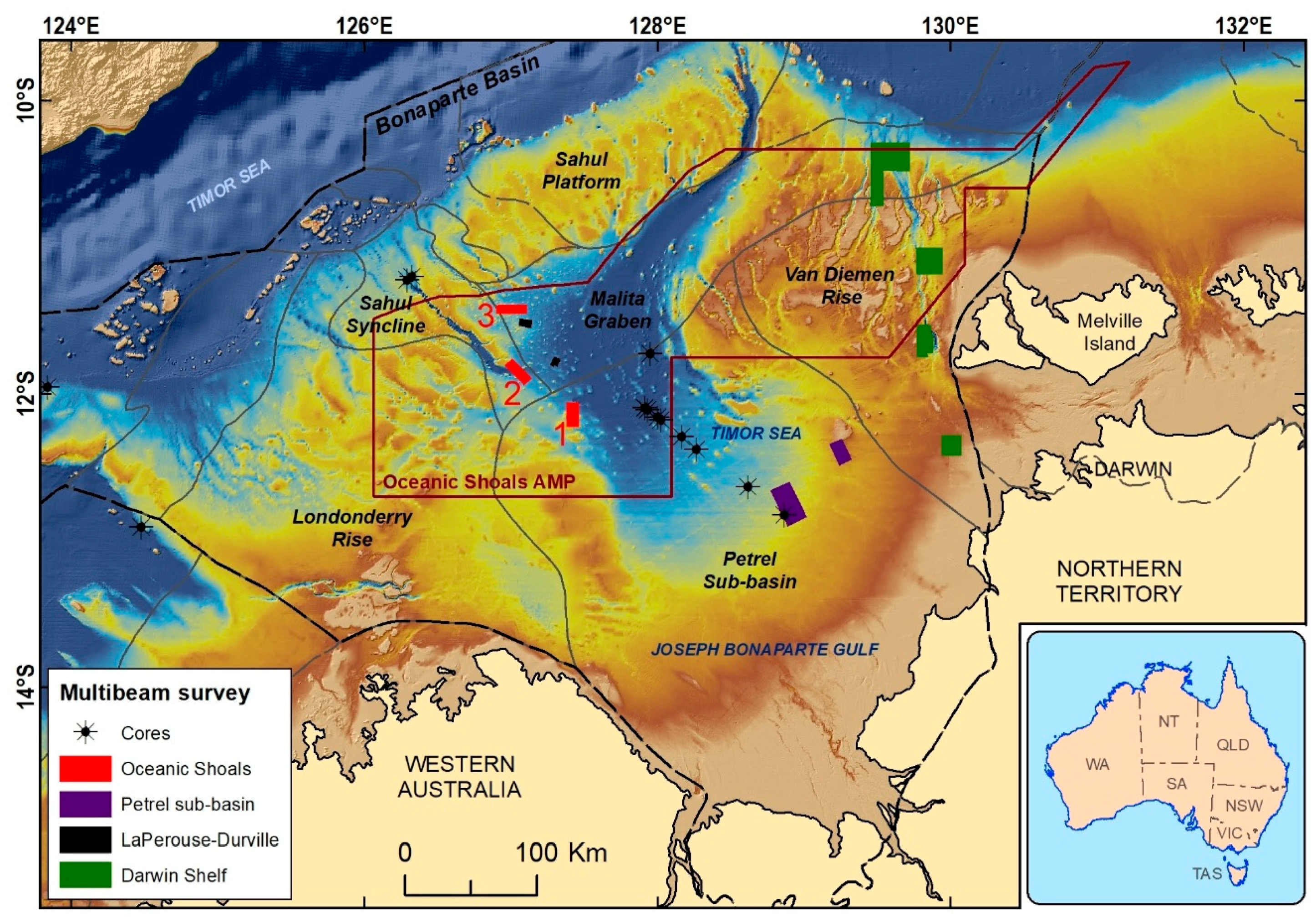
1.1. Regional Setting

1.1.1. Geological and Physiographic Settings

The study area is located in the tropical Oceanic Shoals Australian Marine Park (AMP; 71,740 km²) within the Timor Sea on the continental shelf of northwestern Australia. The area lies within the sedimentary Bonaparte Basin, which is expressed at the seabed by the Van Diemen Rise, Sahul Shelf, Malita Graben, Sahul Syncline, Petrel Sub-basin and the Londonderry Rise (Figure 1). The Sahul Shelf, Van Diemen Rise and Londonderry Rise form carbonate-dominated platforms characterised by a complex suite of submerged flat-topped carbonate banks and terraces, separated by valleys, channels and plains [21,22,23,24,25]. Water depths range from 10 m on the shallowest banks to over 200 m in shelf-incising valleys. The central basin is about 270 km long with water depths of 90 to 140 m. The seabed of the greater Bonaparte Basin, including the Oceanic Shoals AMP region represents a drowned landscape consisting of coastal lowlands, estuarine valleys and nearshore environments. These are the product of periodic and repeated formation of a semi-enclosed sea during the Quaternary and most recently inundated during the Late Pleistocene to Holocene postglacial rise in sea level [26,27,28].

1.1.2. Environmental and Oceanographic Settings

The Oceanic Shoals study area is within a tropical region, with a pronounced southern hemisphere summer monsoonal season that commonly includes cyclones. The Indonesian Through-Flow, passing between Timor and northern Australia delivers relatively warm (~26 °C to 31 °C) low salinity water from the north. Across the shelf, macrotidal conditions drive strong tidal flows and wind-driven waves and seasonal cyclones come from the east. These conditions result in an anticlockwise ocean circulation across the shelf strongly influencing sediment transport [30]. The re-suspended seabed sediments coupled with sediment discharged from coastal river systems, contribute to a turbid shelf environment that is likely to suppress photosynthetic activity at the seabed. This therefore may be an important determinant of the composition of benthic assemblages across the region [31].

The study area encompasses three areas located along the north and west portion of the central basin (Figure 1). Of these, Area 1 is located within the Petrel Sub-basin, Area 2 straddles the southern portion of the cross-shelf valley within the Sahul Syncline (Figure 1), and Area 3 is located across the Sahul Syncline to Malita Graben transition. The extent of this general area spans a cross-shelf transect of approximately 110 km (Figure 1). Each area was positioned to encompass a variety of seabed geomorphic features and water depths, as identified in the national geomorphic features database [21,23].

On most of the Australian continental shelf, pockmarks are seldom found because of the dominance of coarse sediments (sand and gravel) in most regions. There is also a limited input of terrigenous organic–rich sediments, and a moderate to high percentage of carbonate sediments on the shelves [27,30]. However, high-density fields of pockmarks are present within the broad continental shelf of northern Australia, including the extensive Bonaparte Basin where seabed sediments do incorporate terrigenous fine-grained material. During the Quaternary, the present seabed of the Bonaparte Basin has been repeatedly exposed either in part, or completely, from eustatic sea level changes [27,28,32]. During low sea-levels, banks, shoals and terraces became exposed, resulting in Joseph Bonaparte Gulf forming a semi-enclosed basin [33]. Within the Bonaparte Basin, the Petrel Sub-basin, Malita Graben, Sahul Syncline and adjacent structural elements have acted as a depocentre for marine and riverine sediment since the Paleozoic [26,27,33,34,35,36]. This resulted in hydrocarbon generation occurring at depths in older sedimentary strata. Recently, seabed sediment with a particularly high organic matter content derived from the preservation of mangroves and other plant matter has been reported within paleo-river channels mapped on the Petrel Sub-basin mid-shelf and presently covered by a thin sediment veneer [33]. Additionally, the reworking of buried terrestrial sediments upwards to the seabed via pockmark formation has been identified within the Petrel Sub-basin using rare earth element chemistry [37]. Previous studies suggested that banks of the greater Oceanic Shoal region could result from one of these two processes: (1) hydrocarbon release from depth and its movement upward in faults providing a food source for the colonising reef-builders, or (2) thinner sediment cover over organics resulting in faster release of the product of organic breakdown [29].

2. Materials and Methods

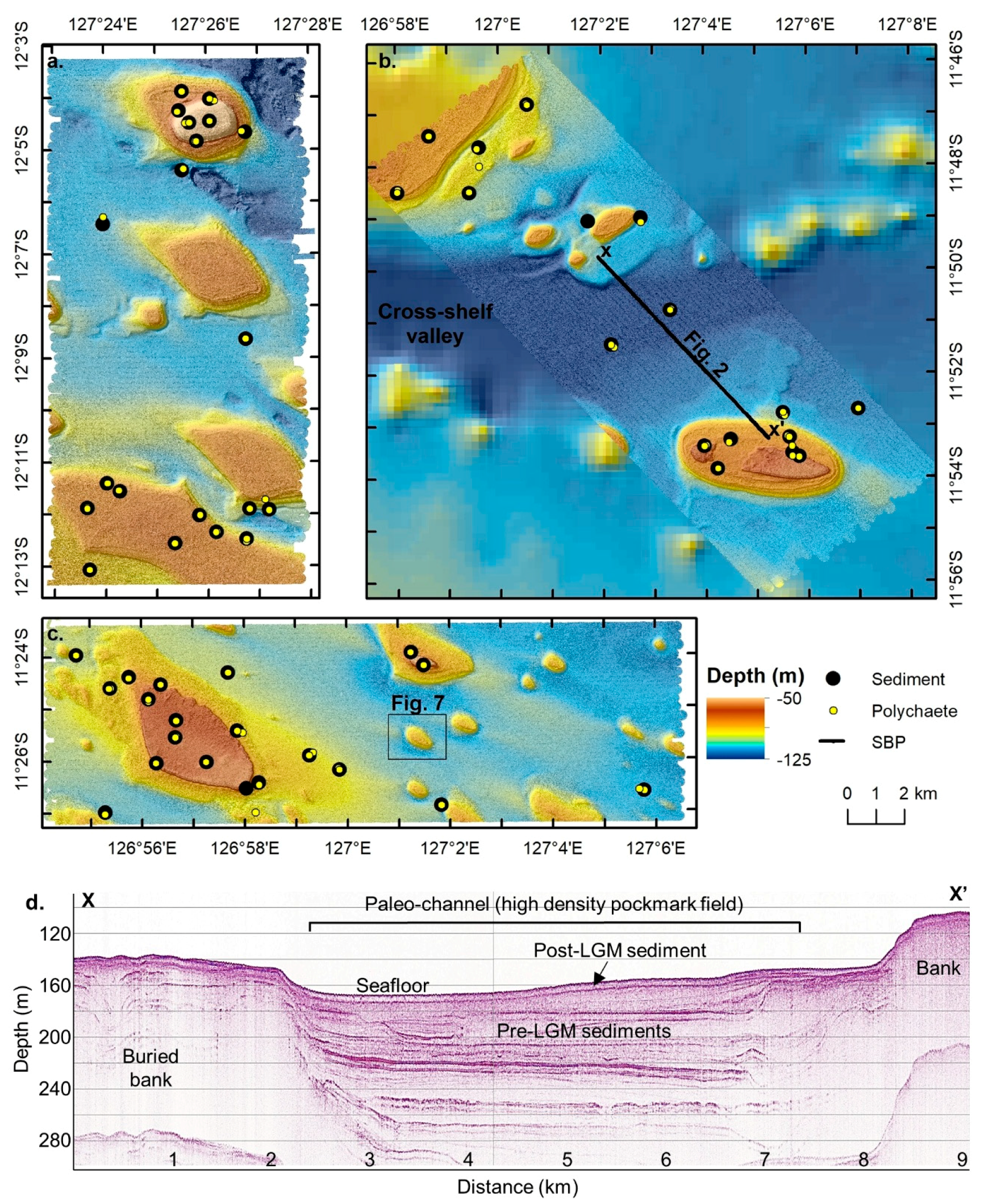
2.1. Survey Summary

The data presented herein were collected during the Oceanic Shoals environmental marine survey (SOL5650/GA0339) undertaken in September 2012 [21]. High-resolution multibeam echosounder (MBES) bathymetry and backscatter data were collected over three areas covering a total of about 425 km² of seabed (Figure 1). MBES bathymetric data was processed using Caris Hips and SIPS v.7.1. Seabed backscatter data was processed with CMST-GA MB Process toolbox software co-developed by the Centre for Marine Science and Technology at Curtin University of Technology and Geoscience Australia [38]. Both data types were gridded at 1 m horizontal resolution for analysis and interpretation purposes.

Shallow sub-bottom profiles (SBP) were collected over 140 line km using a sparker source and processed with a C-view processing unit using 1 sec firing rate and 500 ms record length, then filtered using band-pass filter and converted to SGY file. Seabed samples were collected in duplicates at 61 stations using a Smith-McIntyre grab or box corer (Figure 2). Each sample was analysed for sedimentological characteristics (sediment texture as Mud, Sand and Gravel %, grain-size distribution, CaCO₃ content) and geochemical composition (incl. porosity, CO₂ production rates (TCO₂), and Total Organic Content (TOC)) as described in [21,39] method, and polychaetes biodiversity (57 stations only—identified to species level according to [17]).

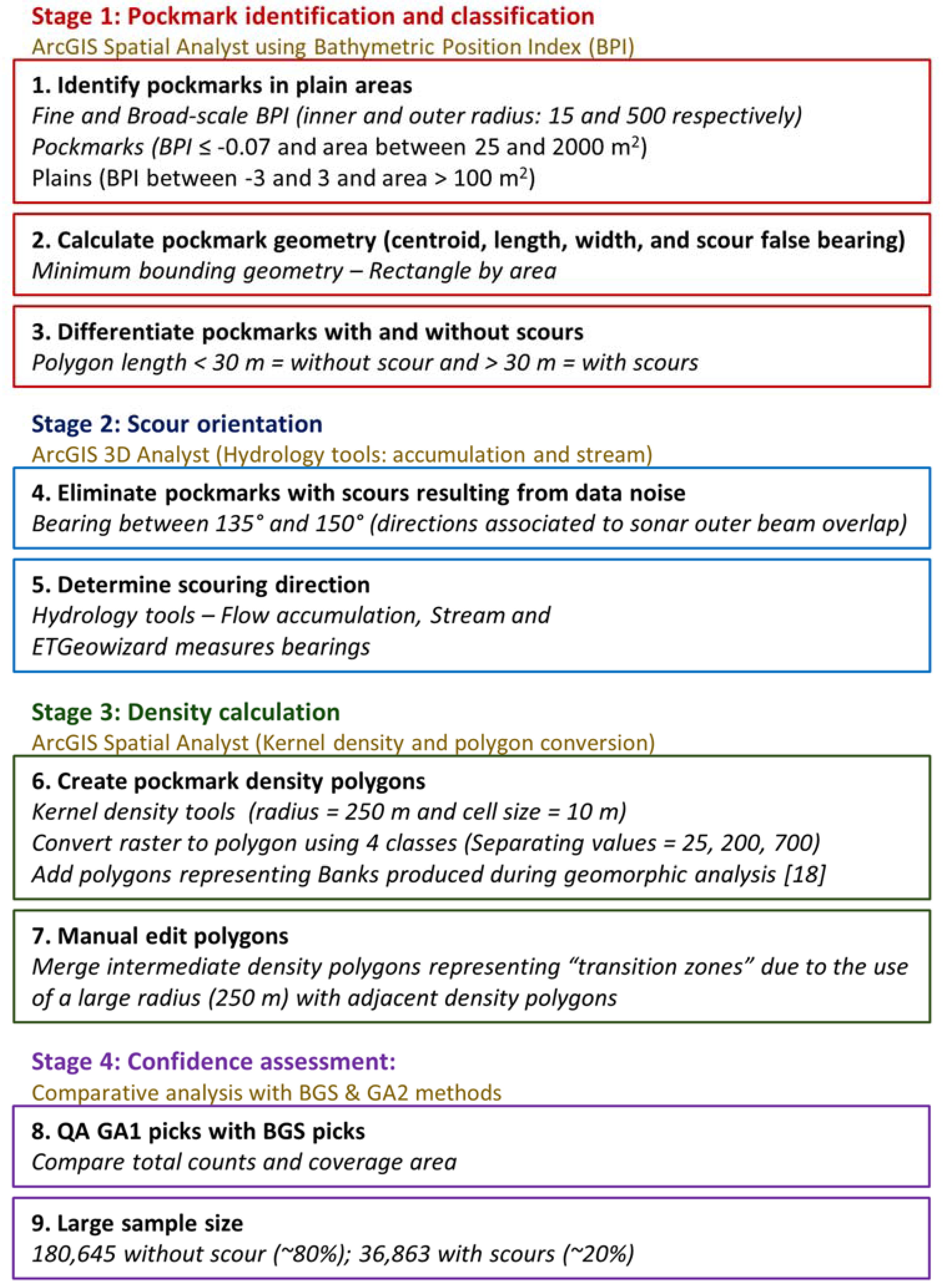
2.2. Geomorphic Analysis and Automated Pockmarks Characterisation

Geomorphic feature mapping was completed manually using MBES data and derivative datasets such as slope and contour to identify discrete features (Figure 3) [21]. Feature definitions were based on [23]. For this study, bank morphometric profiles were calculated using ArcGIS 3D (v. 10.1, Esri, Redlands, CA, USA) profiling across the narrowest axis of the bank (Figure 3b).

Due to their large number, manual mapping of individual pockmarks was deemed unsuitable. Therefore, an automated method (GA1) was developed to identify both pockmarks and associated scour marks. The overall approach was similar to other published automated and semi-automated methods [10,18], in which a multi-stage process was undertaken. The main stages included (1) identifying pockmarks and differentiating scoured from non-scoured pockmarks, (2) determining scour orientation, (3) calculating field density and (4) assessing confidence in the results (Figure 4). Each step of the method used an existing suite of ESRI spatial analytical tools, such as the hydrological and surface toolboxes. Details of the method can be found in the supplementary material. Density classes were used as a common unit for comparative analyses with other survey datasets.

The pockmarks identified using the GA1 method were compared with results from two other methods using a small subset area of Area 3. These methods were a combination of the British Geological Survey (BGS) Seabed Mapping toolbox [18,20] and the Geomorphometry and Gradient Metrics (GGM) toolbox [40], and another tool tested by Geoscience Australia (GA2). The subset area included a carbonate bank and the associated clustered pockmarks surrounding its base, as well as other scoured and non-scoured pockmarks distributed in the plain area.

For the BGS combined approach, the landform tool in the GGM toolbox was used to create the surface curvature landform index (Bolstad’s variant) using a square neighborhood analysis window of 12 by 12 cells. The derived raster was used as input for the Feature delineation [Derived] tool within the BGS Seabed Mapping Toolbox [20]. The mapped features corresponded to the areas with a surface curvature landform index lower than −0.04, that are wider than 5 m with a minimum size ratio higher than 0.2 and that include cells with values lower than −0.05. The final outline was achieved by adding a 2 m buffer.

The GA2 method shared similarities with BGS approach, in which Hydrology toolset in ArcGIS^TM was used to identified sinks and pits from the bathymetry data. However, GA2 used a fuzzy features tool in landserf (based on topographic terrain analysis) to calculate multiscale pitness [41] and the openness tool (based on the viewshed principle) to calculate positive openness [42]. Both calculations were based on a search radius of 21 cells. Where pitness was greater than the mean plus one standard deviation, pits were identified. From these, only the ones associated with a positive openness values of less than the mean minus one standard deviation were selected and converted into polygons (simplify boundary function ON). Selection was further constrained by only selecting polygons that intersected either sinks, or pits or both. Finally, polygons with area less than 10 m² were deleted and resultant polygons were regarded as pockmarks. The key issue related to these semi-automated methods is the choices of value thresholds, which is a somewhat subjective process.

2.3. Infaunal Data Analyses on Grab Samples

Multivariate analyses were performed only on samples that returned polychaetes identified to species level, while univariate analyses of species richness and abundance included samples from which no polychaetes were identified. All samples from banks were excluded from statistical analyses because these did not have an associated value for pockmark density. Assemblage data and species richness data were square-root transformed to reduce the influence of dominant groups [43] and meet ANOVA assumptions, respectively. A PERMANOVA using unrestricted permutation of raw data and type III SS [44] was undertaken to determine if polychaete assemblages varied among pockmark density classes, while a 1-way ANOVA was undertaken to determine if species richness varied among pockmark density classes.

2.4. Hydrodynamic Model

To understand the processes contributing to the presence of pockmarks and associated scouring, a coastal shelf model was constructed to evaluate bed shear stress at the three different survey areas (Figure 1). A finite element model utilising an unstructured grid was constructed. The bathymetry used in the model was Australian Bathymetry and Topography Model [45] gridded at 250 m and the multibeam dataset used here gridded at 10 m resolution.

The boundary of the model was set beyond the shelf break in order for the currents to stabilise by the time they reach the study area. The northern boundary conditions were set as open water boundaries between islands of the Indonesian archipelago and Papua New Guinea. Both the eastern and western boundaries were set as open water. Two types of ocean boundary conditions were trialed and both included the semi-diurnal tides. (1) Tidal elevations derived from the TOPEX/Poseidon satellite altimetry global tidal model driver (TMD) toolbox version 2.05 with all constituents implemented to create hourly tidal elevation files, and (2) tidal currents derived from the same toolbox using all harmonic constituents. These currents were multiplied by the width and depth of the boundary to calculate the hourly flow rate. Wind stresses from the Bureau of Meteorology gridded datasets were also applied in both of the seasonally dominant directions of the North West and South East. The wind forcing, while changing the surface currents, did not change the currents near the sea bed and the bed shear stress calculations. The model was refined near the study area and, with salinity kept constant, run for a three-month period to represent mean tidal conditions. From these model runs, the bed shear stress time series and exceedance of erosion was also calculated.

3. Results

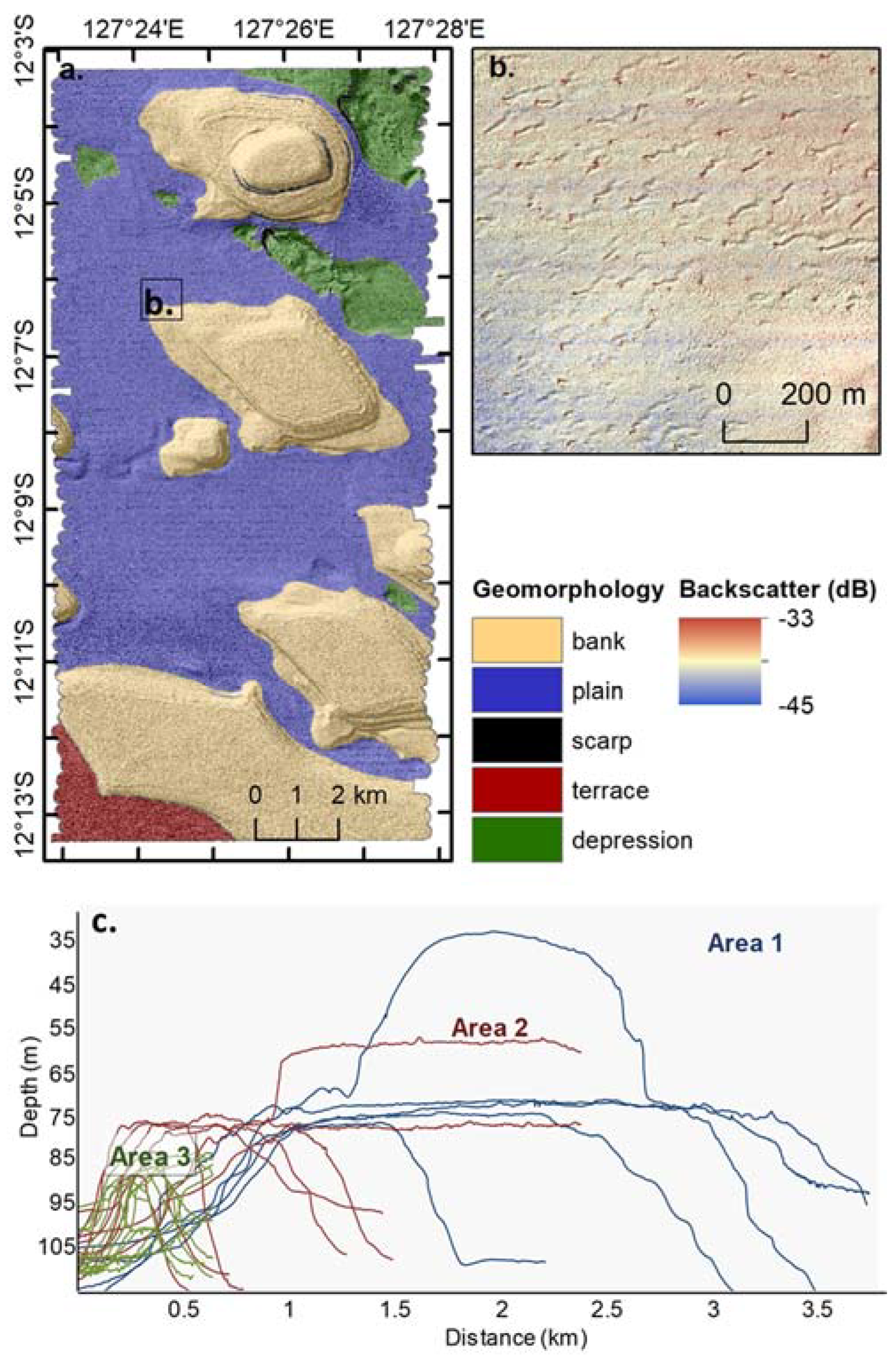
3.1. Geomorphic Analysis

High-resolution seafloor mapping revealed multiple carbonate banks rising tens of meters above otherwise flat pockmarked plains [21].

3.1.1. Banks

Relatively steep-sided (slopes up to 35 degrees) and flat-topped banks are located in water depths of 45 m to123 m (Figure 2). Along their flanks, banks have terraces of various widths, which are regarded as possible indicators of lower sea levels. Banks and their associated features are characterised by the highest backscatter intensity values measured from the multibeam sonar data and coarsest sediment composition sampled [21]. Sub-bottom profiles reveal a mostly acoustically transparent seismic facies across the banks (Figure 2). The dimensions (length and height) of the banks reduces northward towards the shelf edge (Figure 3).

3.1.2. Plains

Plains dominate the seascape, occur between 94m and 146 m water depth and deepen northward. They record gradients averaging 2.5 degrees and are characterised by low backscatter intensity values, representative of the fine-grained sediment observed in the samples [21]. Their sub-surface is mostly characterised by a thick sequence (>150 ms TWT) of acoustically transparent seismic facies closest to the seafloor, underlain by a semi-stratified facies, which in places is replaced by cut and fill facies (Figure 2d). The thickest section (>350 ms TWT) is recorded in the deepest region of Area 2, which corresponds to the start of a deep cross-shelf valley (Figure 1 and Figure 2).

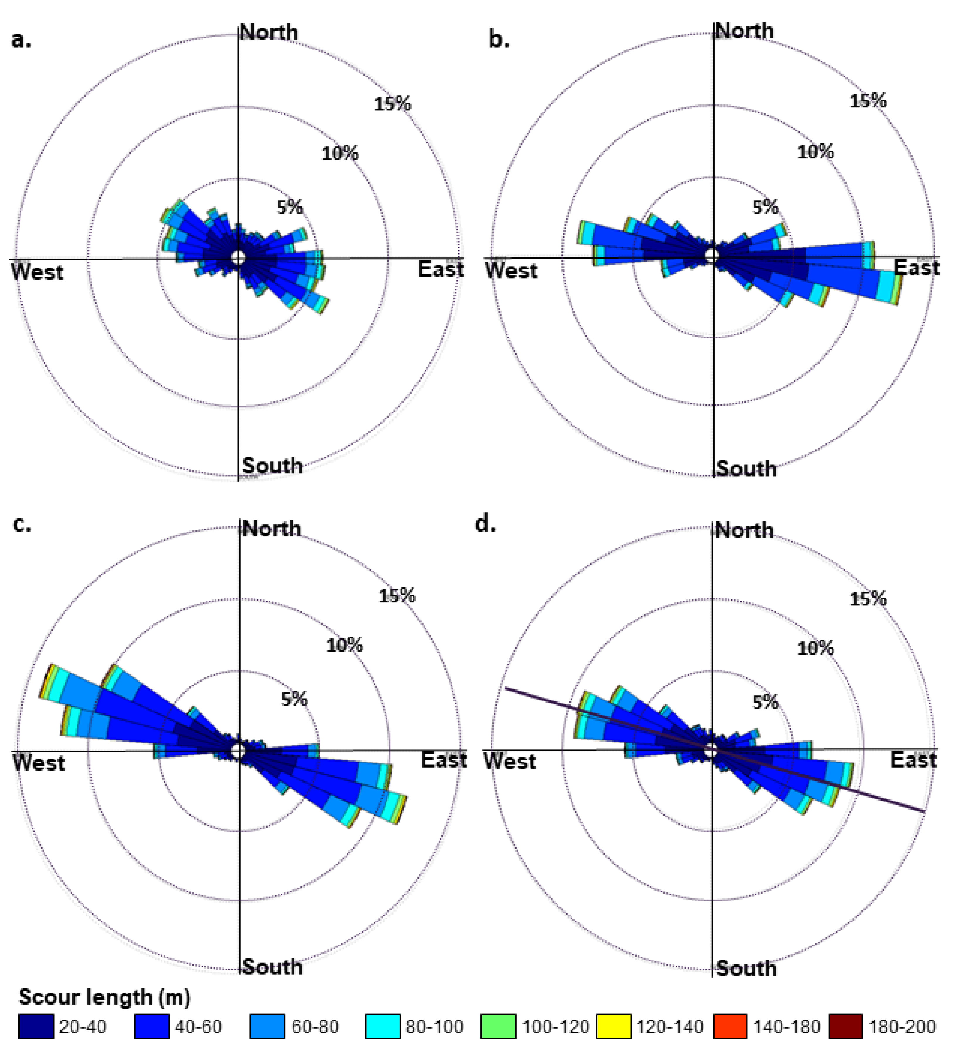
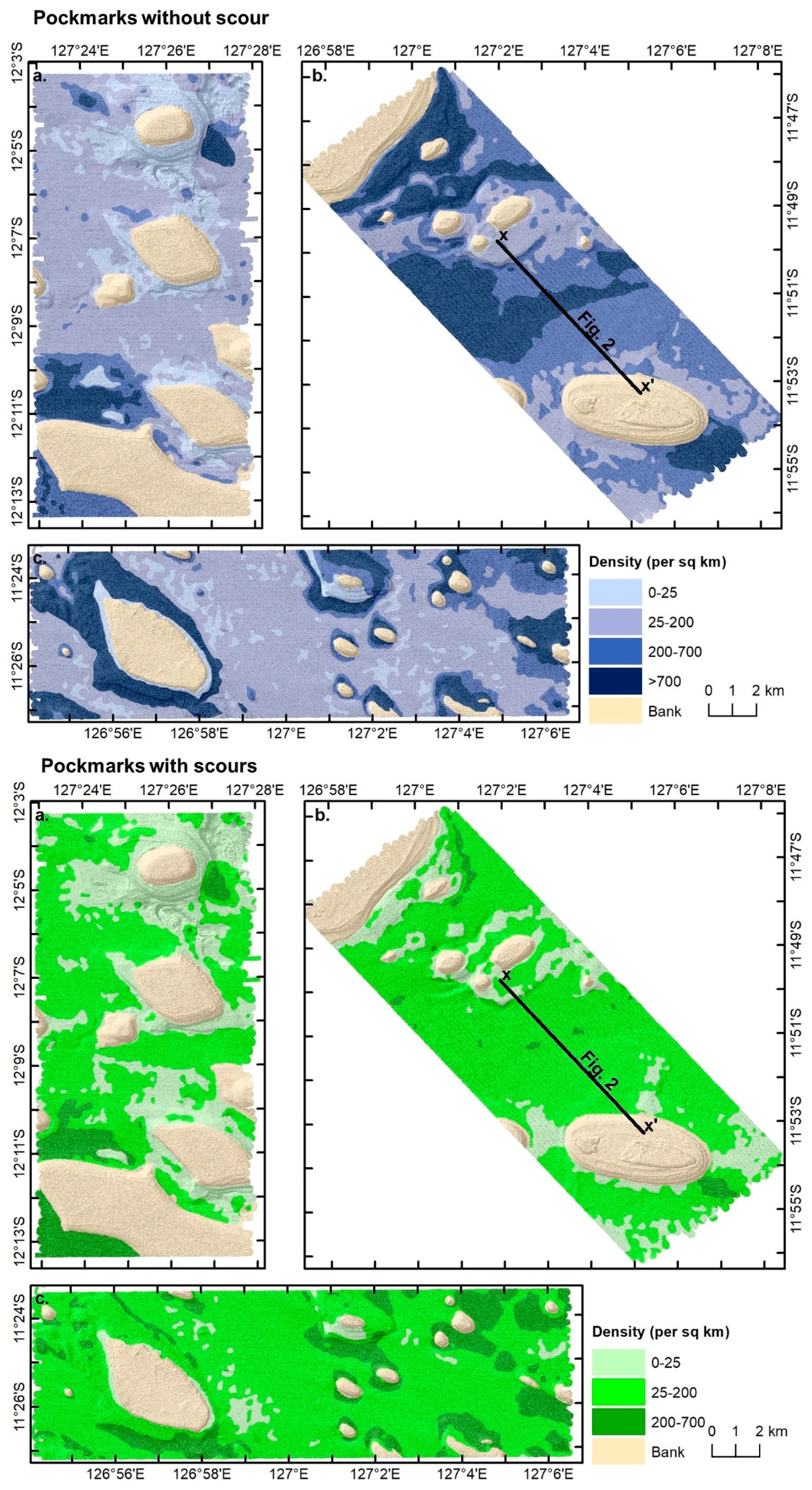
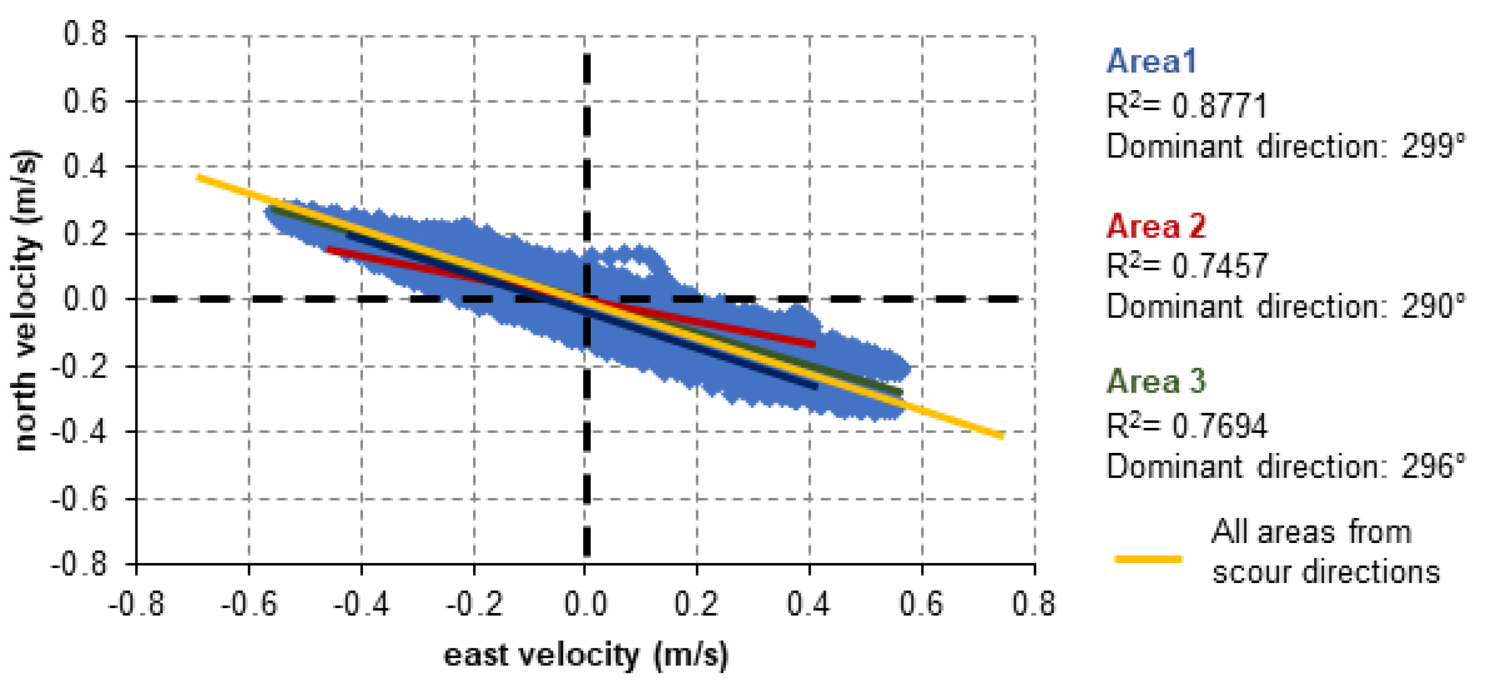
3.1.3. Pockmarks: Density, Scour Direction Results

Semi-automated mapping identified 220,508 pockmarks throughout the plain areas, including at the foot of the banks. Some bank tops also hosted pockmarks, but these were not included in this analysis. Pockmarks displayed wide ranging geometries, varying from circular to elongate. Their dimensions varied from 10 to 30 m in diameter and 0.5 to 2 m in depth. In most cases, the centers of the pockmarks recorded higher backscatter intensity values than their surroundings [21].

Elongated pockmarks represented mainly pockmarks accompanied by a semi-linear depression shallowing in a particular direction (Figure 3b). The depression, commonly but not always, formed a v-shape on the seabed, with the open end of the ‘v’ on the downstream side of the pockmark. These depressions extended for up to ~200 m, but on average less than 80 m, and are interpreted as a scour mark (Figure 5). For the purpose of this study, pockmarks are divided in two main types: with and without scour. Pockmark types are intermixed throughout the areas they are found within and pockmarks without scour are at most 4.5 times more common (see supplementary tables). Scoured pockmarks show strong bi-directionality, which is associated with an overall east-west quadrant ratio of ~1 (Figure 5). The scour directions in Areas 1 and 2 are slightly more biased towards the eastern quadrant, whereas the directions recorded in Area 3 dominate the western quadrant. More specifically, the bi-directionality is strongest in Area 3, with over 75% of the scour directions divided relatively equally between W-NW and E-SE quadrants, while Area 1 is the most scattered (44% within the W-NW and E-SE quadrant; Figure 5 and supplementary tables).

Pockmarks form fields of dense clusters, with densities greater than 700/km² for non-scoured pockmarks (Figure 6). High-density areas are mostly concentrated around the foot of the banks and represent over 17% of the total surveyed area (supplementary Figure S2). The most common density for both types of pockmarks is between 25 and 200/km². Area 1 contains the highest coverage of banks and low density pockmark fields (<25/km²; Figure 6 and supplementary Figure S2). Area 2 contains a large field of high density pockmarks within the cross-shelf valley (Figure 2 and Figure 6) and the largest area of intermediate-density (200–700 pockmark/km²) fields of non-scoured pockmarks (Figure 6 and supplementary material). Many of the scoured pockmarks in the central plain of Area 2, which extends across the southern end of the Sahul Valley (Figure 1), are oriented so that a flow from north to south is indicated for the Sahul Valley. This is consistent with the general anticlockwise circulation suggested for the basin [15]. In Area 3, dense non-scoured pockmarks fields surround the banks and similarly to Area 2, many of the pockmark scours are oriented such that a flow from northwest to southeast is implicated, also consistent with the anticlockwise circulation [30].

3.1.4. Comparison Analysis and Confidence Assessment

Comparison analysis between the results of GA1, GA2 and BGS methods shows that all three methods identified most pockmarks present, within 10% of each other (Figure 7). However, discrepancies exist between their pockmark total count and coverage area (Figure 7i). For example, BGS method identifies 60% more pockmarks than the GA1 method (Figure 7i), but their total coverage areas are similar. These discrepancies are attributed to GA methods often combining closely spaced pockmarks or identifying pockmark scours. For GA1 method, this resulted respectively in reducing the overall pockmark count while increasing the total coverage area (Figure 7i).

3.2. Seabed sediment sample analyses

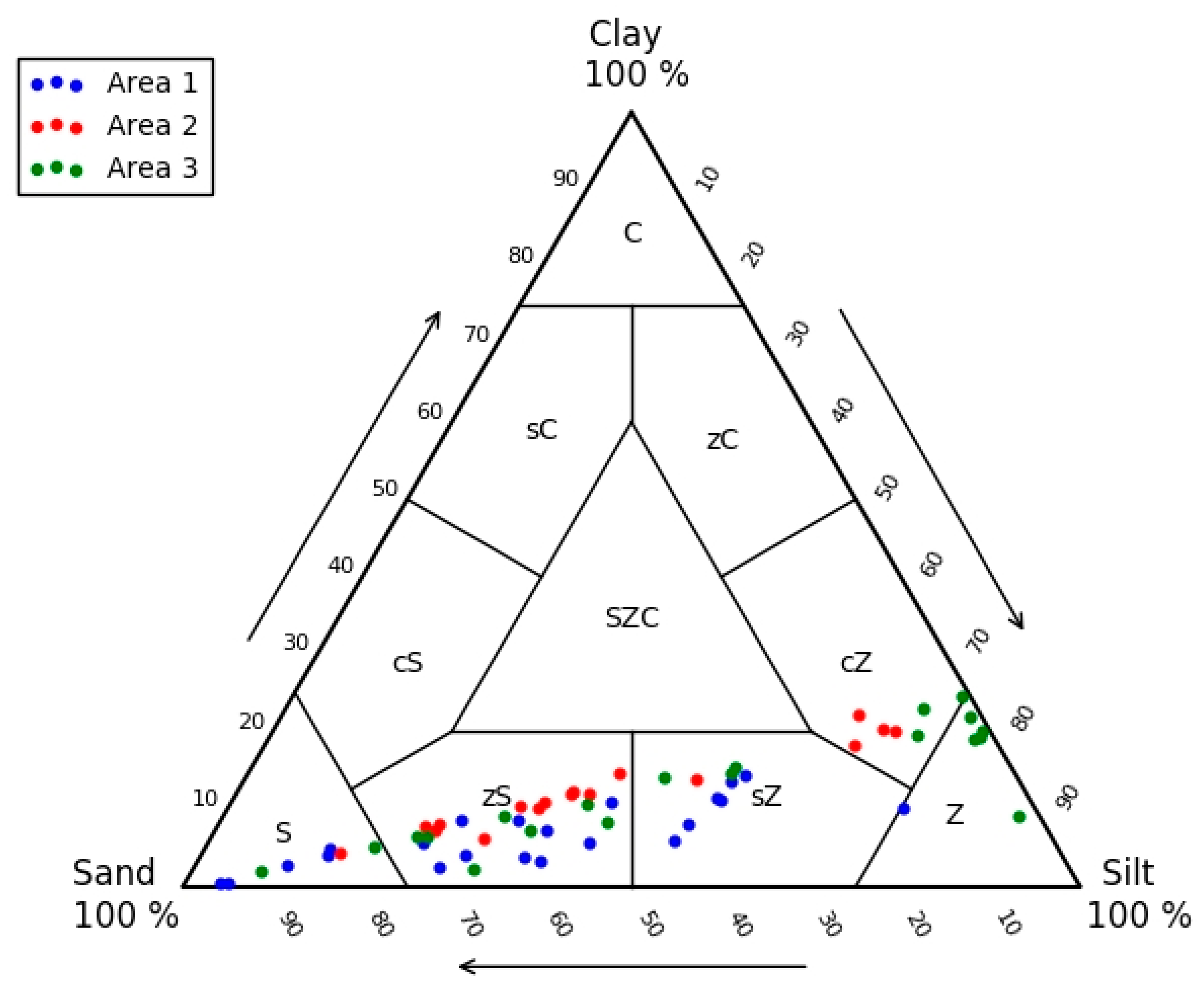
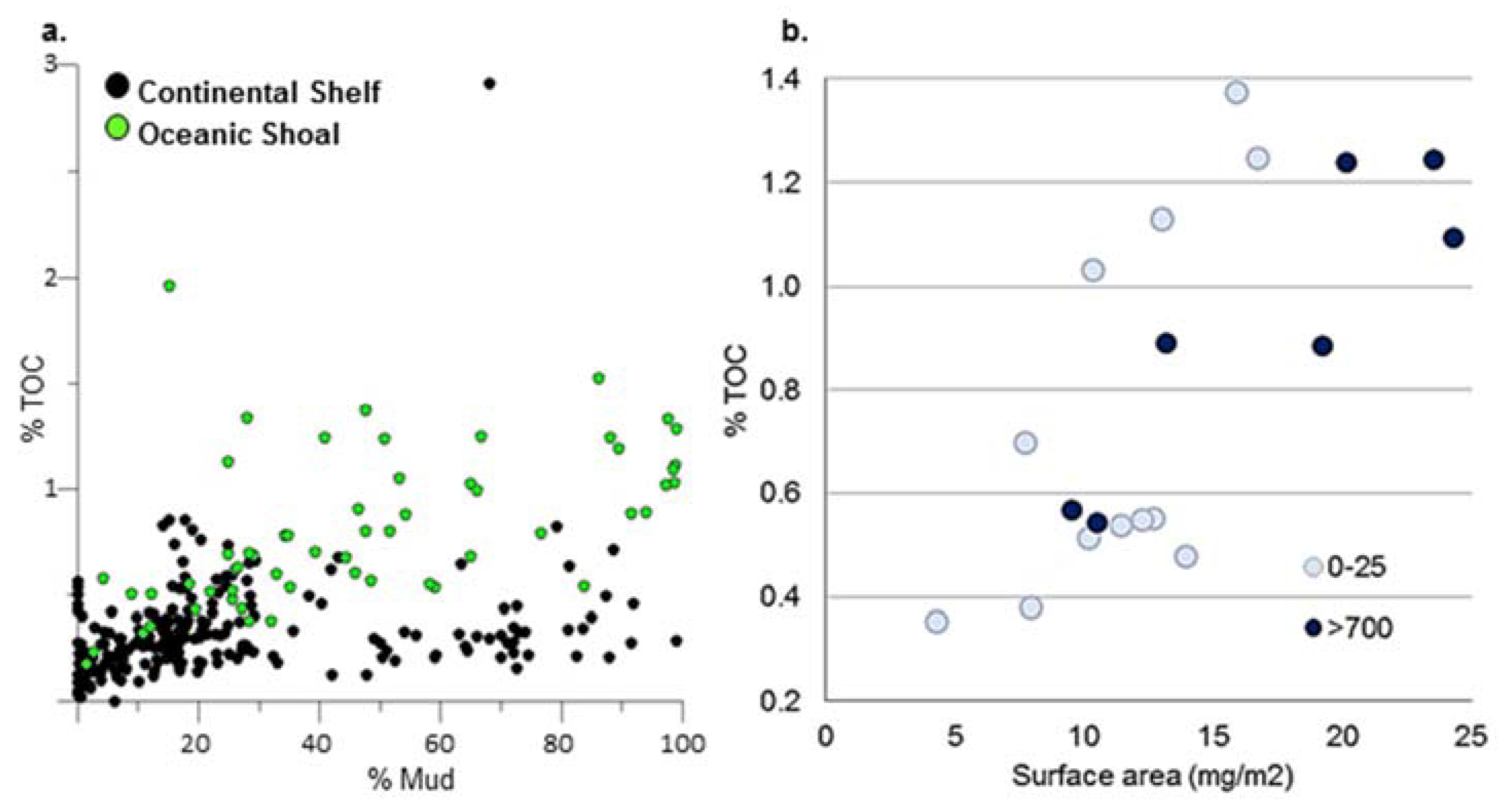
3.2.1. Sediment Texture Analyses

Sediment textures provide some insight into pockmark development. Seabed sediments in the mapped areas have mixed textures, including carbonate-dominated sand (90–95% CaCO₃) and gravel (~95% CaCO₃), and calcareous mud (CaCO₃ values around 25–35%). Some of these sediment samples have the highest mud concentrations measured from the Australian continental shelf [40]. Most of this mud is composed of silt-sized particles, with clay content up to ~25% (Figure 8). The clay is expected to be about 50% smectite, based on data from seabed sediments in the Eastern Joseph Bonaparte Gulf [46]. Low-density pockmark fields have the lowest mud content and highest sand content (Figure 9). This relationship reverses for higher density fields but mud content is greatest in the plain areas where pockmark densities are less than 200/km². Gravelly mud and muddy gravel generally occur where the highest pockmark field densities are found (i.e., foot of the banks), with the mud to sand ratio less pronounced than for the plains (Figure 9). These textural relationships are also directly correlated with the average seabed backscatter intensities, in which the highest backscatter intensities are associated with the banks and where the sand to mud ratio is greater than 1. The opposite relationship is observed for the areas of lowest backscatter intensities (Figure 9).

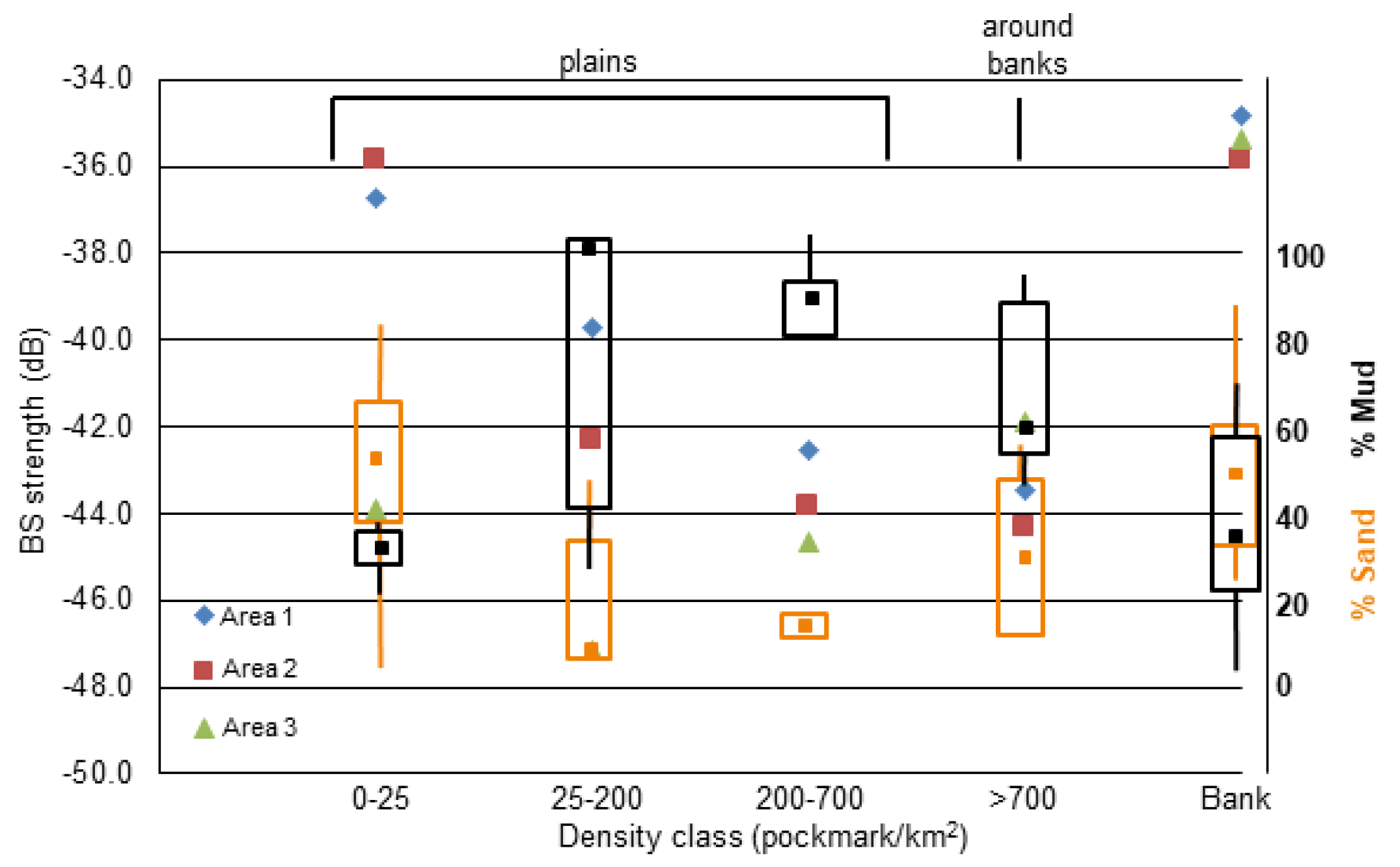
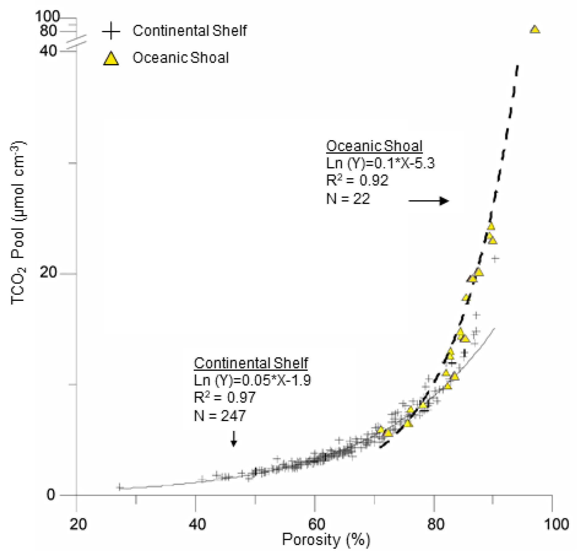
3.2.2. Geochemistry Analyses

Oceanic Shoals sediments have the highest Total Organic Carbon (TOC) concentrations of sediments collected so far on the Australian continental shelf, which average 0.8% (Figure 10a, [39]). Moreover, there is a positive linear relationship between the mud content, surface area (SSA) and TOC as common for Australian Shelf sediments [48]. While most Oceanic Shoals sediments have surface area-normalised TOC concentrations that are in the typical range for the continental shelf [39], the sediments from the dense pockmark fields have less TOC per unit surface area than sediments from the low-density pockmark fields (Figure 10b).

When organic matter breaks down in marine sediments, dissolved inorganic carbon (DIC) is released to porewaters where it may build up in concentration. Porewater DIC concentrations of seabed sediments on Australia’s continental margin (as TCO₂ pool) increase approximately exponentially with porosity, and the slope of this relationship is about two-fold higher for pockmarked sediment of the Oceanic Shoals area (Figure 11).

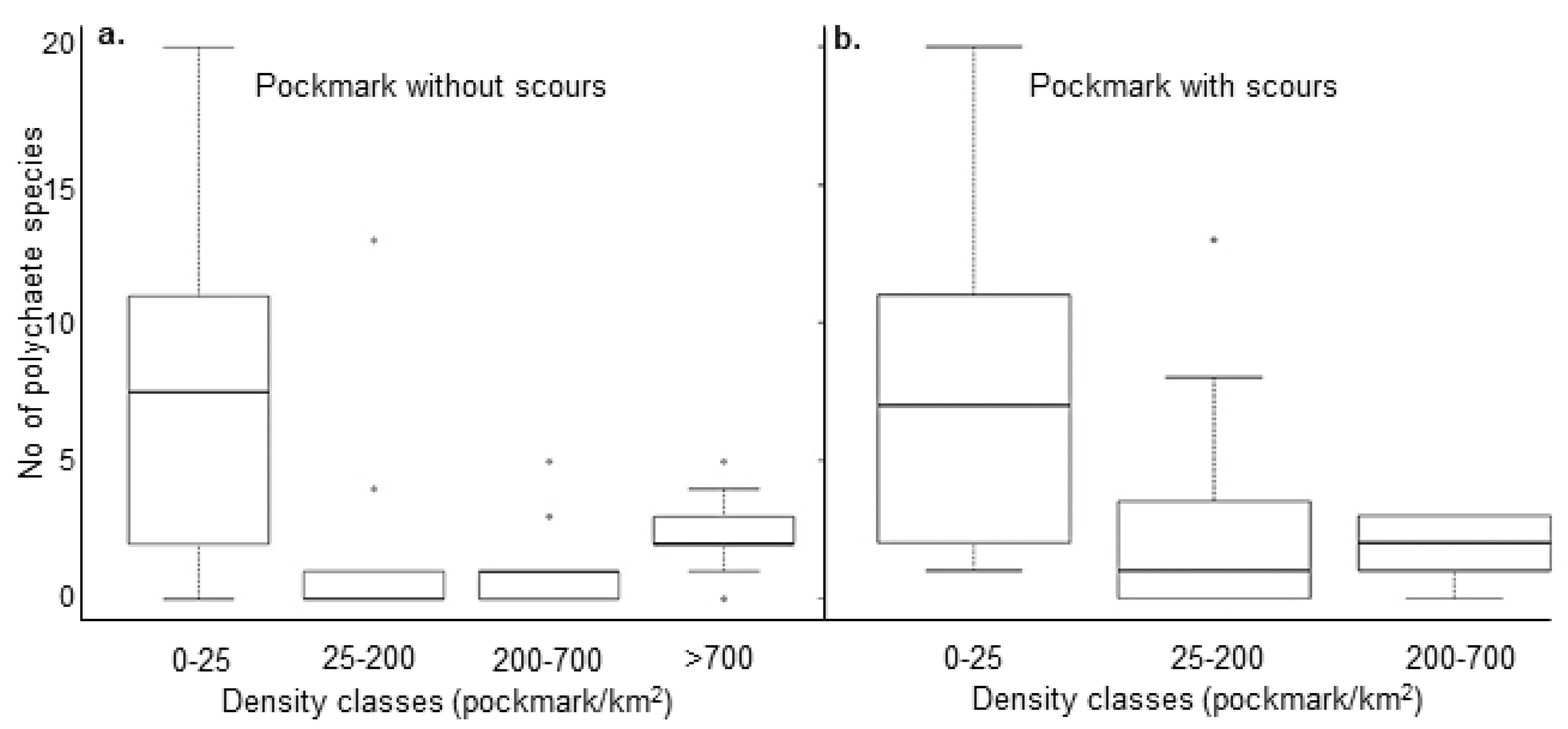
3.2.3. Polychaete Analysis

A total of 38 grab and box core samples were considered for assemblage data. There were three outliers (one for each area) in assemblage data that were identified by their isolation from the main cluster. Statistical analyses were thus performed with and without these (see supplement Figure S5 for details on the distribution). There were no significant differences in polychaete assemblages for pockmark density without scours (including outliers: Pseudo F = 1.2583, p = 0.051; excluding outliers: Pseudo F = 1.1909, p = 0.107). In contrast, there were significant differences in assemblages among pockmark density classes with scours (including outliers: Pseudo F = 1.4036, p = 0.023; excluding outliers: Pseudo F = 1.14548, p = 0.018). Pairwise comparisons revealed significant assemblage (p = 0.005) differences between only the lowest densities classes of scoured pockmarks (<25/km² and 25 to 200/km²).

A total of 51 samples were considered for species richness data. Among pockmark density classes without scours, species richness was significantly different (df = 3, F = 8.7349, p = 0.0001). Tukeys HSD pairwise tests showed significantly more species in the lowest density class (<25 pockmarks/km²) than in the other three higher density classes (Figure 12a). Similarly, species richness was significantly different among pockmark density classes with scours (df = 2, F = 8.6768, p = 0.0006), with more species collected in the lowest density class than the higher density classes (Figure 12b).

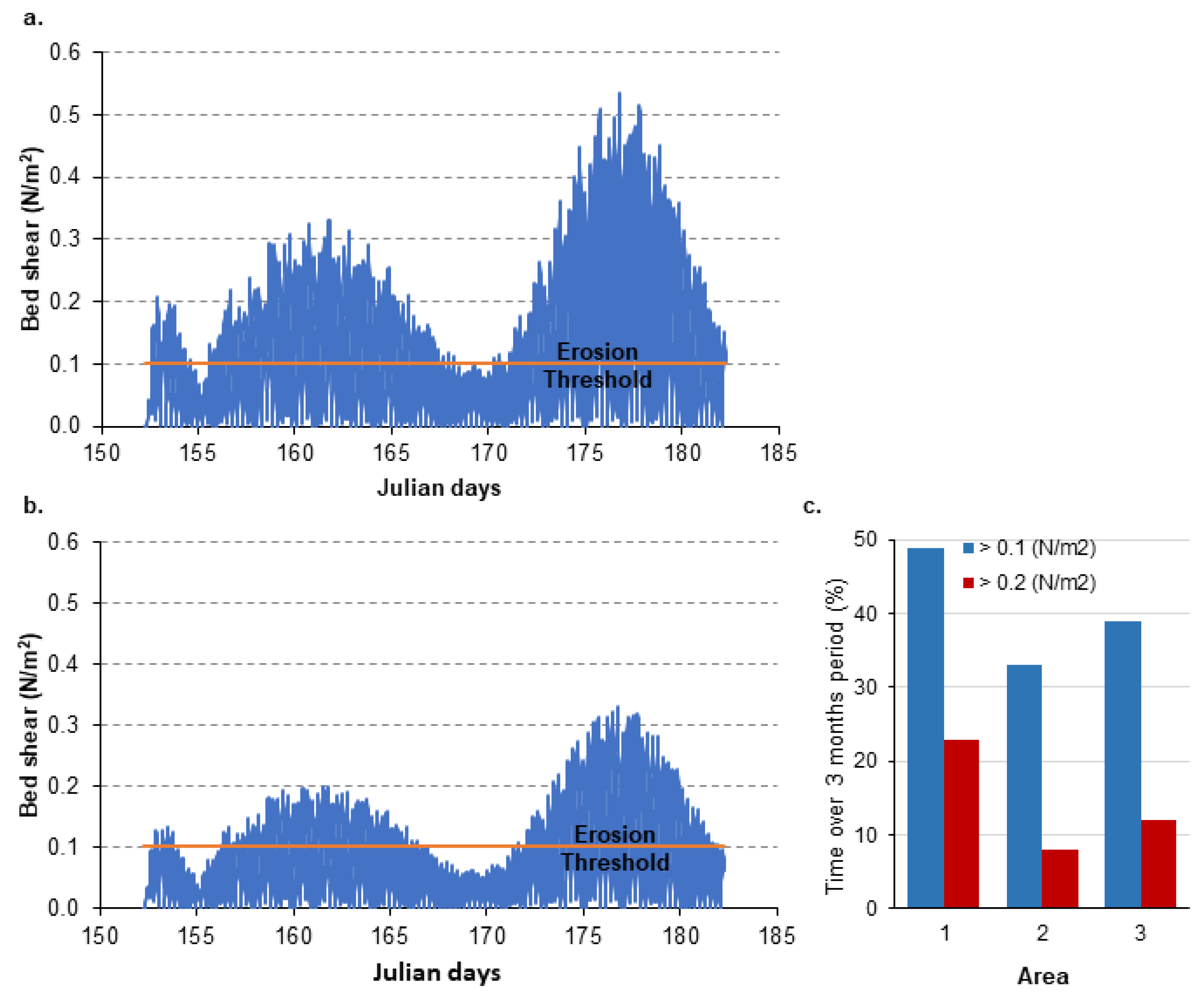
3.2.4. Hydrodynamic Model Analysis

The performance of the model developed here was considered good as the model replicated the growth of the tidal amplitude from the edge of the shelf to the shoreline. The model results were compared to the Timor Sea mooring array, part of the Integrated Marine Observation System (IMOS), that runs to the shelf edge and records a tidal amplitude that grows from plus 3 m at the shelf edge to 6 m on the inner shelf. Results were also correlated with other mooring sites and tide gauges, including Darwin Harbour, Melville and Milner Bay, and inshore the Gulf of Carpentaria.

There is no data available on the bed shear stress erosion threshold for this area above which sediment transport would occur. However, a value of 0.1 N/m² is considered an appropriate value for reasonably cohesive sediments, such as the ones found in this study area [49] Over the three months period modelled for the study area, bed shear stress exceeded 0.1 N/m² for over 33% of the time and 0.2 N/m² for over 8% of the period (Figure 13). Area 1 is exposed to the longest period of bed shear stress exceeding the threshold (49%), while Area 2 the least (12%). Over periods of many years, even the periods of high bed shear stress would be sufficient to provide scour energy on the seabed. Analyses of the modelled current velocities (directions) for all areas suggest a strong bi-directionality with a slight dominance of the current in the NW direction (Figure 14).

4. Discussion

4.1. Confidence Assessment of the Semi-Automated Method

Method GA1 used to identify pockmarks and accompanying scour mark was compared to the BGS combined delineation approach and a second unpublished method developed by Geoscience Australia (GA2). The comparative analysis shows that while all pockmarks in the area were identified within 10% uncertainty and is consistent with other semi-automated methods [10], the BGS method identified 60% more individual pockmarks than GA1. This suggests that there are likely considerably more individual pockmarks in the overall study area, than the 220,508 pockmarks identified. Uncertainties associated with pockmark scour direction, although not quantified here, were considered low due to the large sample number (~40,000; supplementary material). However, for the ‘slice’ of directions associated with bearings having similar bearings to the survey lines (i.e., between 135° and 150°, and its opposite 315° to 330°), this ‘slice’ may be misrepresented because step 4 of GA1 method eliminated these polygons (Figure 5).

Considering that all three methods were developed separately and with different objectives in mind, the results are promising in terms of semi-automatically identifying pockmarks from a range of pockmark fields of varying density (Figure 7). The analysis suggests that while the objective of the study may drive the choice of a preferential method, e.g., scoured pockmarks may be better mapped using a method based on BPI algorithm (GA1), using a combined approach may be ideal to fully characterise any type of pockmarks. Moreover, the comparative analysis provides confidence in using the results of GA1 method over the whole study area to address hypotheses about pockmark formative processes.

4.2. Pockmark Formation and Ecosystem Contribution

Examination of shallow sub-bottom profiles across the survey areas suggests an absence of deeply-sourced gas with no evidence of gas migration from the sub-surface (Figure 2). However, in the sediment samples examined, the concentration of CO₂ in sediment porewater (as TCO₂) is particularly high, approximately twice as high in these sediments compared to elsewhere on the Australian continental shelf (Figure 11). Without evidence for gas sourced from depth, this suggests that the CO₂ is derived from recent (i.e., shallow) sediments, and in turn must imply that organic matter (OM) trapped in the shallow sediment is breaking down rapidly. Our hypothesis for the origin of high pockmark densities in the Oceanic Shoals involves the concept of OM priming (or cometabolism), which pertains to the enhanced remineralisation of refractory sediment-bound OM through the breakdown of more labile OM (see conceptual model in Figure 15) [50]. Carbonate banks in the study area rise tens of meters above soft sediment plain where seabed sediments are often in the euphotic zone (~<60 m) and conditions thus are suitable for the growth of benthic algae as the local source of OM [37]. The shedding of labile organic matter from banks is a contemporary mechanism and likely occurs due to the relatively high current velocities in the region. This is supported by the hydrodynamic current model results (Figure 13 and Figure 14) and the observed scouring of the pockmarks (Figure 3). The lower TOC concentrations per unit surface area of sediment in the high-density pockmark fields may provide evidence for OM priming, on the assumption that some particle bound OM had been mineralised into dissolved CO₂ (Figure 10b). In our conceptual model (Figure 15), the high porewater CO₂ concentrations observed reflect a combination of factors including elevated sedimentary TOC concentrations, the break-down of labile OM shed from the banks, the cometabolism of particle-bound OM and restricted permeability imposed by fine sediments (including the marl-like CaCO₃ content in the mud fraction). Pockmarks could arise if this combination of factors creates saturation with respect to CO₂ followed by gas production.

The data from the Oceanic Shoals region are similar to data from the Petrel Sub-basin (Figure 1) where high TCO₂ in shallow sediments and pockmark formation was attributed to the breakdown of OM and CaCO₃ in the shallow subsurface [29,33]. There, pockmarks are abundant and their distribution correlates strongly with the known distribution of multiple shallowly buried paleochannels, similar to Area 2 here (Figure 2). In the Petrel Sub-basin study, mangrove-derived OM was abundant. Whilst in this study the OM is understood to be sourced from marine biota that inhabit the banks, the co-location and similarity in shape of the high-density field with the cross-shelf valley suggest that OM may also be sourced from the buried paleochannel. Although the OM source generally appears different for the study area (mainly banks), there is a broad similarity in pockmark formation in these two separate seabed regions of the Bonaparte Basin. This hypothesis, in turn, suggests that it likely can be applied elsewhere in this immediate region, including the pockmark fields identified on the Darwin Shelf [24]. It has been suggested that pockmark formation in this region may be due to the presence of banks focusing fluid flow from the shallow sub-surface [29]. The evidence from this study neither supports nor negates the latter hypothesis.

The biogeochemical and physical environment of the pockmark fields appear to drive some of the polychaetes biodiversity in this area. Infauna analysis showed distinct polychaete assemblages and higher richness associated with low density pockmark fields (<25/km). These fields occupy 15% of the study area, are located randomly (Figure 6) and are associated with coarser grain-size (large proportion of shelly sand and gravel texture, as per high % CaCO₃) where TCO₂ concentrations are at their lowest (Figure 15). In some environments, sediment grain size can regulate infaunal communities, with sand content increasing oxygen permeability and associated habitat availability beneath the seafloor surface [51]. However, sediment grain-size is unlikely to be the primary determinant of infaunal species distributions, with other factors such as hydrodynamics, nutrient availability, and biological interactions being key drivers [52]. This is supported by previous analyses of polychaete assemblages in northern Australia in which sediment grain-size was shown to be weakly related to polychaete assemblages and richness [53,54]. Alternatively, as per the intermediate disturbance hypothesis [15], polychaetes may be responding to seabed disturbances associated with active pockmark fields, with successional communities being more prevalent in pockmarks as disturbances such as gas expulsion occur (Figure 15). For example, two groups of pockmarks in the Bay of Fundy were each associated with discrete megafaunal communities, one category supporting pre-equilibrium communities and the other supporting equilibrium communities [53]. Further work is needed on this relationship, including targeted sampling within and outside individual pockmarks.

4.3. Pockmark Maintenance and Contribution to Hydrodynamic Knowledge

Correlation of the observed pockmark scours (Figure 5) with the hydrodynamic model results (Figure 14) suggest that at a regional scale, seabed currents are dominated by the SE-NW tidal flow. Results also indicate that small differences in the predominant modelled and observed directions between each mapped area exist (Figure 5 and Figure 14). Given this strong regional agreement, the fine-scale variations observed within an area can give valuable insight into seabed and oceanographic processes at a scale finer than model resolution (Figure 3 and Figure 7). For example, the scattering of the scour directions observed in Area 1 compared to the more dominant bi-directionality observed in Areas 2 and 3 (Figure 5) suggest that the presence of larger and shallower banks generates more turbulence.

Though the modern seabed within the Bonaparte Basin is in places sediment-starved [21,28], turbulence within pockmarks enhances sediment suspension [11,12]. Given the strong tides here, the presence of open pockmarks within the organic-rich seabed sediments of the Bonaparte shelf suggests that they are active and that there is insufficient sedimentation to bury them faster than they form. Cores collected within the central Bonaparte Basin to the southeast of this study area suggest that post-LGM sediment thickness in the center of the basin is less than few meters [26]. This may explain the small size and depth of the pockmarks with smaller pockmarks typically forming in thinner sedimentary strata [55]. Furthermore, even though high turbidity in the water column was observed [20], the overall bed shear stress is enough to support erosion and mobilisation, while preventing settling of the sediments (Figure 14).

The wide spectrum of shapes exhibited by the pockmarks indicates that they provide an integrated record of the various stages of their formation (Figure 7). It is however, difficult to attribute whether scouring is associated with the formation of the pockmark at a specific time within a tidal cycle or that it reflects a long-term scouring process attributed to the integrated tidal regime. Some studies show that eccentricity of pockmarks is made at the time of the pockmark formation [18] and that it is unlikely that modern currents are reshaping inactive pockmarks, while others suggest that pockmark-scale turbulence plays a role in the excavation and scouring of pockmarks [11,12]. The intermixed variability in the shapes and scour directions observed over a small area here indicates that currents at the time of formation drive the eccentricity of the pockmark, but that scouring is ongoing thereafter.

5. Conclusions

On the northern Australian continental shelf, pockmark formation appears related to the decomposition of organic material which is richly preserved within the shallow sub-surface. Where carbonate banks are the primary point source for organic detritus, pockmarks become concentrated around the banks and are modified by tidal currents that are steered by the banks. As such, the morphometric data extracted here for large numbers of pockmarks provides a robust proxy to support modelling of local to regional hydrodynamics. Local variability in sediment texture and geochemistry around carbonate banks also reflects local organic input and appears to influence polychaetes biodiversity within sediments; but it also relates to seabed disturbance as driven by pockmark formation. In summary, there are multiple interactions that influence pockmark form and distribution. As more pockmarks fields are unveiled by the increased availability of high-resolution seabed data, semi-automated characterisation of pockmarks will become essential and better understanding of the seabed processes will be achieved.

References

1. King, L.H.; MacLean, B. Pockmarks on the Scotian shelf. Geol. Soc. Am. Bull. 1970, 81, 3141–3148. [Google Scholar] [CrossRef]
2. Judd, A.G.; Hovland, M. Seabed Fluid Flow: The Impact on Geology, Biology and the Marine Environment; Cambridge University Press: Cambridge, UK, 2007; p. 475. [Google Scholar]
3. Nicholas, W.A.; Carroll, A.; Picard, K.; Radke, C.L.; Chen, J.; Howard, F.; Siwabessy, J.P.; Dulfer, H.; Tran, M.; Consoli, C.; et al. Seabed Environments, Shallow Sub-Surface Geology and Connectivity, Petrel Sub-Basin, Bonaparte Basin, Timor Sea; Geoscience Australia: Canberra, Australia, 2014; p. 124.
4. Hovland, M.; Gardner, J.V.; Judd, A.G. The significance of pockmarks to understanding fluid flow processes and geohazards. Geofluids 2002, 2, 127–136. [Google Scholar] [CrossRef]
5. Tjelta, T.I.; Svanø, G.; Strout, J.M.; Forsberg, C.F.; Planke, S.; Johansen, H. Gas seepage and pressure build-up at a North Sea platform location: Gas origin, transportation, and potential hazards. In Proceedings of the Offshore Technology Conference (OTC), Houston, TX, USA, 30 April–4 May 2007; p. 11, OTC paper no. 18699. [Google Scholar]
6. Harris, P.T.; Baker, E.K. Seafloor Geomorphology as Benthic Habitat, 1st ed.; Elsevier: London, UK, 2012; p. 900. [Google Scholar]
7. Decker, C.; Olu, K. Does macrofaunal nutrition vary among habitats at the Håkon Mosby mud volcano? Cahiers Biol. Mar. 2010, 51, 361–367. [Google Scholar]
8. Rise, L.; Bellec, V.K.; Chand, S.; Bøe, R. Pockmarks in the southwestern Barents Sea and Finnmark fjords. Nor. J. Geol. Norsk Geol. Foren. 2015, 94, 263–281. [Google Scholar] [CrossRef]
9. Sun, Q.; Wu, S.; Hovland, M.; Luo, P.; Lu, Y.; Qu, T. The morphologies and genesis of mega-pockmarks near the Xisha Uplift, South China Sea. Mar. Petroleum Geol. 2011, 28, 1146–1156. [Google Scholar] [CrossRef]
10. Andrews, B.D.; Brothers, L.L.; Barnhardt, W.A. Automated feature extraction and spatial organization of seafloor pockmarks, Belfast Bay, Maine, USA. Geomorphology 2010, 124, 55–64. [Google Scholar] [CrossRef]
11. Brothers, L.L.; Kelley, J.T.; Belknap, D.F.; Barnhardt, W.A.; Koons, P.O. Pockmarks: Self-scouring seep features? In Proceedings of the 7th International Conference on Gas Hydrates (ICGH 2011), Edinburgh, Scotland, UK, 17–21 July, 2011; p. 10, Paper no. 326. [Google Scholar]
12. Brothers, L.L.; Kelley, J.T.; Belknap, D.F.; Barnhardt, W.A.; Andrews, B.A.; Landon Maynard, M. Over a century of bathymetric observations and shallow sediment characterization in Belfast Bay, Maine USA: Implications for pockmark field longevity. Geo-Mar. Lett. 2011, 31, 237–248. [Google Scholar] [CrossRef]
13. Szpak, M.T.; Monteys, X.; O’Reilly, S.S.; Lilley, M.K.S.; Scott, G.A.; Hart, K.M.; McCarron, S.G.; Kelleher, B.P. Occurrence, characteristics and formation mechanisms of methane generated micro-pockmarks in Dunmanus Bay, Ireland. Cont. Shelf Res. 2015, 103, 45–59. [Google Scholar] [CrossRef]
14. Webb, K.E.; Barnes, D.K.A.; Plankea, S. Pockmarks: Refuges for marine benthic biodiversity. Limnol. Oceanogr. 2009, 54, 1776–1788. [Google Scholar] [CrossRef]
15. Webb, K.E.; Barnes, D.K.A.; Gray, J.S. Benthic ecology of pockmarks in the Inner Oslofjord, Norway. Mar. Ecol. Prog. Ser. 2009, 387, 15–25. [Google Scholar] [CrossRef]
16. Wildish, D.J.; Akagi, H.M.; McKeown, D.L.; Pohle, G.W. Pockmarks influence benthic communities in Passamaquoddy Bay, Bay of Fundy, Canada. Mar. Ecol. Prog. Ser. 2008, 357, 51–66. [Google Scholar] [CrossRef]
17. Przeslawksi, R.; Glasby, C.; Nichol, S. Polychaetes (Annelida) of the Oceanic Shoals region, northern Australia: Considering small macrofauna in marine management. Mar. Freshw. Res. 2018. submitted. [Google Scholar]
18. Gafeira, J.; Long, D.; Diaz-Doce, D. Semi-automated characterisation of seabed pockmarks in the central North Sea. Near Surf. Geophys. 2012, 10, 303–314. [Google Scholar] [CrossRef] [Green Version]
19. Weiss, A.D. Topographic Position and Landforms Analysis. In Proceedings of the ESRI International User Conference, San Diego, CA, USA, 9–13 July 2001. [Google Scholar]
20. Gafeira, J.; Dolan, M.F.J.; Monteys, X. Geomorphometric Characterization of Pockmarks by using a GIS-based Semi-automated Toolbox. Geosciences 2018, 8, 154. [Google Scholar] [CrossRef]
21. Nichol, S.L.; Howard, F.J.F.; Kool, J.; Stowar, M.; Bouchet, P.; Radke, L.; Siwabessy, J.; Przeslawski, R.; Picard, K.; Alvarez de Glasby, B.; et al. Oceanic Shoals Commonwealth Marine Reserve (Timor Sea) Biodiversity Survey: GA0339/SOL5650 Post-Survey Report; Geoscience Australia: Canberra, Australia, 2013; p. 112.
22. Van Andel, T.H.; Veevers, J.J. Morphology and sediments of the Timor Sea. Department of National Development, Bureau of Mineral Resources. Geol. Geophys. Bull. 1967, 83, 186. [Google Scholar]
23. Heap, A.D.; Harris, P.T. Geomorphology of the Australian margin and adjacent seafloor. Aust. J. Earth Sci. 2008, 55, 555–585. [Google Scholar] [CrossRef]
24. Przeslawski, R.; Daniell, J.; Anderson, T.; Barrie, V.; Heap, A.; Hughes, M.; Li, J.; Potter, A.; Radke, L.; Siwabessy, J.; et al. Seabed Habitats and Hazards of the 54 Oceanic Shoals Marine Biodiversity Survey: GA0339/SOL5650—Post Survey Report Joseph Bonaparte Gulf and Timor Sea, Northern Australia; Geoscience Australia Record: Canberra, Australia, 2011; p. 156.
25. Heap, A.D.; Przeslawski, R.; Radke, L.; Trafford, J.; Battershill, C.; Shipboard Party. Seabed Environments of the Eastern Joseph Bonaparte Gulf, Northern Australia: SOL4934 Post Survey Report; Geoscience Australia Record: Canberra, Australia, 2010; p. 81.
26. West, B.G.; Conolly, J.R.; Blevin, J.E.; Miyazaki, S.; Vuckovic, V. Petroleum Prospectivity of the East Malita Graben area, Bonaparte Basin; Bureau of Mineral Resources, Geology and Geophysics Record: Canberra, Australia, 1992. [Google Scholar]
27. Yokoyama, Y.; De Deckker, P.; Lambeck, K.; Johnston, P.; Fifield, L.K. Sea-level at the Last Glacial Maximum: Evidence from northwestern Australia to constrain ice volumes for oxygen isotope stage 2. Palaeogeogr. Palaeoclimatol. Palaeoecol. 2001, 165, 281–297. [Google Scholar] [CrossRef]
28. Yokoyama, Y.; Lambeck, K.; De Deckker, P.; Johnston, P.; Fifield, K. Timing of the Last Glacial Maximum from observed sea-level minima. Nature 2000, 406, 713–716. [Google Scholar] [CrossRef] [PubMed]
29. George, T.; Cauquil, E. A multi-disciplinary site investigation for the assessment of drilling geohazards and environmental impact within the northern Bonaparte Basin. Preview 2010, 148, 41–44. [Google Scholar]
30. Lees, B.G. Recent terrigenous sedimentation in Joseph Bonaparte Gulf, Northwestern Australia. Mar. Geol. 1992, 103, 199–213. [Google Scholar] [CrossRef]
31. Taupp, T.; Hellmann, C.; Gergs, R.; Winkelmann, C.; Wetzel, M.A. Life Under Exceptional Conditions—Isotopic Niches of Benthic Invertebrates in the Estuarine Maximum Turbidity Zone. Estuar. Coasts 2017, 40, 502. [Google Scholar] [CrossRef]
32. Yokoyama, Y.; Purcell, A.; Lambeck, K.; Johnston, P. Shore-line reconstruction around Australia during the Last Glacial Maximum and Late Glacial Stage. Quat. Int. 2001, 83–85, 9–18. [Google Scholar] [CrossRef]
33. Nicholas, W.A.; Nichol, S.L.; Howard, F.J.F.; Picard, K.; Dulfer, H.; Radke, L.C.; Carroll, A.G.; Tran, M.; Siwabessy, P.J.W. Pockmark development in the Petrel Sub-basin, Timor Sea, Northern Australia: Seabed habitat mapping in support of CO2 storage assessments. Cont. Shelf Res. 2014, 83, 129–142. [Google Scholar] [CrossRef]
34. Gunn, P.J. Bonaparte Basin: Evolution and structural framework. In Proceedings of the Petroleum Exploration Society of Australia, Symposium the North West Shelf, Perth, Australia, 10–12 August 1988. [Google Scholar]
35. Bourget, J.; Nanson, R.; Ainsworth, R.B.; Courgeon, S.; Jorry, S.J.; Al-anzi, H. Seismic stratigraphy of a Plio-Quaternary intra-shelf basin (Bonaparte Shelf, NW Australia). In Proceedings of the Petroleum Exploration Society of Australia Symposium, the Sedimentary Basins of Western Australia IV, Perth, Australia, 18–21 August 2013. [Google Scholar]
36. De Deckker, P.; Yokoyama, Y. Micropalaeontological evidence for Late Quaternary sea-level changes in Bonaparte Gulf, Australia. Glob. Planet. Chang. 2009, 66, 85–92. [Google Scholar] [CrossRef]
37. Radke, L.C.; Li, J.; Douglas, G.; Przeslawski, R.; Nicholl, S.; Siwabessy, J.; Huang, Z.; Trafford, J.; Watson, T.; Whiteway, T. Characterising sediments for a tropical sediment-starved shelf using cluster analysis of physical and geochemical variables. Environ. Chem. 2015, 12, 204–226. [Google Scholar] [CrossRef]
38. Gavrilov, A.N.; Siwabessy, P.J.W.; Parnum, I.M. Multibeam Echo Sounder Backscatter Analysis; Centre for Marine Science and Technology: Perth, Australia, 2005. [Google Scholar]
39. Radke, L.; Nicholas, T.; Thompson, P.; Li, J.; Raes, E.; Carey, M.; Atkinson, I.; Huang, Z.; Trafford, J.; Nichol, S. Baseline biogeochemical data from Australia’s continental margin links seabed sediments to water column characteristics. Mar. Freshw. Res. 2017. [Google Scholar] [CrossRef]
40. Evans, J.S.; Oakleaf, J.; Cushman, S.A.; Theobald, D. An ArcGIS Toolbox for Surface Gradient and Geomorphometric Modeling, version 2.0-0. 2014. Available online: http://evansmurphy.wix.com/evansspatial (accessed on 19 March 2018).
41. Fisher, P.; Wood, J.; Cheng, T. Where is Helvellyn? Fuzziness of multi-scale landscape morphometry. Trans. Inst. Br. Geogr. 2004, 29, 106–128. [Google Scholar] [CrossRef]
42. Yokoyama, R.; Shirasawa, M.; Pike, R.J. Visualizing topography by openness: A new application of image processing to digital elevation models. Photogramm. Eng. Remote Sens. 2002, 68, 257–265. [Google Scholar]
43. Clarke, K.R.; Warwick, R.M. Change in Marine Communities: An Approach to Statistical Analysis and Interpretation, 2nd ed.; PRIMER-E: Plymouth, Australia, 2001; p. 172. [Google Scholar]
44. Anderson, M.J.; Gorley, R.N.; Clarke, K.R. PERMANOVAþ for PRIMER: Guide to Software and Statistical Methods; PRIMER-E: Plymouth, UK, 2008. [Google Scholar]
45. Geoscience Australia. The Australian Bathymetry and Topography 2009 250 m. 2009. Available online: http://www.ga.gov.au/metadata-gateway/metadata/record/89581/ (accessed on 19 March 2018).
46. Radke, L.C.; Webber, E. Seafloor Environments of the eastern Timor Sea, Northern Australia: Mineralogy of Seabed Sediments; Geoscience Australia: Canberra, Australia, 2014.
47. Shepard, F.P. Nomenclature based on sand-silt-clay ratios. J. Sediment. Petrol. 1954, 24, 151–158. [Google Scholar]
48. Keil, R.G.; Mayer, L.M.; Quay, P.D.; Richey, J.E.; Hedges, J.I. Loss of organic matter from riverine particles in deltas. Geochim. Cosmochim. Acta 1997, 61, 1507–1511. [Google Scholar] [CrossRef]
49. Van Rijn, L.C. Principles of Sediment Transport in Rivers, Estuaries and Coastal Seas. 1993. Available online: www.aquapublications.nl (accessed on 19 March 2018).
50. Van Nugteran, P.; Moodley, L.; Brummer, G.-J.; Heip, C.H.R.; Herman, P.M.; Middleburg, J.J. Seafloor ecosystem functioning: The importance of organic matter priming. Mar. Biol. 2009, 156, 2277–2287. [Google Scholar] [CrossRef] [PubMed]
51. Snelgrove, P.V.R.; Butman, C.A. Animal-sediment relationships revised: Cause versus effect. Oceanogr. Mar. Biol. Annu. Rev. 1994, 32, 111–177. [Google Scholar]
52. McArthur, M.; Brooke, B.; Przeslawski, R.; Ryan, D.A.; Lucieer, V.; Nichol, S.; McCallum, A.W.; Mellin, C.; Cresswell, I.D.; Radke, L.C. On the use of abiotic surrogates to describe marine benthic biodiversity. Estuar. Coast. Shelf Sci. 2010, 88, 21–32. [Google Scholar] [CrossRef]
53. Przeslawski, R.; McArthur, M.A.; Anderson, T.J. Infaunal biodiversity patterns from Carnarvon Shelf (Ningaloo Reef), Western Australia. Mar. Freshw. Res. 2013, 64, 573–583. [Google Scholar] [CrossRef]
54. Connell, J.H. Diversity in tropical rain forests and coral reefs. Science 1978, 199, 1302–1310. [Google Scholar] [CrossRef] [PubMed]
55. Brothers, L.L.; Kelley, J.T.; Belknap, D.F.; Barnhardt, W.A.; Andrews, B.D.; Legere, C.; Hughes Clarke, J.E. Shallow stratigraphic control on pockmark distribution in north temperate estuaries. Mar. Geol. 2012, 329–331, 34–45. [Google Scholar] [CrossRef]
Figure 1. Location map showing the study area (Oceanic Shoals survey) within the Oceanic Shoals Australian Marine Park (brown outline) in the Timor Sea, Northern Australia. Geological setting is also included with the encompassing Bonaparte Basin as a bold dashed line and its subdivisions as continuous line. Post-survey reports that are associated with the survey outlined in this figure are as followed: Oceanic Shoals [21], Petrel Sub-basin [29], LaPerouse-Durville [29], Darwin Shelf [24,25], cores [27]. Figure modified from [21]
Geosciences 08 00195 g001
Figure 2. Hillshaded bathymetry data of the three survey areas in the Oceanic Shoals Australian Marine Park (AMP) and location of sediment samples used for the various analyses. (a) Area 1, (b) Area 2 overlaid on the 250 m bathymetry grid [38] and showing the area in relation to the cross-shelf valley existing within the Sahul Syncline, and (c) Area 3 also showing the location of Figure 7. (d) Sub-bottom profile across Area 2 cross-shelf valley (b).
Geosciences 08 00195 g002
Figure 3. (a) Geomorphic map of Area 1. (b) Hillshaded backscatter inset showing scoured pockmarks with high backscatter intensity centers (red). (c) Bank profiles taken along the narrow axis of all banks in the study area. Colours are associated with the area in which the bank was profiled.
Geosciences 08 00195 g003
Figure 4. Summary steps involved in the extraction and characterisation of pockmarks. See supplementary material for details.
Geosciences 08 00195 g004
Figure 5. Rose diagrams of observed scour direction for each of the area analyzed. (a) Area 1; (b) Area 2; (c) Area 3; and (d) combined areas.
Geosciences 08 00195 g005
Figure 6. Density distribution of pockmark without scour (to; blue shades) and with scours (bottom; green shades) within the three survey areas ((a) Area 1, (b) Area 2, and (c) Area 3). The location of the sub-bottom profile presented in Figure 2d is also displayed on b. to indicate the location of the buried paleochannel within the cross-shelf valley of Area 2.
Geosciences 08 00195 g006
Figure 7. Examination of pockmarks identified using the three methods: GA1 (red), British Geological Survey (BGS) (yellow), GA2 (blue). Panels (ad) show the picks using the various methods for the entire test area, while panels (eh) show an inset of the test area in order to present more details. (i) Histogram comparing the total pockmark count (grey bars) and coverage area (coloured bars) between the three automated methods used to identify pockmarks.
Geosciences 08 00195 g007
Figure 8. Ternary diagram illustrating the relative proportions of Sand, Silt, and Clay (after [47]) indicating the dominance of silt over clays in the muddy sediments of the Oceanic Shoals.
Geosciences 08 00195 g008
Figure 9. Sediment characteristics (box plots) and averaged seabed backscatter strength (coloured symbols) for each non-scoured pockmark field density class per area. Similar results were observed for the scoured pockmark.
Geosciences 08 00195 g009
Figure 10. (a) Total organic carbon content (%) of the samples collected in the study area compared to other samples collected on the Australian Shelf highlighting the high Total Organic Carbon (TOC) concentrations at a given grain-size. The data shown here is from samples collected from the 0–2 cm sediment horizon during surveys in the period from October 2007 to May 2013 (see Table 1 in [39]). (b) TOC versus specific surface area of sediments highlighting that sediments from the dense pockmark fields have less TOC per square of sediment than sediments from the low-density pockmark fields.
Geosciences 08 00195 g010
Figure 11. Total carbon dioxide porewater pool concentration (0–2 cm) versus porosity (0–2cm) of the samples collected on the Australian Shelf between October 2007 to May 2013 (see Table 1 in [39] for survey details). The yellow triangles pertain to pockmarked sediment in the Oceanic Shoals AMP survey areas.
Geosciences 08 00195 g011
Figure 12. Boxplots of polychaete species richness among pockmark density classes (a) without scours and (b) with scours.
Geosciences 08 00195 g012
Figure 13. Modelled bed shear stress results for the three months period in (a) Area 1 and (b) Area 3. (c) Comparison of the percent time in the three months modelled period where the bed shear stress exceeded the erosion threshold of 0.1 N/m2 considered for the type of sediments found in the study area [49] and 0.2 N/m2.
Geosciences 08 00195 g013
Figure 14. Near seabed velocities showing the directionality of current for Area 3. Trends for Areas 1 (blue) and 2 (red), as well as the summary trend (yellow) for all the observed data (scours) are also plotted. Note the dominant direction indicated is towards the bearing value indicated.
Geosciences 08 00195 g014
Figure 15. Conceptual model summarising the hypothesis about the formative processes of the pockmark fields in the study area. (a) Overview of the bank-plain system; (b) Low pockmark density scenario where more elevated sand content results in lower porosity compared to finer grain-sizes (shown here as clay and silt particles) and presumably higher permeability (interconnected pore space). Therefore, when OM is mineralised into DIC it does not build up to saturation levels for CO2. Polychaete biodiversity is relatively high because of the increase gas exchange (O2) and more stable conditions. (c) Medium pockmark density scenario where porosity is higher than (a). Permeability may become occluded within sediment micro-niches due to the occurrence of fine sediments (silt and clays) and the swelling of smectite. Limited pockmark formation occurs due to gas build up. Polychaete biodiversity is likely low due to the low O2 concentrations and increasing CO2 concentrations caused by restriction in permeability and the physical disruption to the sediments due to pockmark formation. (d) High pockmark density scenario in which sediments contain more silts and clays creating more micro-niches for gas formation. The gas is expulsed and the seafloor becomes “rugged”. Clay particles have less sediment-bound OM due to OM priming. Sediments are mobilised from pockmarks due to strong near-seabed currents. Low polychaetes biodiversity is presumably due to physical disturbance.
Geosciences 08 00195 g015