Impact of Groundtrack Pattern of a Single Pair Mission on the Gravity Recovery Quality


1
Faculty of Civil Engineering and Transportation, University of Isfahan, Isfahan 81746-73441, Iran
2
Institute of Geodesy, University of Hanover, Schneiderberg 50, 30167 Hannover, Germany
3
Institute of Geodesy, University of Stuttgart, Geschwister-Scholl-Str. 24D, 70174 Stuttgart, Germany
*
Author to whom correspondence should be addressed.
Geosciences 2018, 8(9), 315; https://doi.org/10.3390/geosciences8090315
Submission received: 11 July 2018
/
Revised: 14 August 2018
/
Accepted: 18 August 2018
/
Published: 23 August 2018
(This article belongs to the Special Issue Gravity Field Determination and Its Temporal Variation)
Abstract
:For future gravity satellite missions, aliasing of high frequency geophysical signals into the lower frequencies is one of the most challenging obstacles to recovering true gravity signals, i.e., to recover the truth. Several studies have investigated the impact of satellite groundtrack pattern on the quality of gravity recovery. Among those works, the concept of sub-cycle has been discussed as well. However, most of that research has focused on the impact of sampling patterns on global solutions up to a fixed maximum spherical harmonic coefficient, rather than the associated coefficient defined by the Colombo-Nyquist and modified Colombo-Nyquist rules. This work tries to look more closely into the influence of sampling patterns on the gravity recovery quality for global and regional studies when the Colombo-Nyquist and modified Colombo-Nyquist rules apply. For the regional study, the impact of groundtrack patterns of different satellite constellation scenarios are investigated for a hydrological basin in central Africa. The quality of the gravity products are assessed by different metrics, e.g., by spatial covariance representation. The potential meaning of the sub-cycle concept in terms of global and local impacts is also investigated by different repeat-orbit scenarios with even and odd parities. Different solution scenarios in terms of the original and modified Colombo-Nyquist rules will be discussed. The results of our study emphasize the impact of maximum harmonics of the recovery, the influence of sub-cycle on the local gravity recovery and the mission formation impact on the recovery error.
1. Introduction
Since the launch of the Gravity Recovery and Climate Experiment (GRACE) mission, several research works, e.g., [1,2,3,4,5,6,7,8,9,10,11,12,13] have investigated the performance of next generation satellite gravity missions. Inline (GRACE-like), alternative (advanced) formations (e.g., Pendulum, Cartwheel, LISA), as well as double-pair mission scenarios (two pairs of inline formation) have been studied.
Furthermore, the European Space Agency (ESA) projects “Assessment of a Next Generation Mission for Monitoring the Variations of Earth’s Gravity” [14] and “Assessment of Satellite Constellations for Monitoring the Variations in Earth’s Gravity Field” [15] investigated the science requirements, performance criteria and design of future satellite gravity missions. These two ESA studies briefly discussed two advanced formations and Bender configurations. However, because of the complexity of the technical implementation of alternative formations such as Pendulum, Cartwheel and LISA, their employment as a future gravity mission is currently not of interest to the community [11], although the future technical improvements may bring them back to the consideration.
Some of the aforementioned studies also suggested a range of parameter choices for double-pair satellite missions for full repeat period and sub-Nyquist solutions.
Most of the aforementioned works chose individual constellation scenarios by rough assessments of the sampling behavior of the missions. However, the studies by [5,6,8,15] investigated some performance criteria for their optimal double-pair mission scenario search strategies.
In gravity satellite missions, two sampling descriptions exist, which dictate the quality of the gravity recovery change in space and time domains. First, a Heisenberg-like uncertainty theorem in satellite geodesy addresses the trade-off between spatial and temporal resolution by
i.e., the product of spatial resolution
and the time resolution is constant and equal to with as the revolution time [8,16,17]. Second, the Colombo-Nyquist rule (CNR) requires
where is the number of satellite revolutions within a repeat period in nodal days (α). The formulation means that the number of satellite revolutions in a repeat period should be equal to or larger than twice the maximum spherical harmonic degree () or order () to be detected [18,19]. Indeed, this rule limits the spatial resolution of the gravity recovery. However, the works by [20,21] argue that the spatial resolution can be improved, not by twice the maximum degree or order or , but by a smaller degree or order values. In particular, the work by [21] discusses that those values can even reach or themselves, depending on the parity of the satellite repeat orbit. However, the description by [21] is not fully applicable, and requires further investigations. In fact, this study states that a recoverable gravity solution in a full repeat period can be achieved by the new modified rule when is odd for the near-polar orbits. Later, [8] took the benefit of the proposed modified Colombo-Nyquist rule (MCNR) to achieve sub-Nyquist gravity recovery, although it should be mentioned that the term “sub-Nyquist” in that work is not defined according to sampling distribution and groundtrack pattern evolution, but by fixed values defined by mission revolutions per nodal days. Therefore, in that context, one can consider Nyquist as the upper limit in sampling theorem.
The short-time intervals solutions, called sub-Nyquist solutions, in consequence, may benefit from higher temporal resolution, and thus, less temporal aliasing, compared to the longer span solutions, e.g., defined by CNR. An important benefit of having those solutions is that they can also be employed as de-aliasing products when time-variable gravity solutions of longer time intervals are targeted [22].
Besides the two aforementioned rules, the spatio-temporal groundtrack pattern distribution of a satellite mission scenario can significantly affect the quality of the gravity recovery. Therefore, studying the gap evolution of the satellite mission groundtrack is of a great interest as well. Some studies like [8,12,13,14] investigate the impact of sampling evolution on the gravity recovery quality. For example, [8,14] look into different categories of orbits where drifting, slow skipping and fast skipping orbits, and their impacts on the quality of gravity solutions for single-pair satellite missions are discussed. Moreover, the work by [12] studies the refinement of Colombo-Nyquist and modified Colombo-Nyquist rules for different latitudes rather than at the equator, where the former studies have focused. The paper by [13], on the other hand, looks into the groundtrack pattern evolution of double pair missions where the influence of relative difference of the right ascension of ascending nodes between the two pairs (∆Ω) is investigated. In fact, the paper discusses three reasons for the quality variations of the gravity solutions: (i) the sampling pattern of each satellite pair of a double pair mission with different repeat periods evolves differently in the time domain. (Hence, one should expect that within a specific time-interval gravity solution, e.g., 10-day solution, the groundtrack pattern also changes). (ii) the time-variation of ∆Ω can be responsible for the pattern change which, in turn, influences the quality of the gravity recovery. (That is because the two orbits with different inclination angles have different drifting rates of ∆Ω), and (iii) the gravity signals on the Earth are themselves time-variable and cause quality variations of the solutions within the time.
Besides studying the aforementioned concepts which were briefly discussed, several research works examine the sub-cycle concept. For example, the works by [8,14,15] discuss the meaning of sub-cycle in terms of homogeneity of gap evolution for single pair mission scenarios. The works investigate the impact of the groundtrack pattern and sub-cycle concept on the global gravity recovery up to a fixed spherical harmonic coefficient degree where a big difference between the quality of gravity solutions of drifting and skipping orbits are observed. However, the study by [8] shows that the sub-cycle has no significant meaning in terms of global recovery for a fixed spherical harmonic degree to be solved.
Obviously, it makes more sense if the impact of groundtrack pattern and its time evolution, as well as the sub-cycle concept, are investigated for maximum spherical harmonic degrees by Colombo-Nyquist rule (CNR) and modified Colombo-Nyquist rule (MCNR). In this way, for Low Earth Orbit (LEO) missions, adding a day to the time span of the recovery means adding approximately 8 and 16 degrees and orders to the maximum spherical harmonic coefficient to be solved, respectively, for CNR and MCNR, but as long as the number of nodal days is still smaller than or equal to the full repeat period. Moreover, it might be of interest to observe the impact of even and odd orbit parities () on gravity solutions which are shorter than the full repeat cycle of the mission orbit scenario. The impact of groundtrack pattern on the regional gravity field (i.e., gravity retrieval for a specific region out of the global recovery) where the pattern is denser or when the sub-cycle happens is also worthy of further study. This paper, therefore, addresses the aforementioned research issues. We try to provide a few examples for different scenarios, and discuss potential future work in this research field.
In order to have a clearer overall view of this paper, it is important to mention that the GRACE Follow-on (GFO) mission has already been realized; therefore, the result of this research does not directly address the performance of GFO in the course of its orbit. However, our study tries to address the general impact of the sampling pattern on gravity recovery, which is also of great importance for understanding the quality variations by GFO products in its future life, as it is expected that by different sampling (ground-track pattern change) within GFO at different time-interval solutions, its recovery quality is also going to vary significantly.
Another important point to be mentioned is that, similar to the GRACE mission in the recent years, the science community expects to have short-interval gravity recovery (shorter than month) for GFO as well, particularly since GFO is benefiting from more advanced instrumentation, and hence, fewer measurement errors. That makes the weekly and shorter than weekly solutions more interesting which can be allowed by CNR and partially MCNR, and is the focus of this paper. For this purpose and to investigate the sampling impact on the recovery quality, a few examples are chosen for our study’s scope. Here, we test some scenarios with different “right ascension of ascending node” (RAAN) values over a hydrological basin in central Africa. Indeed, in both theory and reality, RAAN changes with time, and unless implementing mission control by humans during the satellite lifetime (which is rare, and mainly for altitude and repeat-orbit correction), the satellite path is not continuously corrected in order to bring RAAN to its initial value. Therefore, the selected RAAN values and the choice of central Africa in this research work should be seen as examples to study the recovery quality variations in different sampling scenarios. In fact, in this study, we do not address orbit optimization in specifics (which is the function of many other parameters), but instead, we try to address the importance of sampling pattern on the quality of gravity recovery through few examples. The choice of central Africa in the paper refers to its location close to the equator, which means a bigger area on the Earth, and so less dense sampling in the spatial domain when compared with sampling the higher latitudes. This choice can therefore address the sampling impact in a clearer way. Furthermore, the particular choice of the RAAN values refers to different sampling behavior, i.e., to the case where sub-cycle happens and to the cases where it does not happen in that area (and at that specific time).
2. Simulation Environment
2.1. RST Gravity Recovery Simulation Software
For the gravity recovery simulation, a nominal circular orbit simulation package of so-called Reduced-Scale Tool, (RST) (previously called Quick-look Tool, QLT [8,17]) is employed. The software assumes that the satellite orbits are nominal, i.e., the only perturbing force is J2 effect by the Earth flattening, hence the semi-major axis, inclination angle and eccentricity of the satellites are not time-variable parameters [8]. The observation equation is built up by
where is range, is range rate and is range acceleration. is the relative velocity vector and is the unit vector of the inter-satellite distance of the satellite pair. The potential gradient at the first and second satellite positions for the epoch t are and , respectively.
By the RST software, the right side of the equation above is calculated at the nominal positions of the satellites for the time interval of interest. The time-variable potential of the Earth at the positions of the satellites is calculated by the provided time-variable gravity field models at those epochs. Afterwards, the calculated values for the right side of the equation are set to the left side as the observables at those epochs, and the gravitational potential, in terms of spherical harmonics coefficients, is estimated through the system of equations for that time interval. It is important to mention that although the assumption of keeping the satellites in a perfect nominal orbit is not realistic, the simulation software provides a quick comparison of gravity recovery solutions in different mission scenarios, which can later be studied in more details by full-scale recovery tools. An evaluation of the RST has been made with the ll-SST acceleration approach applied to orbits from real orbit integration by [8], which shows a good agreement between the results of the two approaches for gravity recoveries, despite the differences between the two methods.
The equatorial bulge of the Earth (the Earth flattening effect) is responsible for change of the Keplerian elements (argument of perigee rate), (rate of right ascension of the ascending node) and (mean anomaly rate). For circular orbits, the argument of perigee is not defined, but the other two elements change with the following rates:
where a, e and I are respectively the semi-major axis, eccentricity (here sets to zero for the circular orbits) and inclination angle. The parameter stands for the mean motion of the satellite and is the disturbing potential field.
2.2. Geophysical Input Models
For the simulation environment of this study, we employ the dominant mass variations of hydrology, ice and solid Earth of the Earth system by use of the time-variable gravity field models generated within the ESA-project “ESA Earth System Model for Gravity Mission Simulation Studies” [23] as an update to previous ESA models by [24], provided as spherical harmonic coefficients up to degree and order 180 at 6 h intervals. The time-span applied in our study starts from 1 January 1996 for 3-days to 9-days gravity recovery. The difference between two ocean tide models EOT08a [25] and [26], is assumed as the ocean tide error in simulation, where the error is an important source for aliasing of the high frequency signals to the low frequency signals [27]. Moreover, the atmosphere-ocean error (AO error) product from IAPG (TU Munich) is employed for the forward modeling [15]. The AO error model is defined as two atmosphere models difference (ECMWF-NCEP) plus 10% of the ocean signal of the model OMCT. Furthermore, all geophysical forward models are smoothed by Gaussian filter of radius 4000/2Lmax km to avoid ringing effects (Gibbs phenomenon) caused by the truncation error.
2.3. Gap Evolution and the Sub-Cycle Concept
In [14], the sub-cycle concept is defined as follows:
Assuming as the number of orbit revolutions per day, the “Fundamental Interval” gives the angular space between two Ascending Node Crossing (ANX) consecutive in time
The sub-interval is the sampling angle after an entire repeat period (RC)
Therefore, one can rewrite the parameter as follows
The parameter can also be written as
where is the integer part of .
Within , the ANX of days and are always separated by a distance of or sub-intervals .
Two types of orbits can be recognized: (i) drifting orbits when or , and (ii) skipping orbits in the other cases. In a drifting orbit, the sampling of the fundamental interval is very progressive with large unobserved gaps, while a skipping orbit, on the other hand, has a more complex coverage pattern, reducing the persistence of the large unobserved gaps quite fast. In fact, the skipping orbit owns a very wide range of spatial and temporal coverage patterns.
The concept “sub-cycle” (sc) can be defined as the smallest number of days after which an Ascending Node Crossing (ANX) falls at or from the first ANX. According to this definition, the sub-cycle of a drifting orbit is one day. The sub-cycle can be an interesting parameter to measure how fast an orbit is in reducing the largest unobserved gap [8]. Among different kinds of skipping orbits, some orbits also feature one or more pseudo sub-cycle (psc) which can also be an interesting concept to study the temporal sampling of a satellite scenario [14]. The reader is referred to [8,14] for more details about different categories of orbits and the sub-cycle concept with the gap evolution graphs.
3. Results
We simulate different inline (GRACE-like) mission scenarios (Table 1). The scenarios are taken from [8] which try to cover a range of orbits from drifting to fast-skipping with altitudes around 260 to 360 km. The simulations are based on a simplified version of the ll-SST acceleration approach using nominal orbits and the Hill equations [28]. The input models are the relevant time-variable gravity fields of hydrology, ice and solid Earth (HIS) and the difference of two ocean tide models as well as a model for Atmosphere-Ocean (AO) error (see Section 2). The sampling interval of the measurements is . The error is represented as the difference between the gravity recovery (output) and the mean of the HIS time-variable gravity models (input) of the simulations for the same time duration. In all the simulations, the coefficients , , , and are neglected, since the ll-SST measurement concepts for these coefficients are poorly sensitive (although depends on the recovery approach). A white noise model of tracking laser interferometer on the level of range acceleration with a PSD (power spectral density) of is applied in our RST simulation software.
3.1. Global Gravity Recovery Solutions
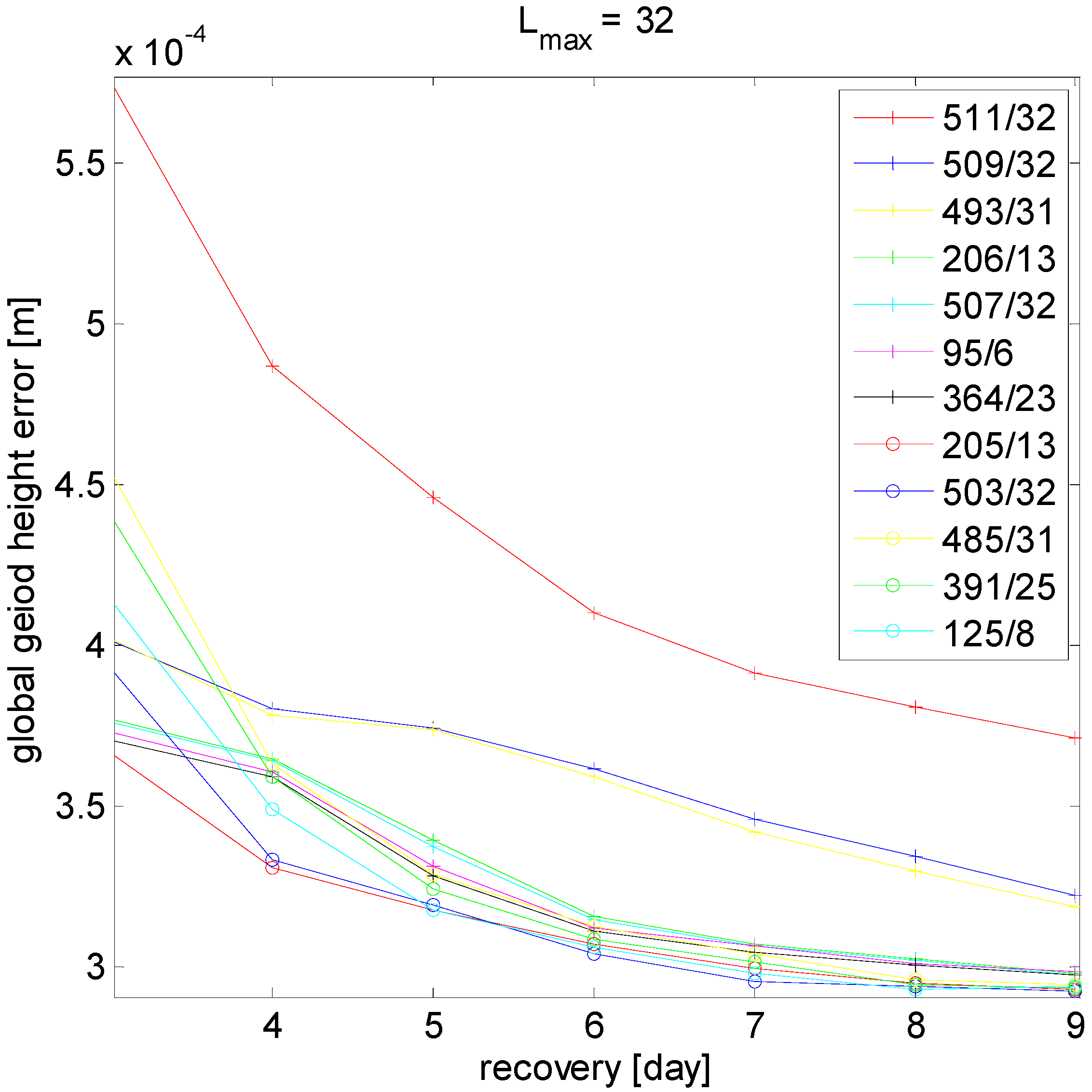
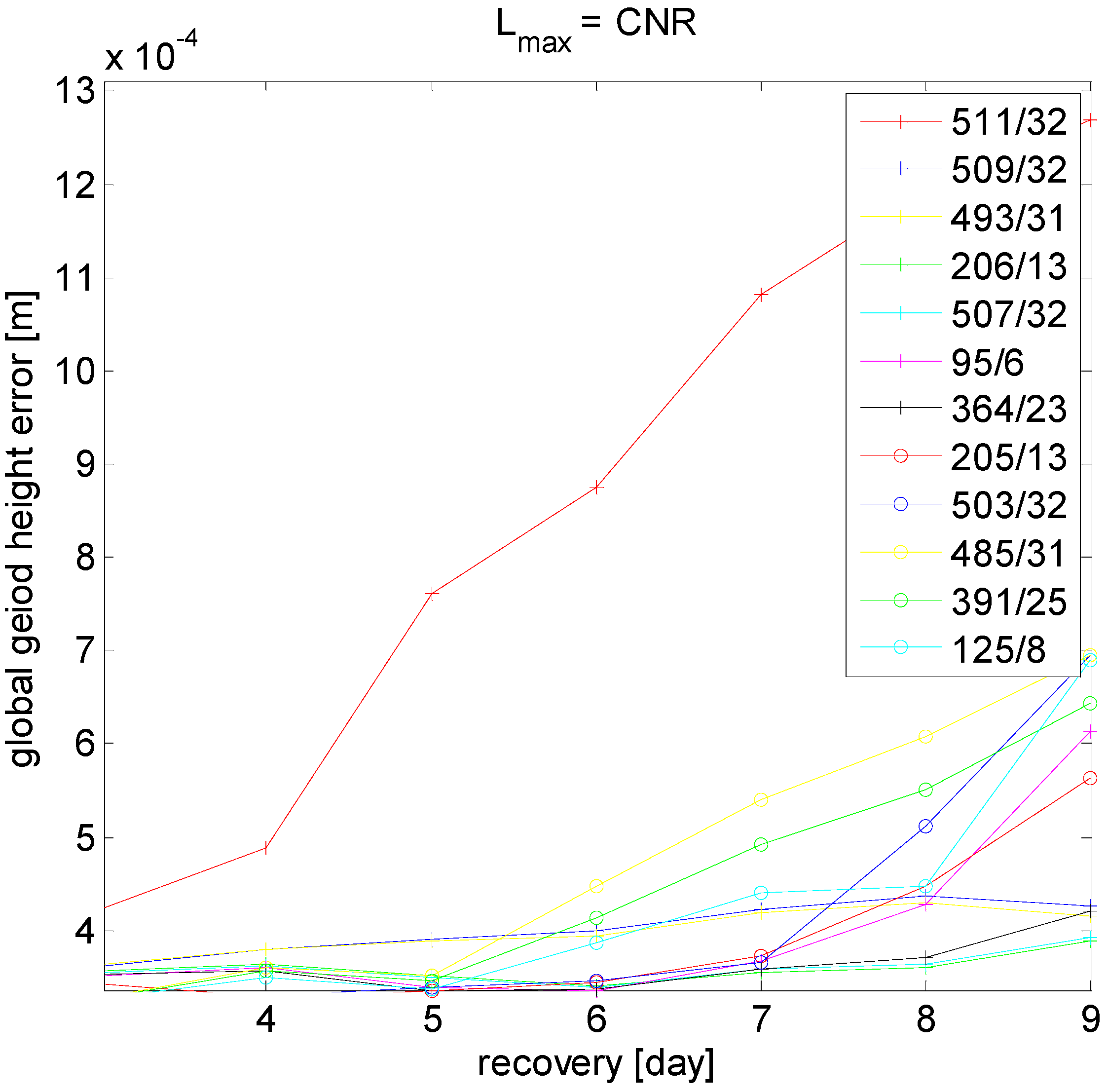
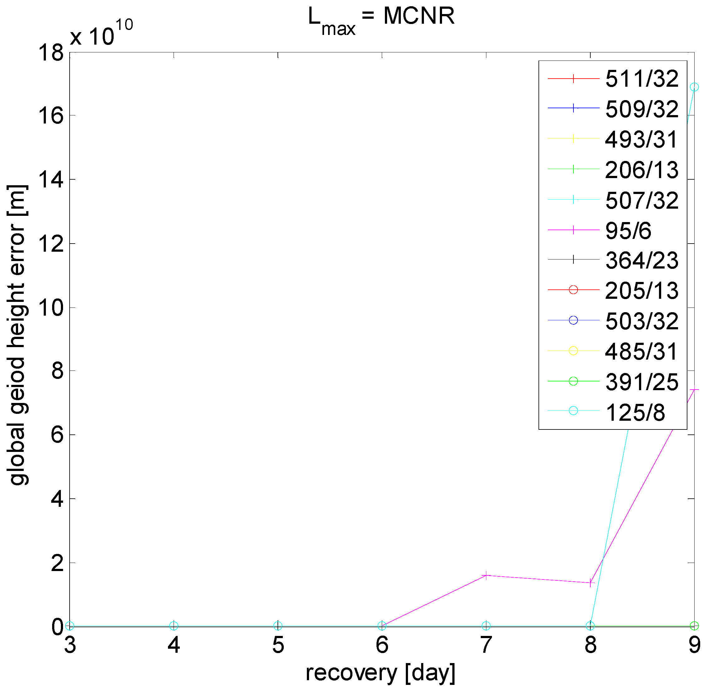
The global Root Mean Square (RMS) error of the mission scenarios of Table 1 are illustrated in Figure 1, Figure 2, Figure 3, Figure 4, Figure 5 and Figure 6 for different recovery cases Lmax = 32, 64, CNR and MCNR. The choices of Lmax = 32, 64 are arbitrary, but selected as two values below CNR (Lmax = 32) and between CNR and MCNR (Lmax = 64) for 6-day solutions (see the next sections). The error is calculated in terms of geoid height for 3-day to 9-day gravity solutions by each mission scenario. As the figures show, the scenario 1 with long full repeat cycle (32 days), but shortest sub-cycle span (1 day), performs the worst. For the MCNR recovery, however, the last scenario (scenario 12) with 8 days repeat cycle, generates extremely large errors on the 8th day. That is clearly not expected, since 8 days is the full repeat cycle of this scenario; therefore, one expects the best performance from the sampling viewpoint for that time-span. The potential reason for such a big error may come from high spatial aliasing of the solution (8-day recovery corresponds to Lmax = 128 for MCNR) and the geometry of the orbit (short full-repeat cycle scenario).
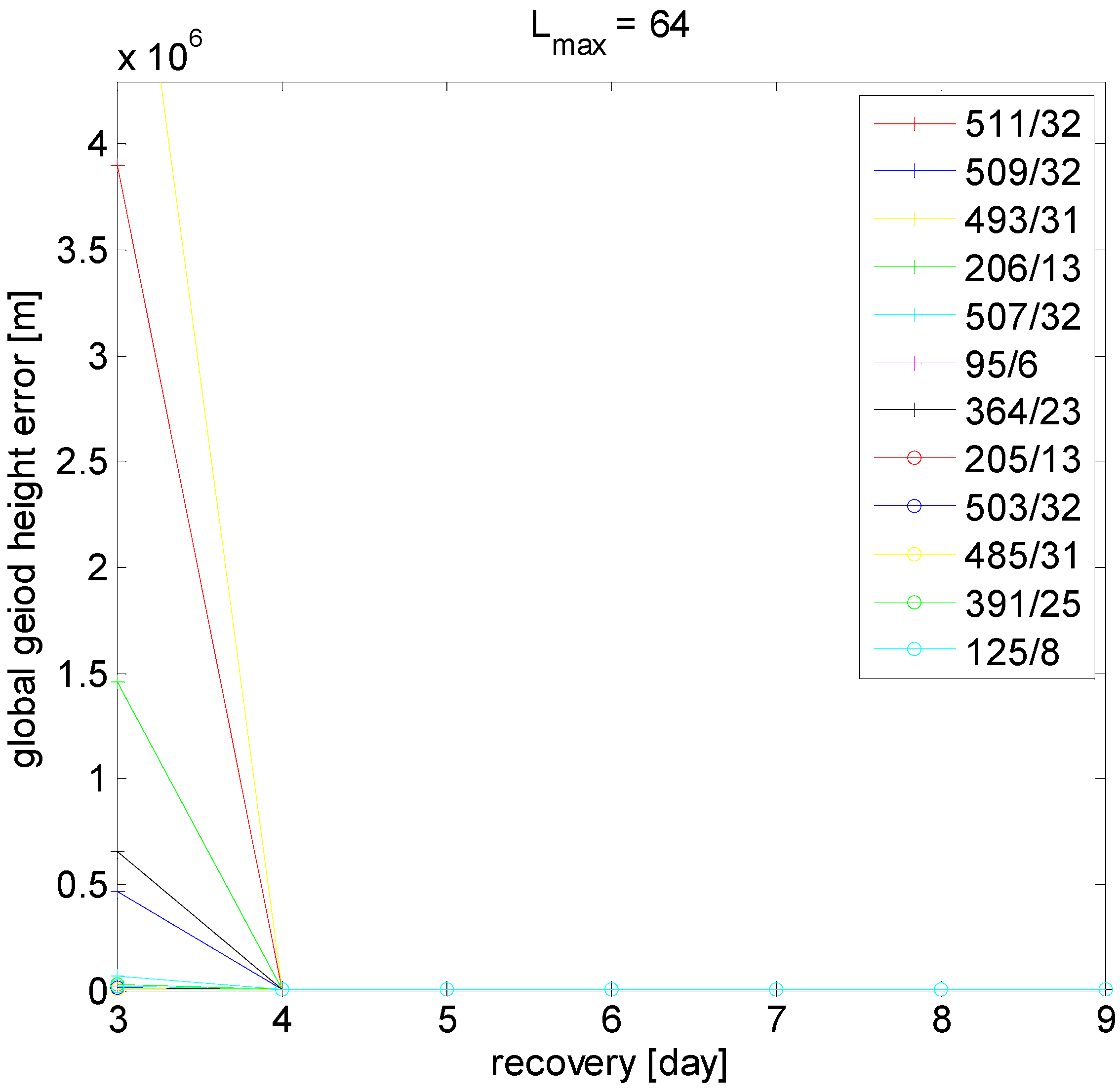
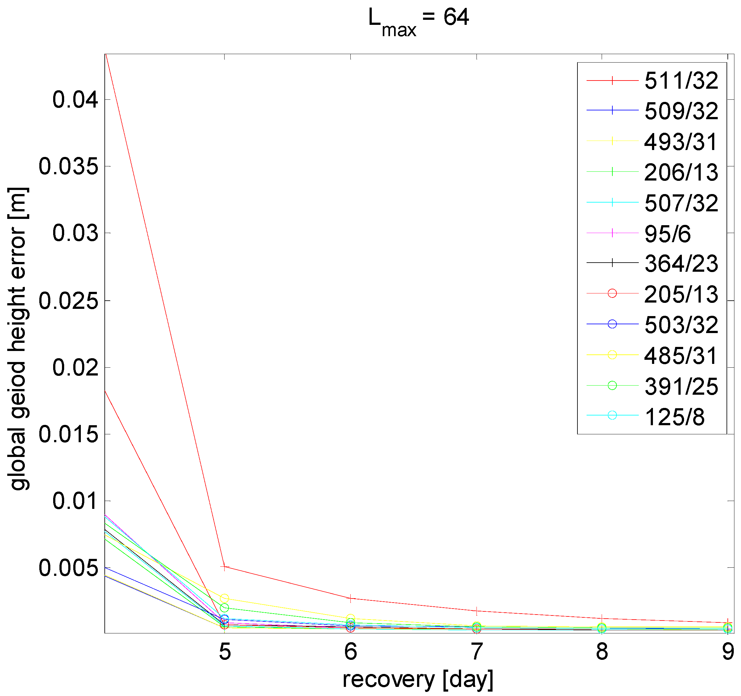
For the case Lmax = 32 (Figure 1), with the increase of the time-pan of the solutions, the recovery error decreases. That is caused by more sampling in space, and therefore, less spatial aliasing, even though the temporal aliasing gradually increases, but not significantly. The same reason also applies for the case Lmax = 64 (Figure 2 and Figure 3). Figure 2, however, shows extremely high errors for solutions shorter than 4 days. In fact, the error is caused by poor conditioning of the normal matrices (singularity problem). The figure is deliberately brought to show that beyond MCNR (here spherical harmonic, SH, degree 48 for 3-day solutions), the recovery is very poor which is, in particular, the case for some orbit configurations.
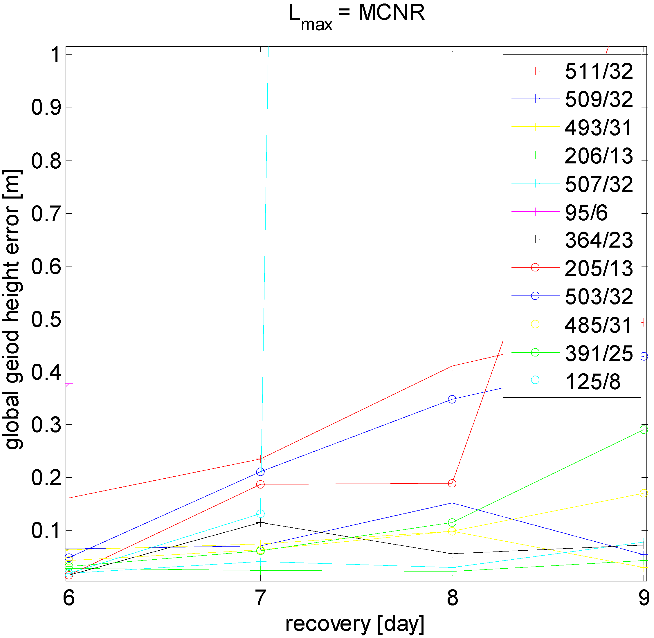
For Lmax = CNR and MCNR, however, it is generally different, i.e., for most of the scenarios, the longer the recovery time-interval, the bigger the error (see Figure 4, Figure 5 and Figure 6). However, different scenarios perform differently. For some scenarios of the case Lmax = CNR, the error increase is significant. The reason for the increase should be associated with the spatial aliasing (by higher spherical harmonic coefficient degree and order to be solved), which is more predominant for some mission scenarios, most likely caused by the geometry of their orbits, and hence, the time evolution of their groundtracks. A similar statement is also valid for the case MCNR (Figure 5 and Figure 6), although more fluctuations are seen in the recovery error of few scenarios. In particular, Figure 5 illustrates very large errors for some orbit scenarios. We think that these extreme error values are caused by severe spatial aliasing through orbit geometry of specific drifting orbit scenario 6 and orbit scenario 12 with short full repeat-cycle of 8 days, even though MCNR is kept.
3.1.1. Two Scenarios for Comparisons
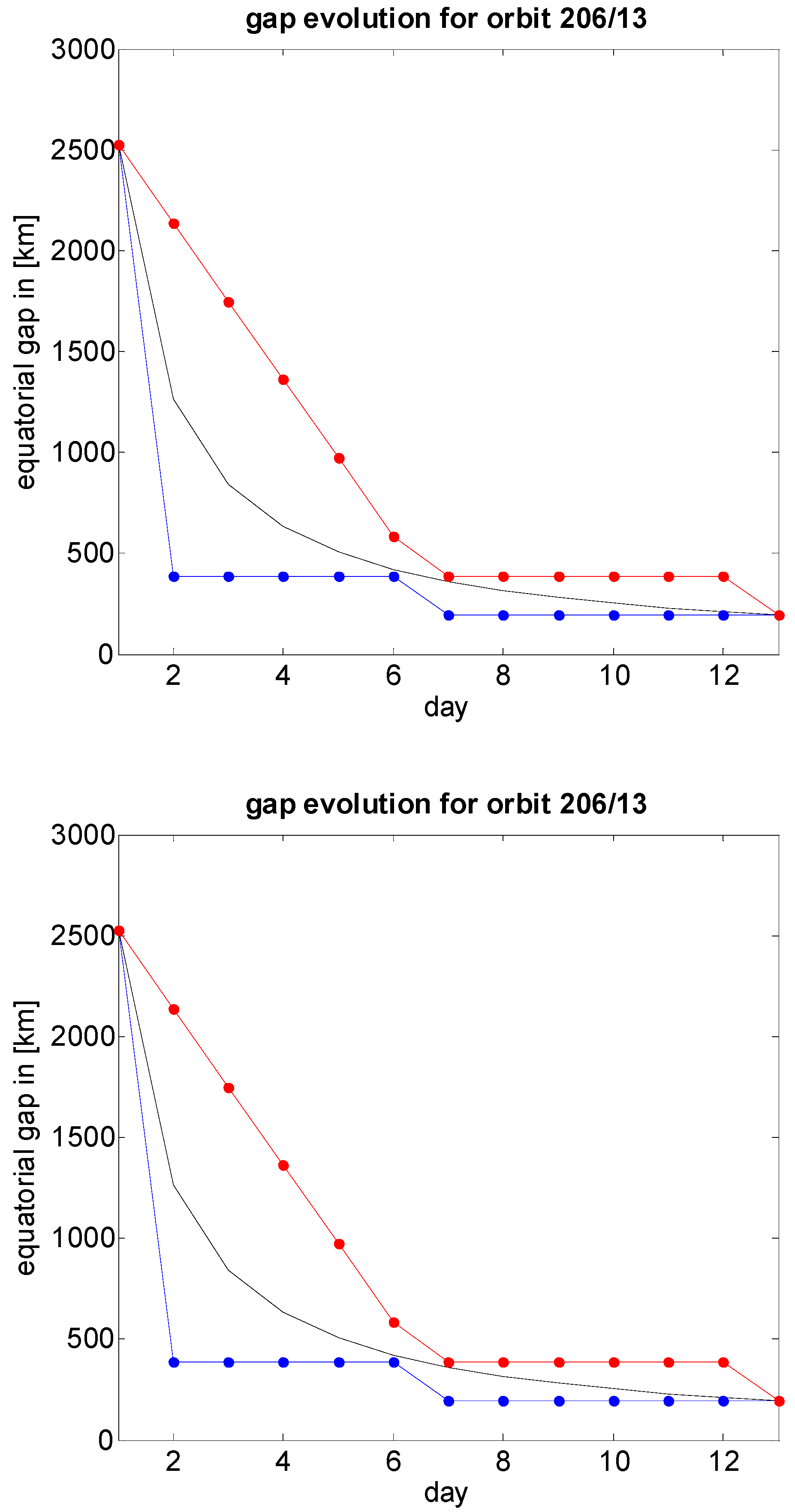
Here, we choose two mission scenarios from Table 2 for more detailed comparison and investigation. The scenarios have been selected such that they have almost the same altitudes; therefore, the mission height difference does not affect the performance. However, scenario a is in an odd parity orbit, whereas scenario b is in the even parity. Both orbits have almost similar groundtrack gap evolution and same sub-cycle of 6 days (Figure 7), but different full repeat cycles (13 days vs. 31 days). The performance of the mission choices are studied for two different formation flights (GRACE-like and Pendulum) and different angles of right ascension of the ascending node (RAAN). The choices of RAAN for the simulation start date of 1 January 1996 correspond to:
- -
- Ω = 0°: Starting from a point in Pacific Ocean, west of South-America,
- -
- Ω = 116°: Starting from a point in West-Africa,
- -
- Ω = 132°: Starting from a point in East-Africa.
GRACE-like (Inline) Formation
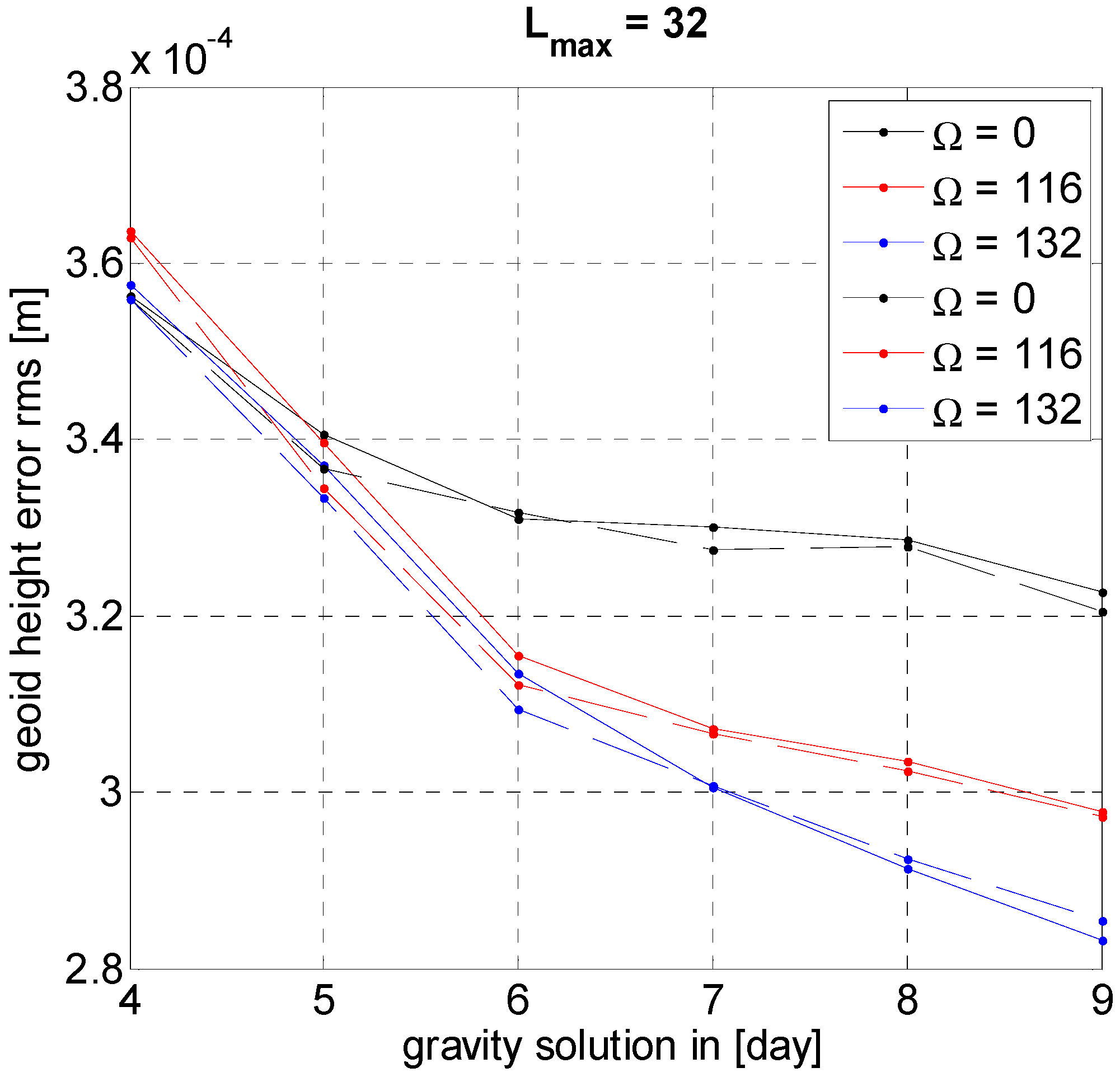
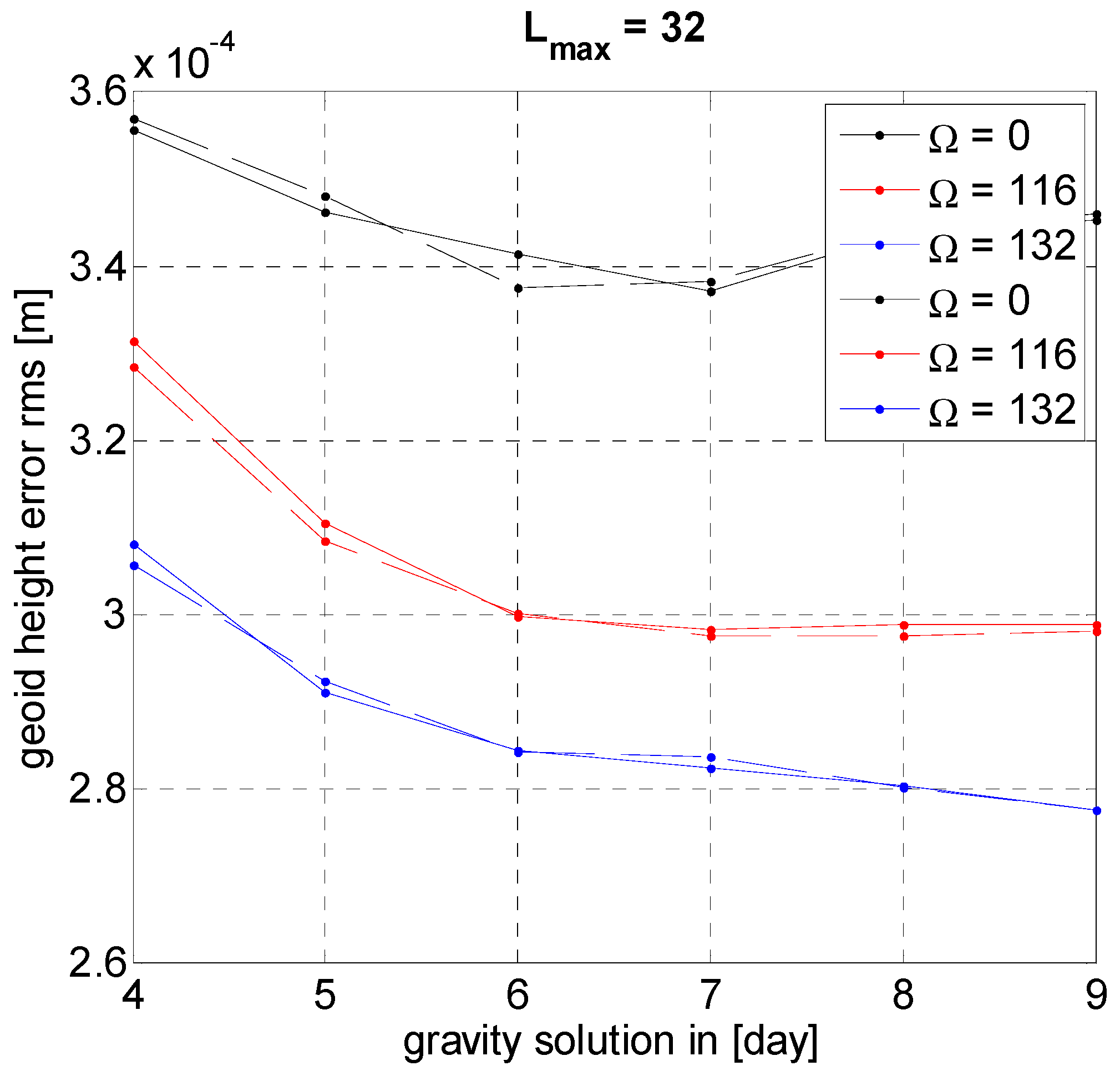
Figure 8 shows the gravity recovery of the GRACE-like scenarios a and b for Lmax = 32.
As we see in Figure 8, after the 5th day, the gravity recovery by Ω = 132° is better than Ω = 116°. The recovery by Ω = 0° is the worst. The odd parity scenario a usually performs a bit better than the even parity scenario b.
In terms of global recovery, the 6th day as sub-cycle period is not significant.
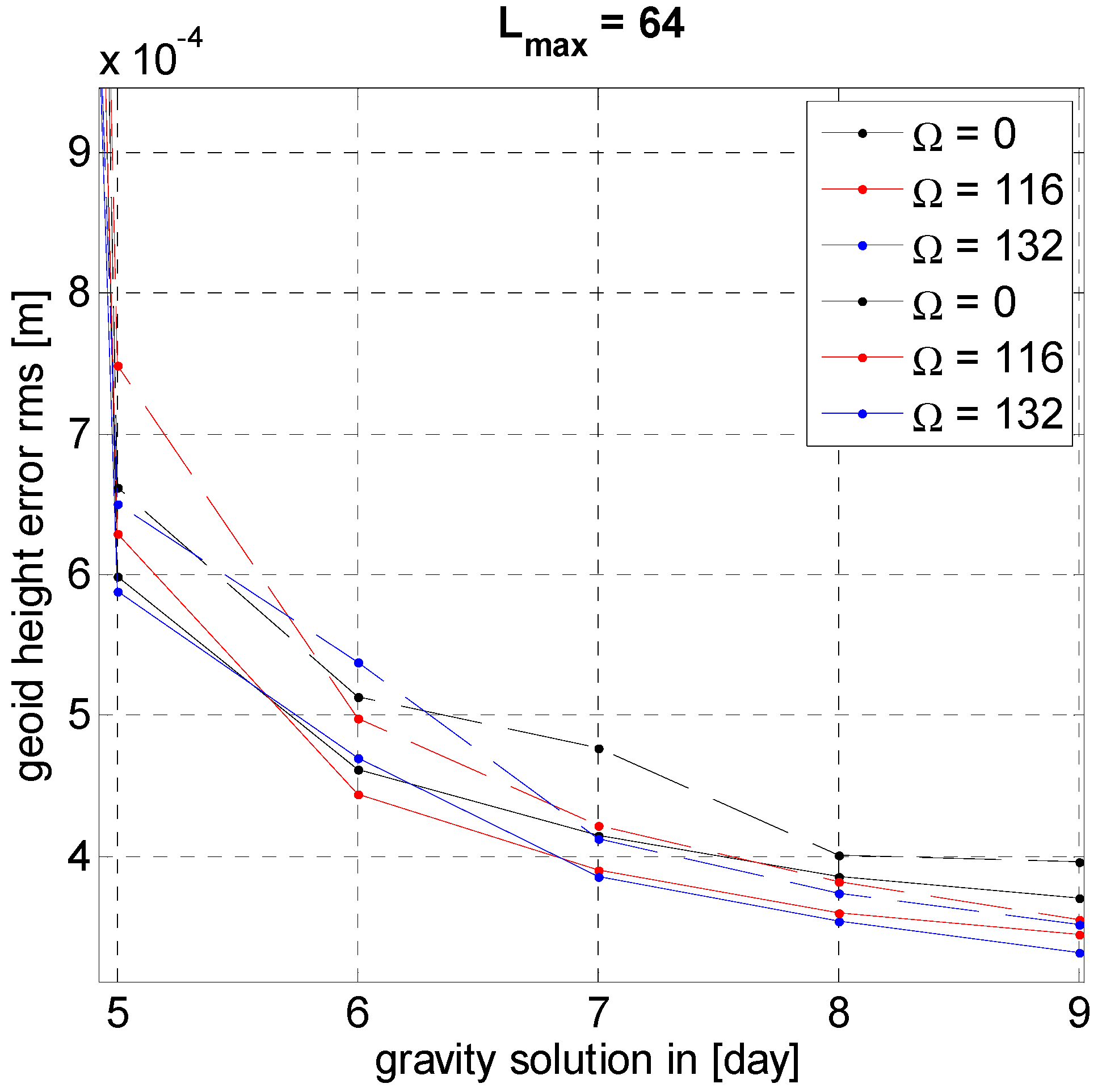
In case Lmax = 64, Figure 9 shows that the performance of the odd parity scenario is better than the even parity scenario, but the impact of Ω is not significant.
In terms of global recovery, the 6th day as sub-cycle period might be considered more significant for Lmax = 64 than the case of Lmax = 32.
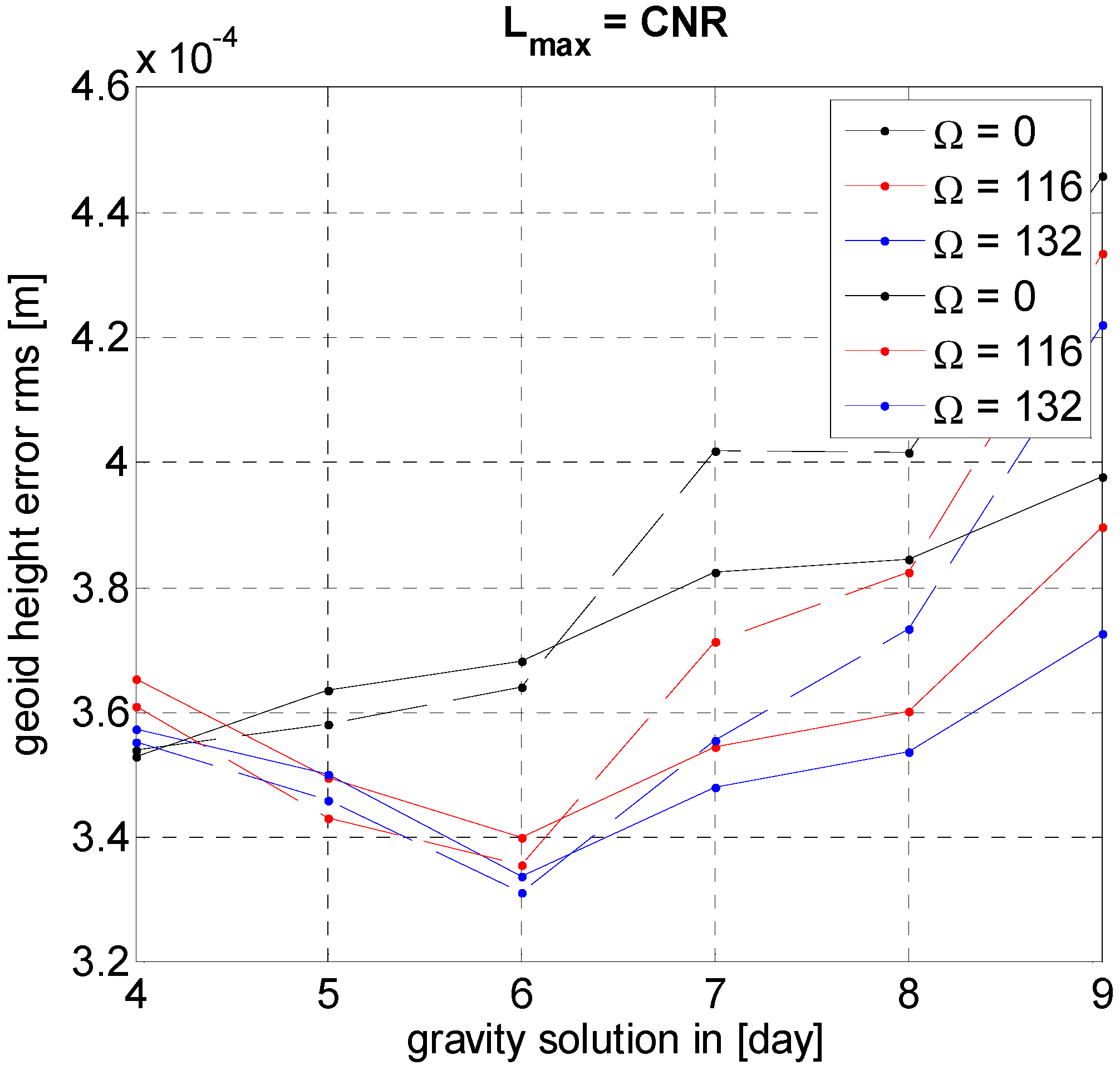
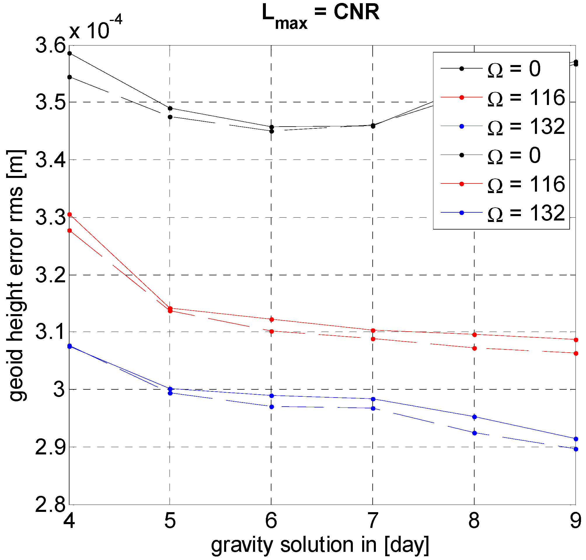
For Lmax = CNR, the dominant effect is the different impacts of odd and even parities on the gravity solutions larger than 7-day (Figure 10). Moreover, the impact of Ω can be seen (Ω = 132° usually performs better than Ω = 116°, and Ω = 0° is the worst).
In terms of global recovery, the 6th day as sub-cycle period has a significant influence. Afterwards, the error increases with the increase of time-interval of the solutions, which is very likely caused by the impact of temporal aliasing, since spatial aliasing is tried to be avoided (according to CNR).
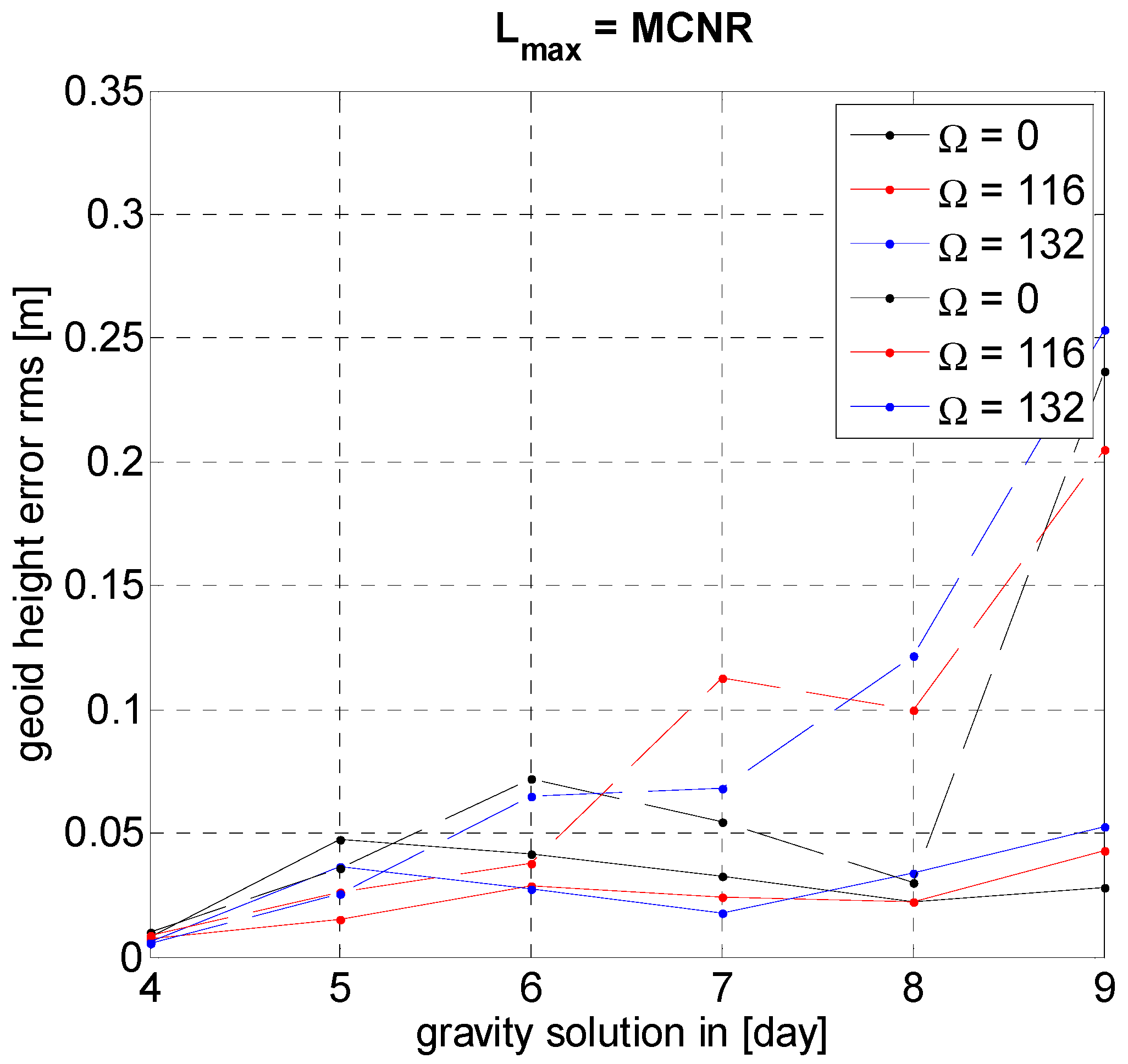
The case Lmax = MCNR is shown in Figure 11. The figure shows that above 6-day solutions, the odd parity scenario performs better than the even parity. Surprisingly, Ω = 0° performs almost the same as, or even better (for longer time solution) than, the others. Spatial aliasing is thought to be the biggest source of error, which increases as the time period of the gravity solutions increases (although temporal aliasing also exists, as for the other cases). Here, 6-day (as sub-cycle period) does not show important meaning. Possibly, the domination of spatial aliasing and the distribution of the geophysical signals with different strength over the globe hide the meaningful pattern.
Pendulum Formation
The addition of cross-track measurement of Pendulum formation to only along-track measurement of GRACE-like formation brings the expectation that Pendulum formation should reduce the recovery error through its more isotropic sampling behavior.
Figure 12, Figure 13, Figure 14 and Figure 15 illustrate the gravity recovery of scenarios a and b of Table 2 of a Pendulum formation, respectively for Lmax = 32, 64, CNR and MCNR. The average intersatellite distance of the two satellites in the formation is 100 km.
For Lmax = 32 in Figure 12, the recovery by Ω = 132° is better than Ω = 116°. The recovery by Ω = 0° is the worst and gets even worse at the longer periods. No significant difference is seen by the performance of the odd and even parities.
In terms of global recovery, the 6th day as sub-cycle period is not significantly important.
Figure 13 illustrates better performance in recovery quality by Ω = 132° than Ω = 116°. After 5-day, the gravity recovery by Ω = 0° is the worst, and gets even worse for the longer periods. No significant difference is seen by the performance of the odd and even parities, although the even parity performs only a bit better than the odd parity after 5-day. In terms of global recovery, the 6th day as sub-cycle period is not significantly important, although it shows a small impact on the recovery by Ω = 0° and Ω = 116°.
Unlike the case of CNR by the GRACE-like formation, the errors for Ω = 116° and Ω = 132° in Figure 14 decrease by the longer period of the solutions. One may associate this error reduction to the less spatial aliasing. However, that is not the case for Ω = 0°. The question is then how the combination of isotropy and sampling plays role.
Looking at the Figure 14, the Ω = 132° scenario shows better performance than Ω = 116° which outperforms Ω = 0°. Furthermore, the even parity performs a bit better than the odd parity.
In terms of global recovery, the 6th day as sub-cycle period is not significantly important.
In Figure 15 (MCNR case), the error increases for all cases after 6-day solution. In this case, extracting a meaning for sub-cycle (6-day) is not straightforward.
The odd parity outperforms the even parity at longer periods of solutions. The case Ω = 132° usually performs better than the two other cases.
3.1.2. Covariance Matrices
The illustration of the covariance matrices of the gravity solutions by different scenarios and cases can be employed as an indicator for the associated error levels, very much influenced by the geometry of the orbits and their sampling behaviors.
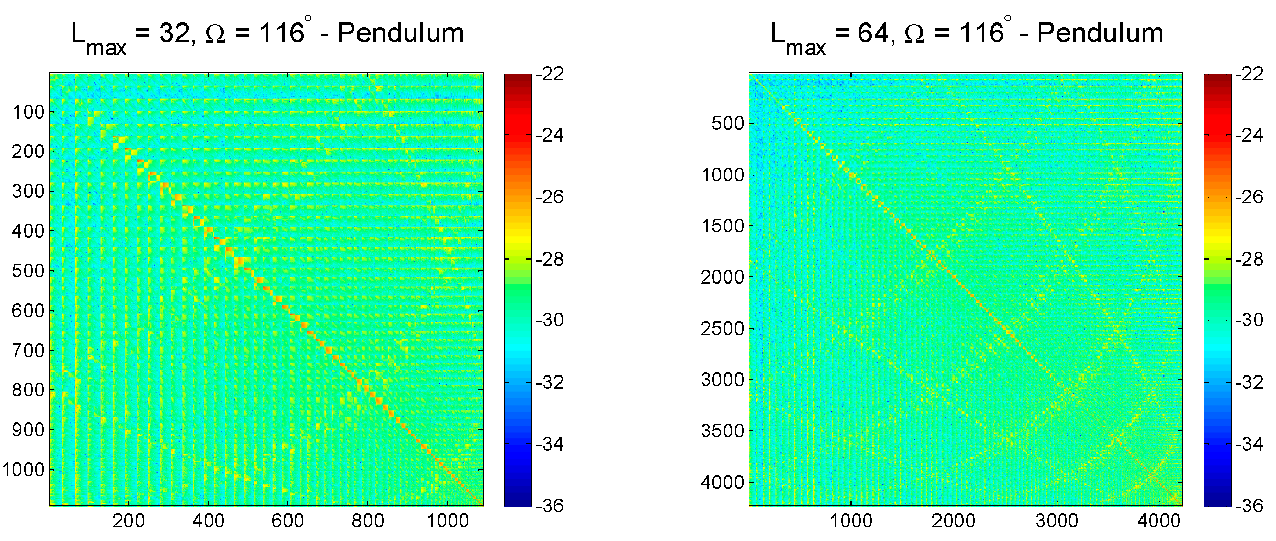
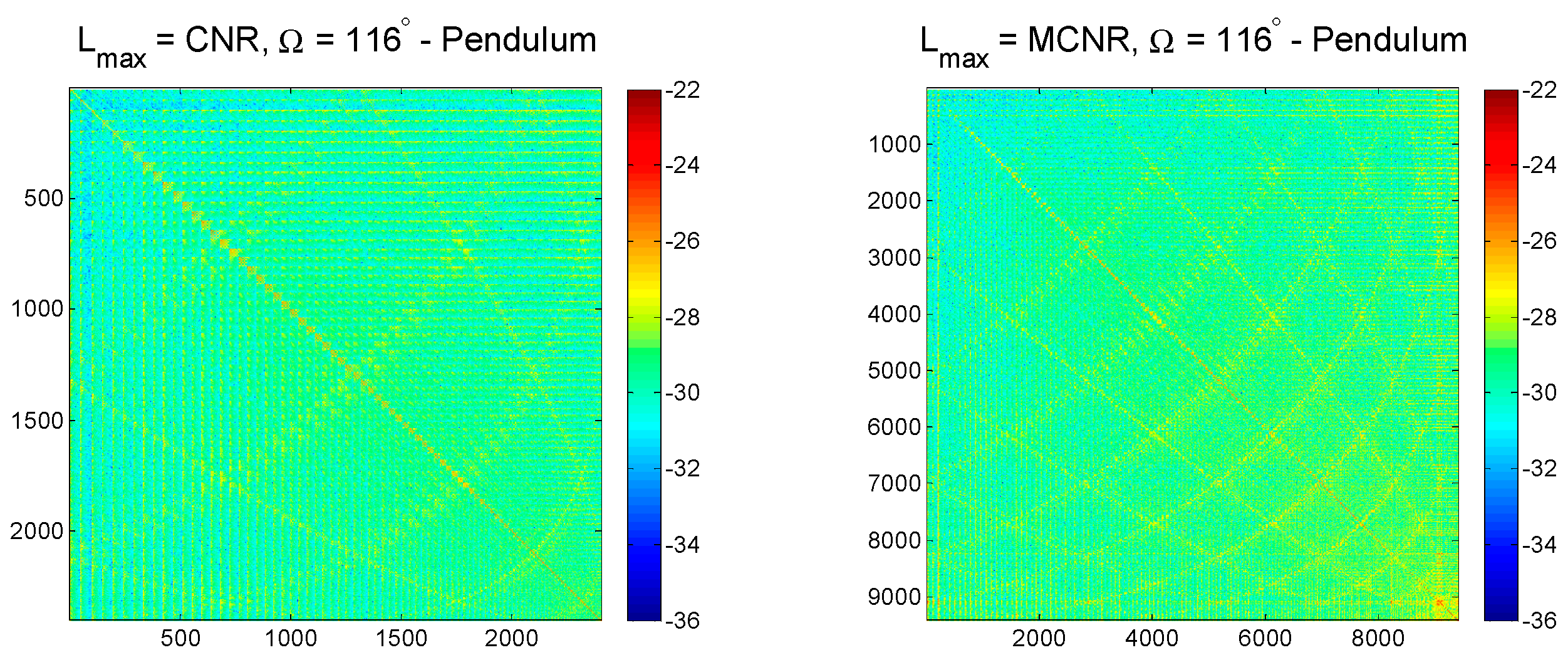
Figure 16 and Figure 17 depict the covariance matrices of 6-day solutions of the scenario (a) inline and Pendulum formations for Ω = 116°, up to Lmax = 32, Lmax = 64, Lmax = CNR and Lmax = MCNR solutions. The illustrations imply that for the inline formation when the maximum spherical harmonic degree and order goes above the CNR rule for 6-day (Lmax = 64 and Lmax = MCNR), the level of error shown by the arcs and off-diagonal elements (due to the spatial aliasing) gets significant. For the Pendulum formation, however, those error patterns are not as strong as the inline formation.
Inline (GRACE-like) Formation
Pendulum Formation
3.2. Mission Scenarios and the Regional Gravity Recovery
3.2.1. West Africa as an Example
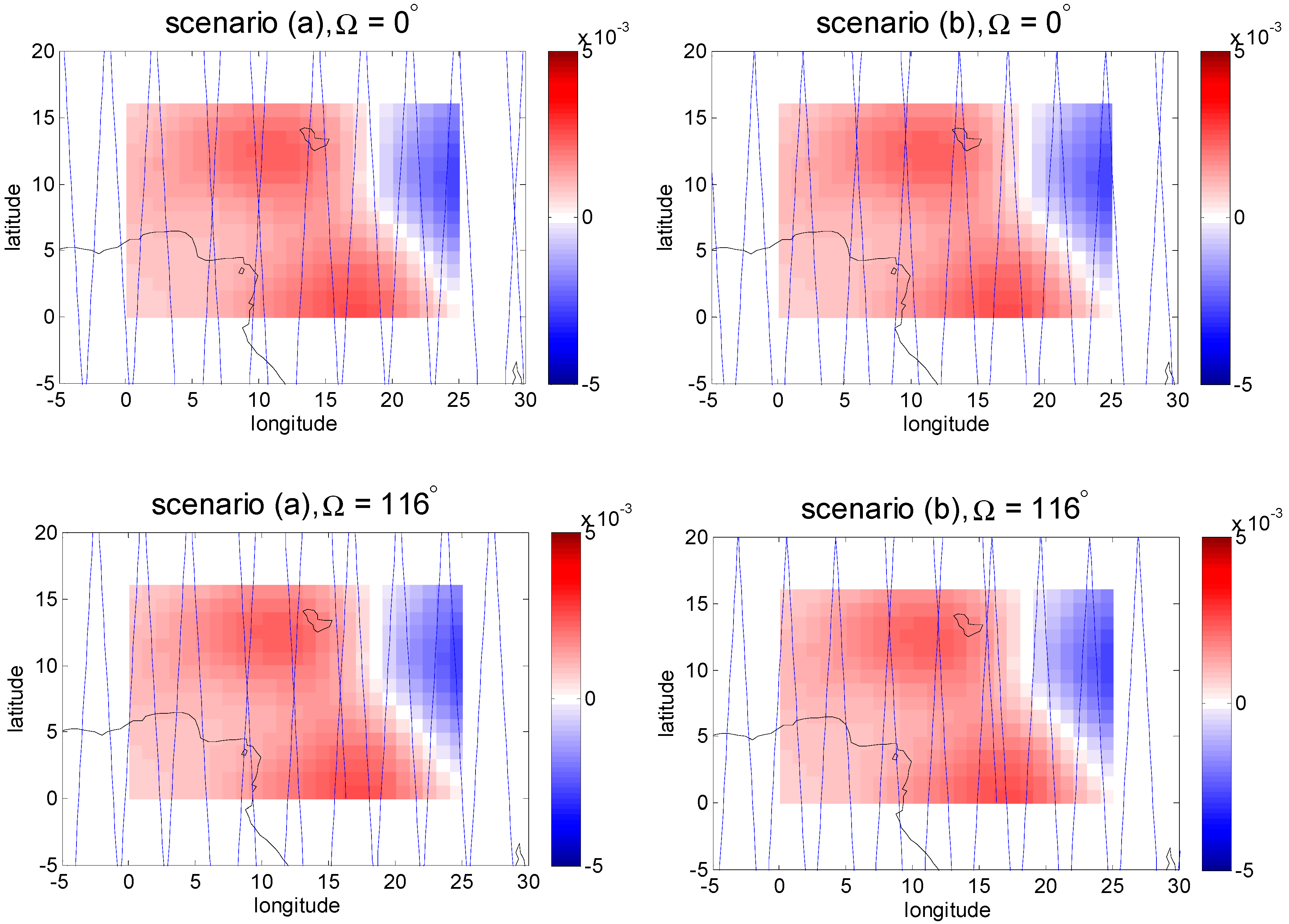
Two scenarios of Table 2 with almost same altitude and similar gap evolution (both has 6-day sub-cycle time-span) are investigated for their regional gravity recovery. Figure 18 depicts the groundtrack of the two scenarios on the selected area in West Africa for different RAAN angles after 6 days.
The error RMS of the gravity recovery in terms of geoid height for global and regional (West-Africa) 6-day solution of different cases are shown in Table 3, Table 4, Table 5, Table 6, Table 7, Table 8, Table 9 and Table 10. The results from the tables imply that the best global performance (the smallest error) usually happens at Ω = 132°. That might be expected, since among the three different Ω values, the mission track passes over the biggest signals when Ω = 132° (i.e., over East-Africa). In terms of regional investigation, the results are usually optimal when Ω = 116°. That is, in fact, the area where sub-cycle happens. However, for both global and regional cases, the above statements are not always valid. When the maximum spherical degree and order of the solution goes above the Colombo-Nyquist rule (CNR), exceptions can be observed. One possible explanation for those exceptions is the large spatial aliasing and the leakage from the surroundings which may deteriorates the impact of sub-cycle. Clearly, more detailed studies should be conducted in this direction.
The impact of the mission formation on the error can also be seen in the results. The outcomes show that the Pendulum formation usually outperforms the inline (GRACE-like) formation.
3.2.2. Spatial Covariance
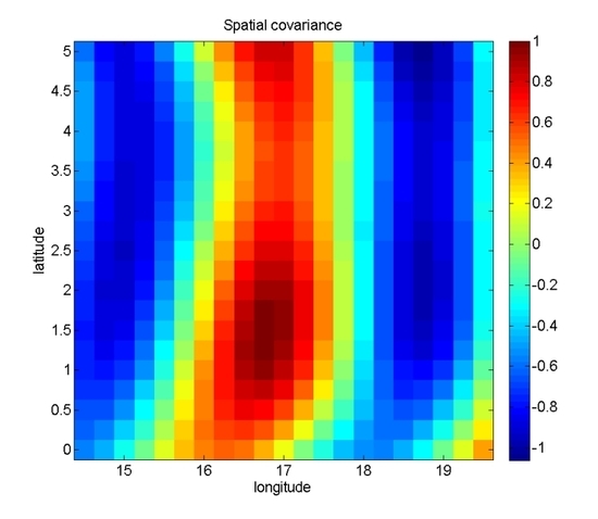
Another interesting tool to investigate the sampling impact is spatial covariance illustrations [29]. One may expect that denser sampling should result in more symmetric spatial covariance pattern.
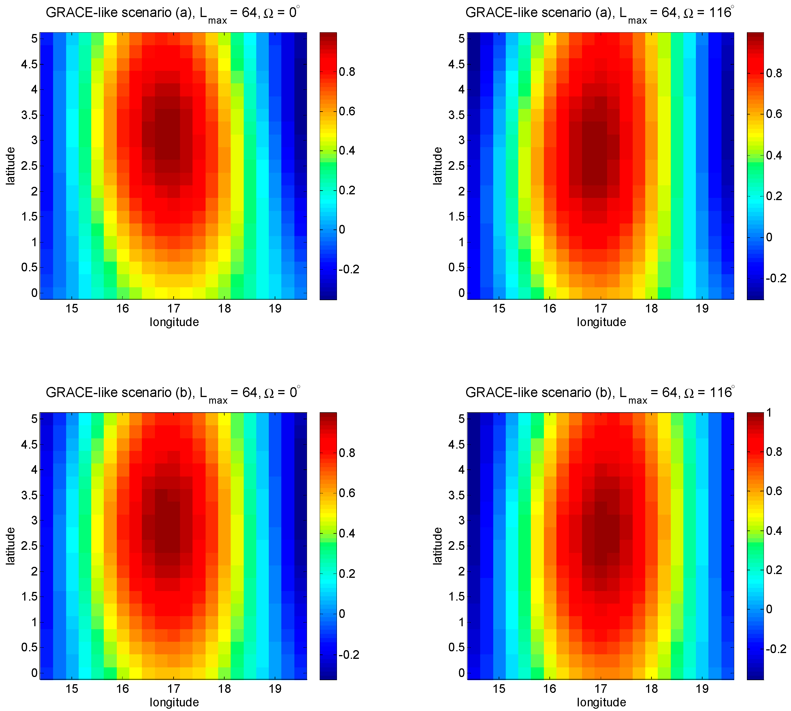
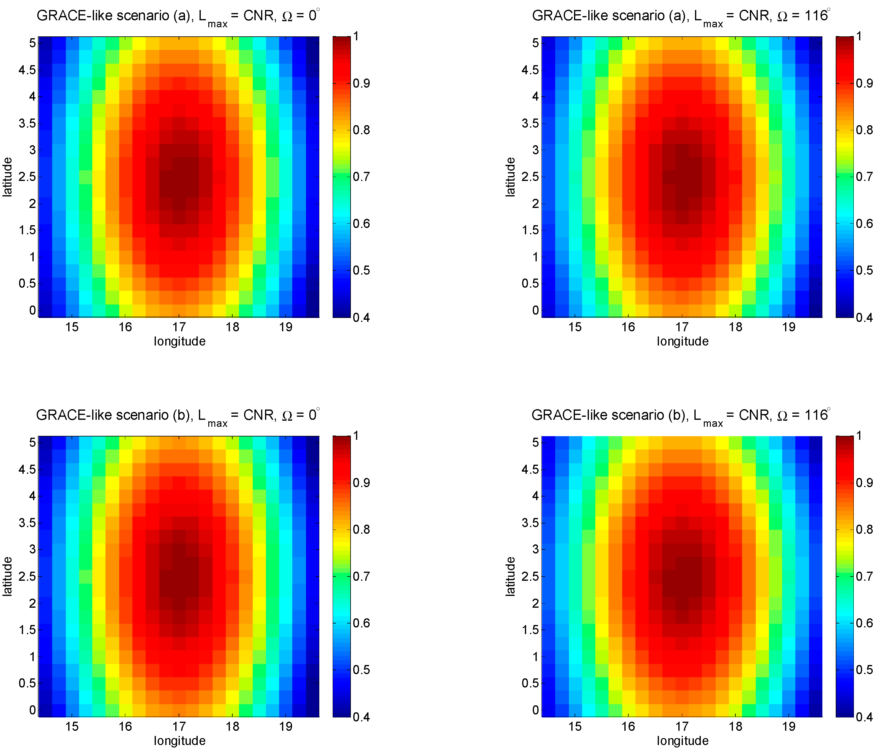
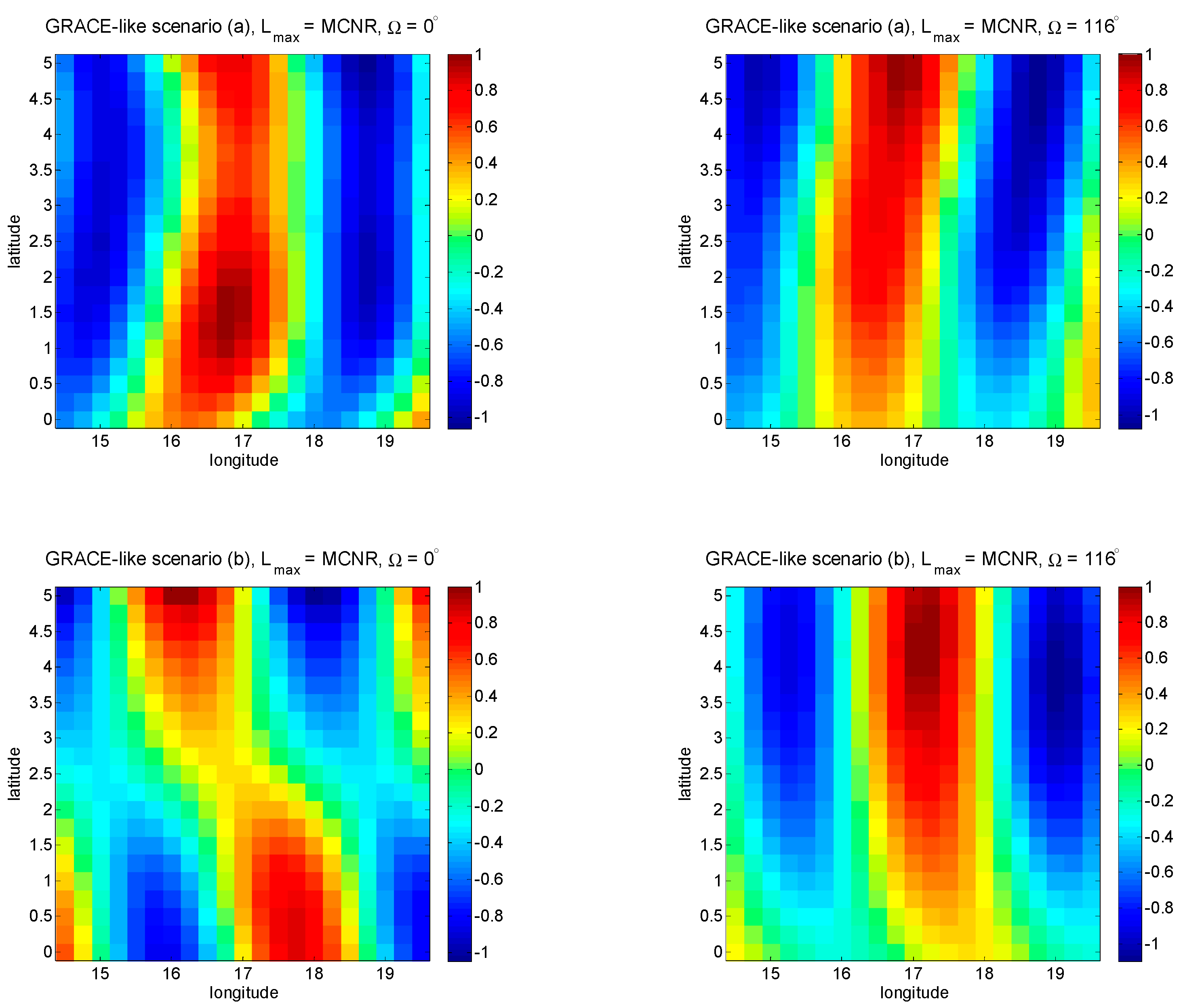
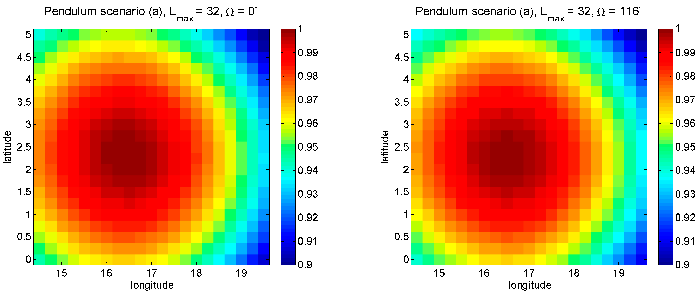
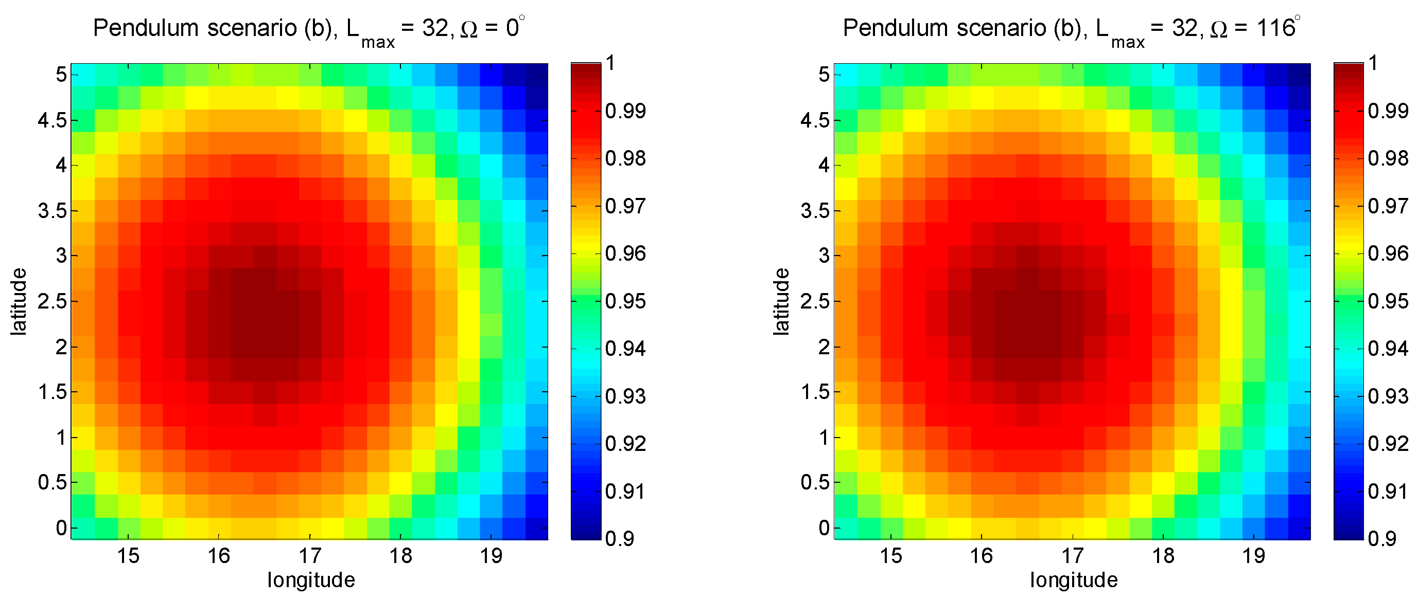
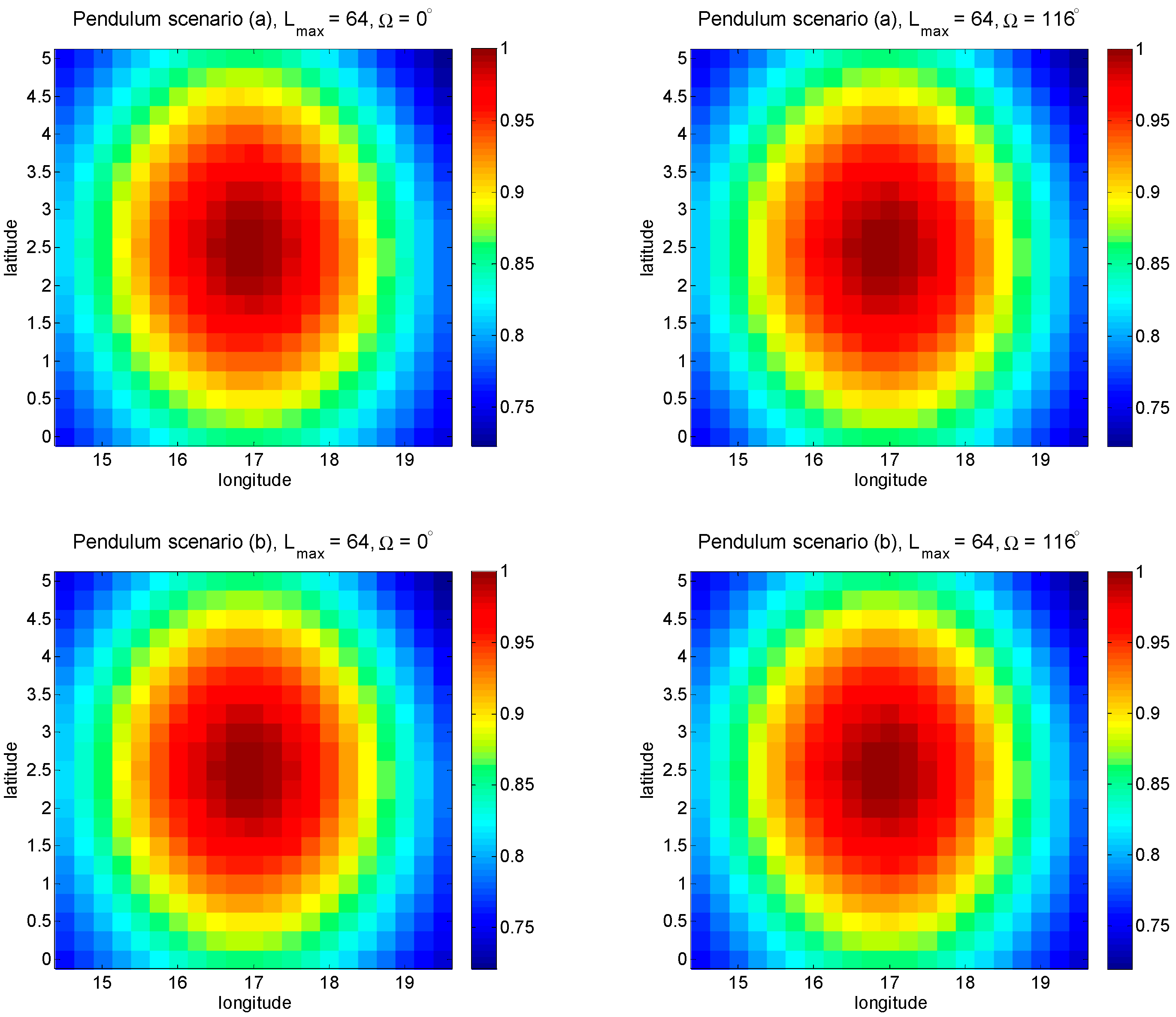
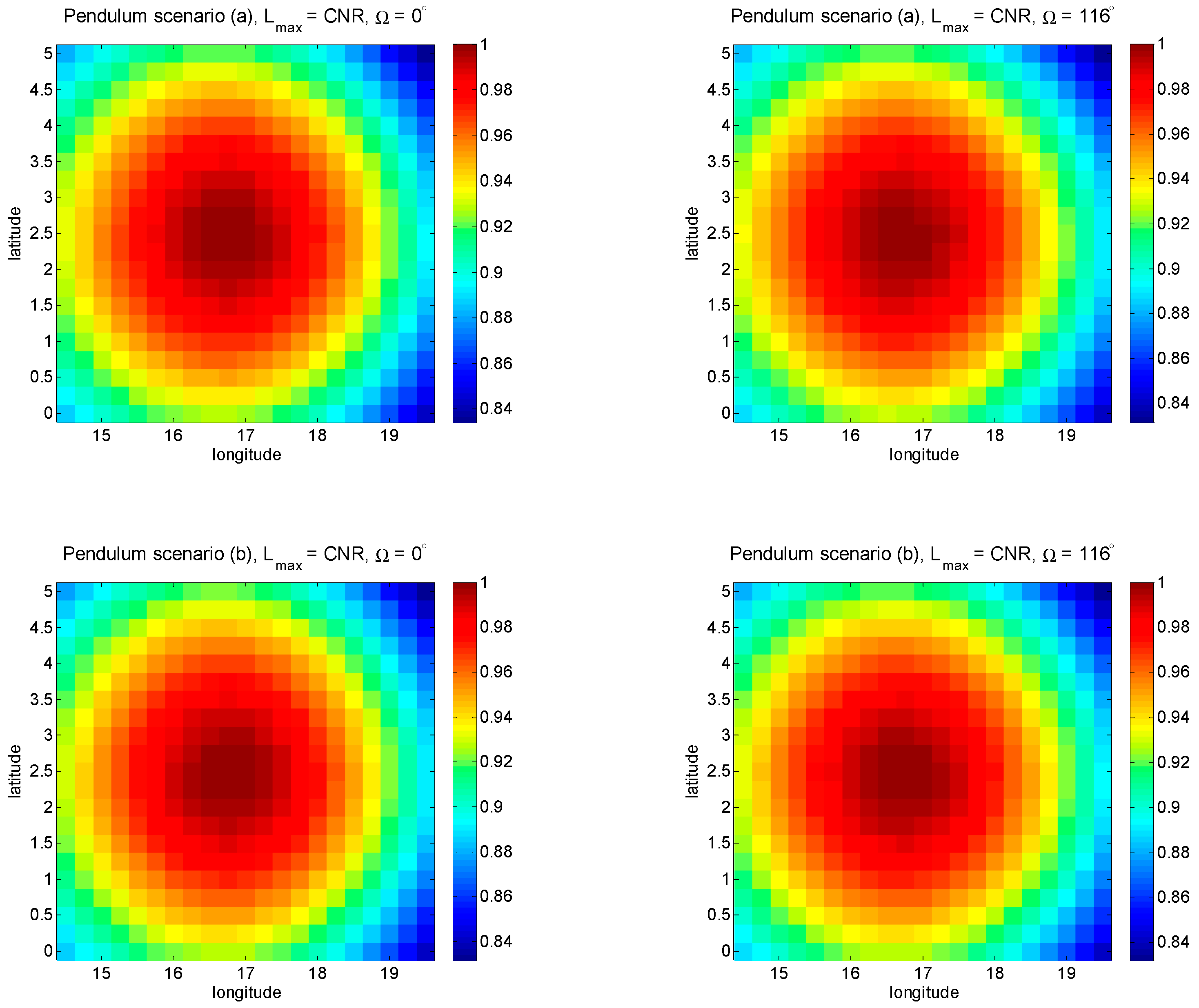
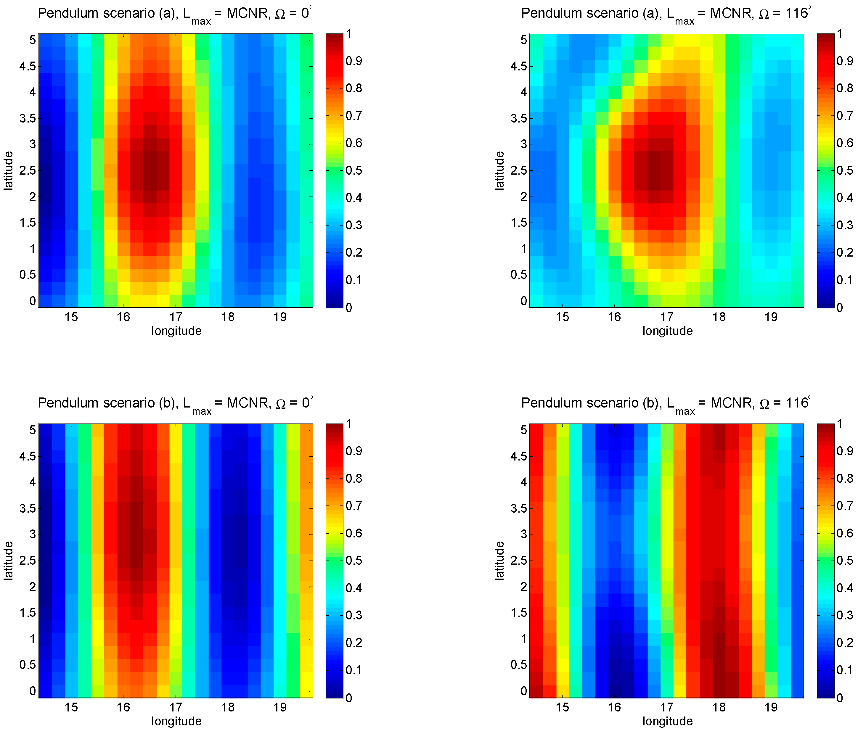
The spatial covariance patterns, centered on the selected points of Figure 19 and Figure 20 (marked by green star at longitude 17° and latitude 2.5°) for inline and Pendulum formations are depicted in Figure 21, Figure 22, Figure 23, Figure 24, Figure 25, Figure 26, Figure 27 and Figure 28 where two different RAAN angles (Ω = 0° and Ω = 116°) and different maximum spherical harmonic coefficient degrees and orders are addressed for 6-day solutions. The calculation of the spatial covariance is based on the work by [29].
The depicted results of the inline formation show the symmetry of the spatial covariance around the selected points for the cases Lmax = 32, 64 and CNR, although in the case of Lmax = 64 the spatial covariance graph center is shifted a bit from the center (in this case, the Ω = 116°, where sub-cycle happens, shows less affected than Ω = 0°). For the Pendulum formation, the graphs of Lmax = 32 and CNR show symmetric feature, but the graph centers are shifted towards left (more predominant for Lmax = 32). That is not the case for Lmax = 64. Interestingly, for the MCNR, the scenario a significantly outperforms the scenario b in terms of the symmetry.
Inline (GRACE-like) Formation
Pendulum Formation
4. Discussion
This work aimed to look more closely into the sampling patterns impact on the gravity recovery quality for global and regional studies, as the Colombo-Nyquist and modified Colombo-Nyquist rules apply. We tried to focus on the pure sampling impact in this paper, so no post-processing was considered. In reality, smoothing global or local filter (as one of the filter choices) is implemented. However, higher quality raw solutions (for example, due to denser sampling, and hence less spatial aliasing) can result in using more relaxed filters (e.g., a Gaussian smoothing with smaller radius). That would be then very beneficial in terms of signal-to-noise ratio, although the subject is outside the scope of this paper.
In particular, for the regional study, the groundtrack patterns impact of different satellite constellation scenarios have been investigated for a hydrological basin in central Africa. The quality of the gravity products have been assessed by different metrics such as spatial covariance representation. We also tried to investigate the potential meaning of the sub-cycle concept in terms of global and local impacts by different repeat-orbit scenarios with even and odd parities. Furthermore, different recovery scenarios in terms of the original and modified Colombo-Nyquist rules have been discussed.
The main points of our results can be summarized as follows:
In general, for 12 selected mission scenarios of Table 1:
For the case Lmax = 32, with the increase of the time-pan of the solutions, the recovery error decreases. This is because of more sampling in space, and hence, less spatial aliasing, although the temporal aliasing gradually increases (but not significantly). The same argument applies for the case Lmax = 64 as well. For Lmax = CNR and MCNR, it is generally different. That means that for most of the scenarios, the longer the recovery time-span, the bigger the error. But here, it is important to notice that different scenarios have different performances. For some scenarios of the case Lmax = CNR, the error increase is significant. The cause of such an increase should be associated with the spatial aliasing which is more predominant for some mission scenarios, most likely because of the geometry of their orbits and therefore their time evolution of their groundtracks. A similar statement also applies for the case MCNR, even though more fluctuations are seen in the recovery error of few scenarios.
In terms of global recovery and for the selected inline formation scenarios of Table 2:
Considering the inline formation missions, for Lmax = 32, the recovery by Ω = 132° after the 5th day is better than Ω = 116°. The recovery by Ω = 0° is the worst. Odd parity usually performs a bit better than the even parity. The 6th day as sub-cycle period is not significantly important in the global point of view. However, the concept might be more noticeable for Lmax = 64. For this case, the performance of the odd parity is better than the even parity. That is also the case for Lmax = CNR. In this case, different impact of odd and even parities on the gravity solutions larger than 7-day are significant. Moreover, the impact of Ω can be seen (Ω = 132° usually performs better than Ω = 116°, and Ω = 0° is the worst). In terms of global recovery, the 6th day as sub-cycle period also has a significant influence. After the 6th day, the error increases with the increase of the recovery time-interval. This effect is mainly assumed to be associated with the impact of temporal aliasing, since the spatial aliasing is tried to be largely avoided, according to CNR (although the spatial aliasing still exits by the impact of orbit geometry).
For the MCNR recovery, the odd parity performs better than the even parity above 6-day solutions. Surprisingly, Ω = 0° performs almost equal or even better (for longer time recovery) than the other two cases. Spatial aliasing is thought to be the biggest source of the error which increases as time span of the solutions increases (although temporal aliasing also contributes, as it is valid for all the other cases).
6-day (as sub-cycle period) does not show noticeable meaning. Very likely, the domination of spatial aliasing and the distribution of the geophysical signals with different strength over the globe hinder the emergence of any meaningful pattern.
Considering the Pendulum formation of the Table 2 scenarios, and in the terms of global recovery, for the Lmax = 32, Ω = 132° performs better than Ω = 116°. The recovery by Ω = 0° is the worst and getting even worse over longer periods. One can not see significant difference by the performance of the odd and even parities. The 6th day as sub-cycle period is not significantly important in this case. For Lmax = 64, the recovery by Ω = 132° is better than Ω = 116°. After day 5, recovery by Ω = 0° is the worst and getting even worse at the longer periods. No significant difference is seen by the performance of the odd and even parities, although the even parity performs only a bit better than the odd parity after day 5. In terms of global recovery, the 6th day as sub-cycle period shows no important feature, although it may depict a very small impact on the recovery by Ω = 0° and Ω = 116°.
Unlike the case of CNR by inline formation, reduction of errors for Ω =116° and Ω = 132° by the longer period of the solutions are seen (possibly by less spatial aliasing). However, that is not the case for Ω = 0°. Therefore, one potential question to be addressed in future works might be the way that combination of isotropy (by Pendulum formation) and sampling plays role. The Ω = 132° case performs better than Ω = 116° which outperforms Ω = 0°. The even parity illustrates a slightly better performance than the odd parity. In terms of global recovery, the 6th day (as sub-cycle period) should not be considered significantly important.
For the MCNR case, the error increases for all cases after the 6-day solution. Therefore, it is not clear whether day 6 has meaning in terms of being sub-cycle or not. It is noticeable to see the better performance of the odd parity than the even parity at longer periods of solutions. The case Ω = 132° mostly performs better than the two other cases.
This paper also illustrates covariance matrices for 6-day solutions of the scenario (a) inline and Pendulum formations for Ω = 116°, where Lmax = 32, Lmax = 64, Lmax = CNR and Lmax = MCNR. The illustrations show that for the inline formation when the maximum spherical harmonic coefficient degree and order are above the CNR rule for 6-day (i.e., Lmax = 64 and Lmax = MCNR), the error level gets significant (assumed to be associated with spatial aliasing). However, for the Pendulum formation, those error patterns are not as noticeable as the inline formation (very likely associated to the more isotropic sampling by Pendulum formation).
Interpreting the results above, it should be emphasized that with our starting date choice for recovery simulation (1 January 1996), Ω = 0° corresponds to the groundtrack starting point at Pacific Ocean, east of South America, while Ω = 116° and Ω = 132° respectively stand for starting points at West-Africa and East-Africa. The results of this paper show that the best global performance (the smallest error) usually happens at Ω = 132°. This outcome might be expected since, among the three different values of Ω, the satellite mission track passes over significant hydrological signals when Ω = 132° (i.e., over East-Africa and the corresponding regions in the same longitudes). In terms of regional investigation, the results are usually optimal for the Ω = 116° case. In fact, this outcome is also expected, since that is the area where sub-cycle happens for the region targeted in this study (West-Africa). Nevertheless, for both global and regional study, the above statements are not always valid. When the maximum spherical degree and order of the solution goes beyond the Colombo-Nyquist rule (CNR), exceptions can be observed. A possible explanation for those exceptions could be the large spatial aliasing and the leakage from the surroundings which very likely deteriorates the impact of the sub-cycle. Obviously, more detailed studies should be directed in this way.
The results of our study also emphasize the impact of the mission formation on the error, where the Pendulum formation usually outperforms the inline (GRACE-like) formation, as expected through its more isotropic sampling behavior.
The spatial covariance illustrations of this research work for the GRACE-like formation depict the symmetry of the spatial covariance around the selected points for the cases Lmax = 32, 64, and CNR, although in the case of Lmax = 64, the spatial covariance graph center is shifted a bit, although for the Ω = 116° (where sub-cycle happens) the shift is less noticeable than for Ω = 0°. For the Pendulum formation, the graphs of Lmax = 32 and CNR feature symmetric patterns, but the graph centers are shifted towards left where it is more predominant for Lmax = 32. That is not the case for maximum spherical harmonic coefficient 64. It is interesting to say that for the MCNR recovery, the scenario (a) significantly outperforms the scenario (b) in terms of the symmetry.
Regarding the orbit parity impact on the gravity recovery, one should notice that the parity state (odd or even) is usually meaningful for the full repeat cycle. However, the evolution of the groundtrack pattern before the full cycle might be sophisticated and differ in each case; hence it is more reasonable to see the impact by its association to the groundtrack pattern distribution at a specific time span. That means, for the recovery time-spans shorter than the full-repeat cycle, instead of talking about the parity impact on the gravity recovery, it makes more sense to study the groundtrack pattern at that specific time interval and look for its potential association with the recovery quality. This issue will be addressed in our future works in more detail.
5. Conclusions
This paper examines the impact of sampling patterns on gravity recovery quality for global and regional studies when the Colombo-Nyquist and modified Colombo-Nyquist rules apply. For the regional study, the groundtrack pattern impact of different satellite constellation scenarios have been studied for a hydrological basin in central Africa. The quality of the gravity products were assessed by different metrics, e.g., by spatial covariance representation. The possible meaning of the sub-cycle concept in terms of global and local impacts was also investigated by different repeat-orbit scenarios with even and odd parities where different solution scenarios in terms of the original and modified Colombo-Nyquist rules have been discussed. Our results emphasize the impact of maximum harmonics of the recovery (both global and regional), the influence of sub-cycle on local gravity recovery, and the mission formation impact on recovery error.
Author Contributions
Conceptualization, S.I.-P.; Methodology, S.I.-P., M.W. and N.S.; Software, S.I.-P., M.W. and N.S.; Analysis, S.I.-P.; Writing-Original Draft Preparation, S.I.-P.; Writing-Review and Editing, S.I.-P., M.W. and A.A-S.; Visualization, S.I.-P.
Funding
This research was funded by Iranian National Elites Foundation as a grant for guest researchers at University of Isfahan, Iran.
Conflicts of Interest
The authors declare no conflicts of interest.
References
- Sharifi, M.; Sneeuw, N.; Keller, W. Gravity recovery capability of four generic satellite formations. In Proceedings of the 1st International Symposium of the International Gravity Field Service “Gravity Field of the Earth”, Porto, Portugal, 28 August–1 September 2006; pp. 211–216. [Google Scholar]
- Bender, P.; Wiese, D.; Nerem, R. A possible dual-GRACE mission with 90 degree and 63 degree inclination orbits. In Proceedings of the Third International Symposium on Formation Flying, Missions and Technologies, Noordwijk, The Netherlands, 23–25 April 2008; European Space Agency: Noordwijk, The Netherlands, 2008; pp. 1–6. [Google Scholar]
- Wiese, D.; Folkner, W.; Nerem, R. Alternative mission architectures for a gravity recovery satellite mission. J. Geodesy 2009, 83, 569–581. [Google Scholar] [CrossRef]
- Elsaka, B. Simulated Satellite Formation Flights for Detecting Temporal Variations of the Earth’s Gravity Field. Ph.D. Thesis, University of Bonn, Bonn, Germany, 2010. [Google Scholar]
- Wiese, D.; Nerem, R.; Lemoine, F. Design considerations for a dedicated gravity recovery satellite mission consisting of two pairs of satellites. J. Geodesy 2012, 86, 81–98. [Google Scholar] [CrossRef]
- Ellmer, M. Optimization of the Orbit Parameters of Future Gravity Missions Using Genetic Algorithms. Master’s Thesis, University of Stuttgart, Stuttgart, Germany, 2011. [Google Scholar]
- Elsaka, B.; Kusche, J.; Ilk, K. Recovery of the Earth’s gravity field from formation-flying satellites: Temporal aliasing issues. Adv. Space Res. 2012, 50, 1534–1552. [Google Scholar] [CrossRef]
- Iran Pour, S.; Reubelt, T.; Sneeuw, N. Quality assessment of sub-Nyquist recovery from future gravity satellite missions. Adv. Space Res. 2013, 52, 916–929. [Google Scholar] [CrossRef]
- Reubelt, T.; Sneeuw, N.; Iran Pour, S.; Hirth, M.; Fichter, W.; Müller, J.; Brieden, P.; Flechtner, F.; Raimondo, J.-C.; Kusche, J.; et al. Future gravity field satellite missions. In Observation of the System Earth from Space-CHAMP, GRACE, GOCE and Future Missions; Springer: Berlin, Germany, 2013; pp. 165–230. [Google Scholar]
- Elsaka, B.; Raimondo, J.-C.; Brieden, P.; Reubelt, T.; Kusche, J.; Flechtner, F.; Iran Pour, S.; Sneeuw, N.; Müller, J. Comparing seven candidate mission configurations for temporal gravity field retrieval through full-scale numerical simulation. J. Geodesy 2014, 88, 31–43. [Google Scholar] [CrossRef]
- Baldesarra, M.; Brieden, P.; Danzmann, K.; Daras, I.; Doll, B.; Feili, D.; Flechtner, F.; Flury, J.; Gruber, T.; Sneeuw, N.; et al. e2motion—Earth System Mass Transport Mission—Concept for a Next Generation Gravity Field Mission; Deutsche Geodätische Kommission der Bayerischen Akademie der Wissenschaften, Reihe B, Angewandte Geodäsie 318; Deutsche Geodätische Kommission der Bayerischen Akademie der Wissenschaften: Munich, Germany, 2014. [Google Scholar]
- Klokočník, J.; Wagner, C.; Kostelecký, J.; Bezděk, A. Ground track density considerations on the resolvability of gravity field harmonics in a repeat orbit. Adv. Space Res. 2015, 56, 1146–1160. [Google Scholar] [CrossRef]
- Iran Pour, S.; Weigelt, M.; Reubelt, T.; Sneeuw, N. Impact of groundtrack pattern of double pair missions on the gavity recovery quality: Lessons from the ESA SC4MGV project. Int. Symp. Earth Environ. Sci. Future Gener. 2016, 147, 97–101. [Google Scholar]
- Anselmi, A.; Visser, P.; van Dam, T.; Sneeuw, N.; Gruber, T.; Altès, B.; Christophe, B.; Cossu, F.; Ditmar, P.G.; Murbock, M.; et al. Assessment of a Next Generation Gravity Mission to Monitor the Variations of Earth’s Gravity Field; European Space Agency (ESA), ESA-ESTEC: Noordwijk, The Netherlands, 2011. [Google Scholar]
- Iran Pour, S.; Reubelt, T.; Sneeuw, N.; Daras, L.; Murböck, M.; Gruber, T.; Pail, R.; Weight, M.; Van Dam, T.; VIsser, P.; et al. ESA SC4MGV Project “Assessment of Satellite Constellations for Monitoring the Variations in Earth’s Gravity Field"; European Space Agency (ESA), ESA-ESTEC: Noordwijk, The Netherlands, 2015. [Google Scholar]
- Van Dam, T.; Visser, P.; Sneeuw, N.; Losch, M.; Gruber, T.; Bamber, J.; Bierkens, M.; Smit, M. Monitoring and Modelling Individual Sources of Mass Distribution and Transport in the Earth System by Means of Satellites; European Space Agency (ESA), ESA-ESTEC: Noordwijk, The Netherlands, 2008. [Google Scholar]
- Reubelt, T.; Sneeuw, N.; Iran-Pour, S. Quick-look gravity field analysis of formation scenarios selection. Geotechnol. Sci. Rep. 2010, 17, 126–133. [Google Scholar]
- Colombo, O. The Global Mapping of Gravity with Two Satellites, 3rd ed.; Netherlands Geodetic Commission: Amersfoort, The Netherlands, 1984. [Google Scholar]
- Sneeuw, N. A Semi-Analytical Approach to Gravity Field Analysis from Satellite Observations; Universitätsbibliothek der TU München: Munich, Germany, 2000. [Google Scholar]
- Visser, P.; Schrama, E.; Sneeuw, N.; Weigelt, M. Dependency of resolvable gravitational spatial resolution on Space-Borne observation techniques. In Geodesy for Planet Earth; Springer: Berlin, Germany, 2012; pp. 373–379. [Google Scholar]
- Weigelt, M.; Sneeuw, N.; Schrama, E.; Visser, P. An improved sampling rule for mapping geopotential functions of a planet from a near polar orbit. J. Geodesy 2012, 87, 127–142. [Google Scholar] [CrossRef] [Green Version]
- Wiese, D.; Visser, P.; Nerem, R. Estimating low resolution gravity fields at short time intervals to reduce temporal aliasing errors. Adv. Space Res. 2011, 48, 1094–1107. [Google Scholar] [CrossRef]
- Dobslaw, H.; Bergmann-Wolf, I.; Dill, R.; Forootan, E.; Klemann, V.; Kusche, J.; Sasgen, I. The updated ESA Earth System Model for future gravity mission simulation studies. J. Geodesy 2015, 89, 505–513. [Google Scholar] [CrossRef]
- Gruber, T.; Bamber, J.L.; Bierkens, M.F.P.; Dobslaw, H.; Murböck, M.; Thomas, M.; Van Beek, L.P.H.; Van Dam, T.; Visser, P. Simulation of the time-variable gravity field by means of coupled geophysical models. Earth Syst. Sci. Data 2011, 3, 19–35. [Google Scholar] [CrossRef] [Green Version]
- Savcenko, R.; Bosch, W. EOT08a-Empirical Ocean Tide Model from Multi-Mission Satellite Altimetry; Deutsches Geodätisches Forschungsinstitut (DGFI): München, Germany, 2008. [Google Scholar]
- Ray, R.; NASA Goddard Space Flight Center, Washington, Maryland, USA. Private communication, 2008.
- Visser, P.; Sneeuw, N.; Reubelt, T.; Losch, M.; van Dam, T. Space-borne gravimetric satellite constellations and ocean tides: Aliasing effects. Geophys. J. Int. 2010, 181, 789–805. [Google Scholar] [CrossRef] [Green Version]
- Hill, G. Researches in the lunar theory. Am. J. Math. 1878, 1, 5–26. [Google Scholar] [CrossRef]
- Haagmans, R.; van Gelderen, M. Error variances-covariances of GEM-T1: Their characteristics and implications in geoid computation. Geophys. Res. Solid Earth 1991, 96, 20011–20022. [Google Scholar] [CrossRef]
Figure 1.
Error RMS in terms of geoid height for the gravity solutions of the Table 1 mission scenarios for maximum spherical harmonic degree and order 32.
Figure 1.
Error RMS in terms of geoid height for the gravity solutions of the Table 1 mission scenarios for maximum spherical harmonic degree and order 32.

Figure 2.
Error RMS in terms of geoid height for the gravity solutions of the Table 1 mission scenarios for maximum spherical harmonic degree and order 64.
Figure 2.
Error RMS in terms of geoid height for the gravity solutions of the Table 1 mission scenarios for maximum spherical harmonic degree and order 64.

Figure 3.
The zoom-in graph of the Figure 2.
Figure 3.
The zoom-in graph of the Figure 2.

Figure 4.
Error RMS in terms of geoid height for the gravity solutions of the Table 1 mission scenarios for maximum spherical harmonic degree and order CNR.
Figure 4.
Error RMS in terms of geoid height for the gravity solutions of the Table 1 mission scenarios for maximum spherical harmonic degree and order CNR.

Figure 5.
Error RMS in terms of geoid height for the gravity solutions of the Table 1 mission scenarios for maximum spherical harmonic degree and order MCNR.
Figure 5.
Error RMS in terms of geoid height for the gravity solutions of the Table 1 mission scenarios for maximum spherical harmonic degree and order MCNR.

Figure 6.
The zoom-in graph of the Figure 5.
Figure 6.
The zoom-in graph of the Figure 5.

Figure 7.
Gap evolution graphs for the repeat orbits of the Table 2 mission scenarios. The blue, red and black curves show the minimum, maximum and average unobserved gaps for each day, respectively.
Figure 7.
Gap evolution graphs for the repeat orbits of the Table 2 mission scenarios. The blue, red and black curves show the minimum, maximum and average unobserved gaps for each day, respectively.

Figure 8.
Global error RMS in terms of geoid height for odd (solid line) and even (dashed line) parities (inline scenarios a and b of the Table 2, respectively) for the gravity solutions up to maximum spherical harmonic degree and order 32. Different colors stand for different Ω.
Figure 8.
Global error RMS in terms of geoid height for odd (solid line) and even (dashed line) parities (inline scenarios a and b of the Table 2, respectively) for the gravity solutions up to maximum spherical harmonic degree and order 32. Different colors stand for different Ω.

Figure 9.
Global error RMS in terms of geoid height for odd (solid line) and even (dashed line) parities (inline scenarios a and b of the Table 2, respectively) for the gravity solutions up to maximum spherical harmonic degree and order 64. Different colors stand for different Ω.
Figure 9.
Global error RMS in terms of geoid height for odd (solid line) and even (dashed line) parities (inline scenarios a and b of the Table 2, respectively) for the gravity solutions up to maximum spherical harmonic degree and order 64. Different colors stand for different Ω.

Figure 10.
Global error RMS in terms of geoid height for odd (solid line) and even (dashed line) parities (inline scenarios a and b of the Table 2, respectively) for the gravity solutions up to maximum spherical harmonic degree and order CNR. Different colors stand for different Ω.
Figure 10.
Global error RMS in terms of geoid height for odd (solid line) and even (dashed line) parities (inline scenarios a and b of the Table 2, respectively) for the gravity solutions up to maximum spherical harmonic degree and order CNR. Different colors stand for different Ω.

Figure 11.
Global error RMS in terms of geoid height for odd (solid line) and even (dashed line) parities (inline scenarios a and b of the Table 2, respectively) for the gravity solutions up to maximum spherical harmonic degree and order MCNR. Different colors stand for different Ω.
Figure 11.
Global error RMS in terms of geoid height for odd (solid line) and even (dashed line) parities (inline scenarios a and b of the Table 2, respectively) for the gravity solutions up to maximum spherical harmonic degree and order MCNR. Different colors stand for different Ω.

Figure 12.
Global error RMS in terms of geoid height for odd (solid line) and even (dashed line) parities (Pendulum scenarios (a) and (b) of the Table 2, respectively) for the gravity solutions up to maximum spherical harmonic degree and order 32. Different colors stand for different Ω.
Figure 12.
Global error RMS in terms of geoid height for odd (solid line) and even (dashed line) parities (Pendulum scenarios (a) and (b) of the Table 2, respectively) for the gravity solutions up to maximum spherical harmonic degree and order 32. Different colors stand for different Ω.

Figure 13.
Global error RMS in terms of geoid height for odd (solid line) and even (dashed line) parities (Pendulum scenarios (a) and (b) of the Table 2, respectively) for the gravity solutions up to maximum spherical harmonic degree and order 64. Different colors stand for different Ω.
Figure 13.
Global error RMS in terms of geoid height for odd (solid line) and even (dashed line) parities (Pendulum scenarios (a) and (b) of the Table 2, respectively) for the gravity solutions up to maximum spherical harmonic degree and order 64. Different colors stand for different Ω.

Figure 14.
Global error RMS in terms of geoid height for odd (solid line) and even (dashed line) parities (Pendulum scenarios (a) and (b) of the Table 2, respectively) for the gravity solutions up to maximum spherical harmonic degree and order CNR. Different colors stand for different Ω.
Figure 14.
Global error RMS in terms of geoid height for odd (solid line) and even (dashed line) parities (Pendulum scenarios (a) and (b) of the Table 2, respectively) for the gravity solutions up to maximum spherical harmonic degree and order CNR. Different colors stand for different Ω.

Figure 15.
Global error RMS in terms of geoid height for odd (solid line) and even (dashed line) parities (Pendulum scenarios (a) and (b) of the Table 2, respectively) for the gravity solutions up to maximum spherical harmonic degree and order MCNR. Different colors stand for different Ω.
Figure 15.
Global error RMS in terms of geoid height for odd (solid line) and even (dashed line) parities (Pendulum scenarios (a) and (b) of the Table 2, respectively) for the gravity solutions up to maximum spherical harmonic degree and order MCNR. Different colors stand for different Ω.

Figure 16.
Covariance matrices of 6-day solutions of the scenario (a) inline formation for Ω = 116°. Top left: Lmax = 32, top right: Lmax = 64, bottom left: Lmax = CNR, and bottom right: Lmax = MCNR.
Figure 16.
Covariance matrices of 6-day solutions of the scenario (a) inline formation for Ω = 116°. Top left: Lmax = 32, top right: Lmax = 64, bottom left: Lmax = CNR, and bottom right: Lmax = MCNR.

Figure 17.
Covariance matrices of 6-day solutions of the scenario (a) Pendulum formation for Ω = 116°. Top left: Lmax = 32, top right: Lmax = 64, bottom left: Lmax = CNR, and bottom right: Lmax = MCNR.
Figure 17.
Covariance matrices of 6-day solutions of the scenario (a) Pendulum formation for Ω = 116°. Top left: Lmax = 32, top right: Lmax = 64, bottom left: Lmax = CNR, and bottom right: Lmax = MCNR.


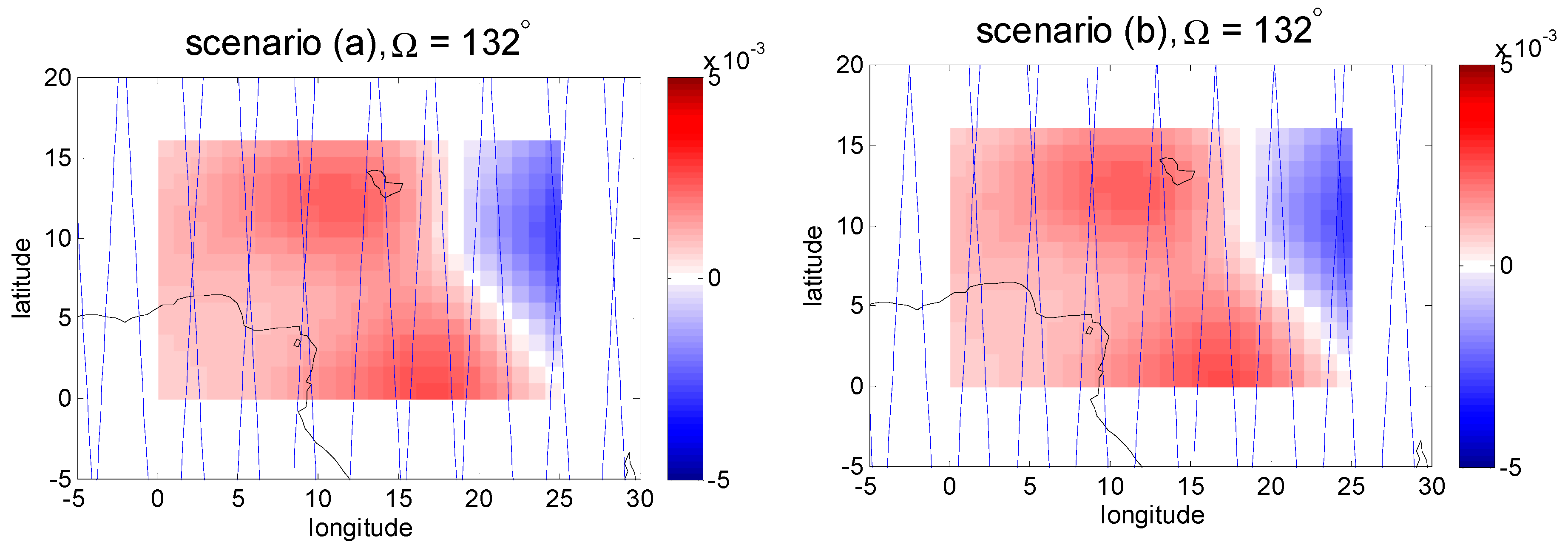
Figure 18.
Groundtrack patterns over West-Africa after 6 days. Left: Scenario (a), and right: Scenario (b). From top to bottom: Ω = 0°, 116° and 132°. The sub-cycle can be seen for Ω = 116°.
Figure 18.
Groundtrack patterns over West-Africa after 6 days. Left: Scenario (a), and right: Scenario (b). From top to bottom: Ω = 0°, 116° and 132°. The sub-cycle can be seen for Ω = 116°.


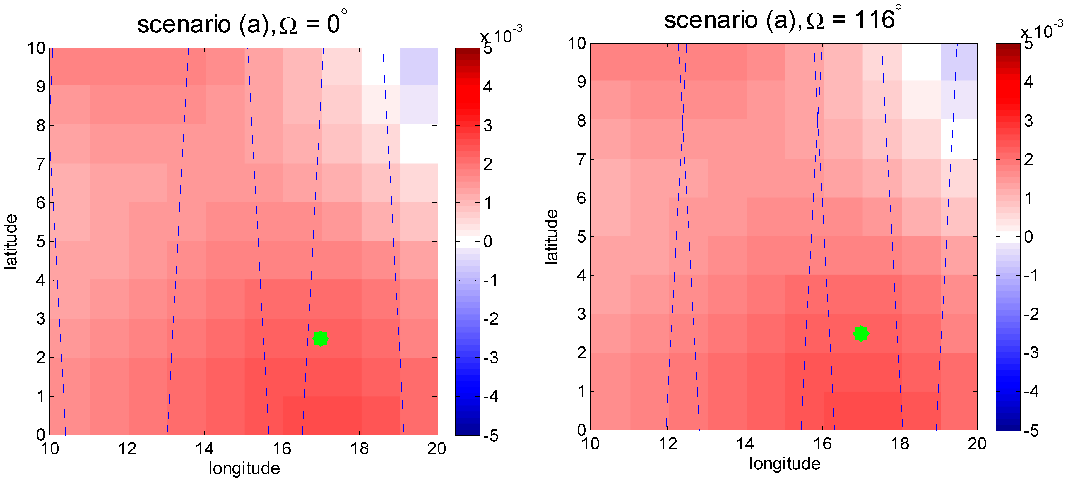
Figure 19.
Groundtrack of the scenario (a) over West-Africa for left: Ω = 0°, and right: Ω = 116° (where sub-cycle happens).
Figure 19.
Groundtrack of the scenario (a) over West-Africa for left: Ω = 0°, and right: Ω = 116° (where sub-cycle happens).

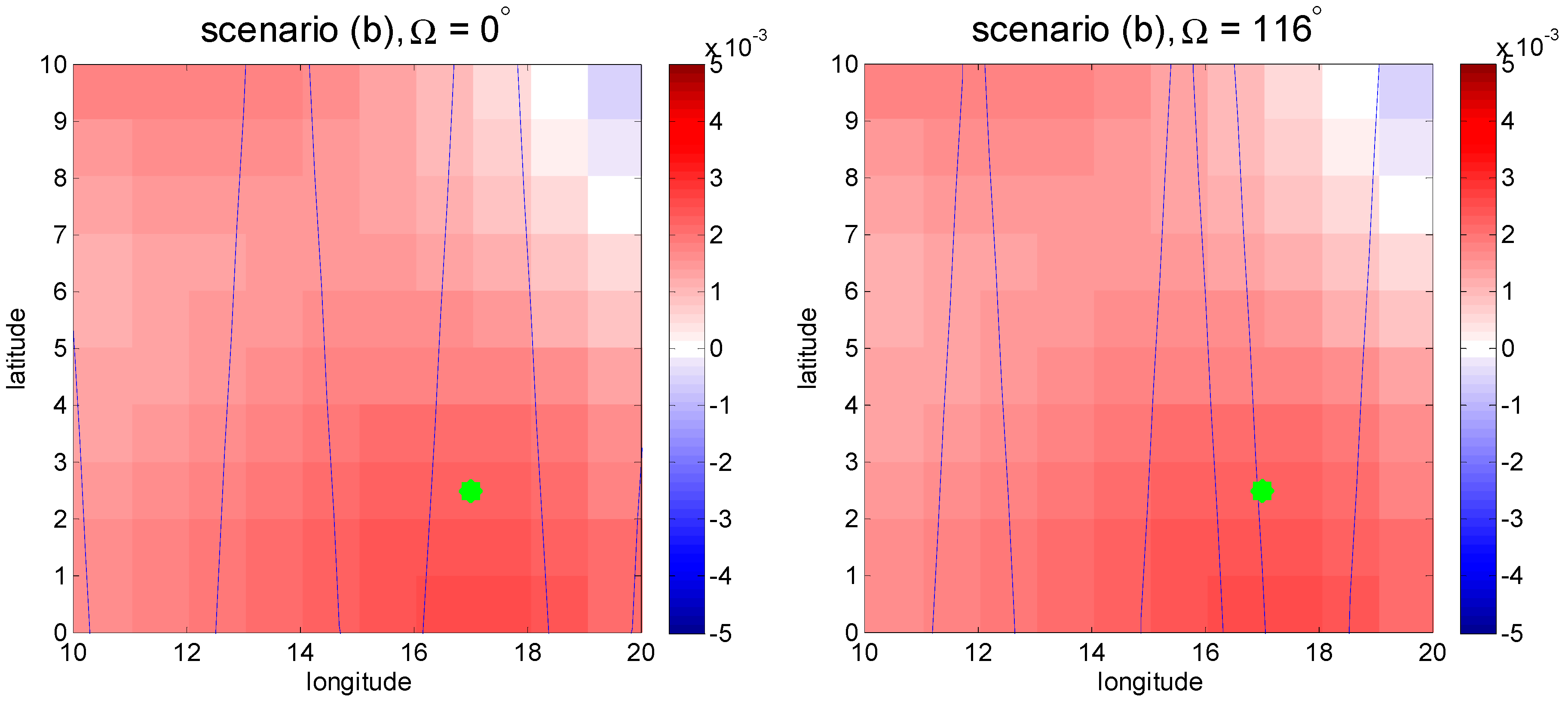
Figure 20.
Groundtrack of the scenario (b) over West-Africa for left: Ω = 0°, and right: Ω = 116° (where sub-cycle happens).
Figure 20.
Groundtrack of the scenario (b) over West-Africa for left: Ω = 0°, and right: Ω = 116° (where sub-cycle happens).

Figure 21.
Spatial covariance of a selected point in West Africa (from Figure 19 and Figure 20) for 6-day solution of the inline formation up to Lmax = 32, for top: scenario (a), and bottom: scenario (b). Left is Ω = 0° and right is Ω = 116°.

Figure 22.
Spatial covariance of a selected point in West Africa (from Figure 19 and Figure 20) for 6-day solution of the inline formation up to Lmax = 64, for top: scenario (a), and bottom: scenario (b). Left is Ω = 0° and right is Ω = 116°.

Figure 23.
Spatial covariance of a selected point in West Africa (from Figure 19 and Figure 20) for 6-day solution of the inline formation up to Lmax = CNR, for top: scenario (a), and bottom: scenario (b). Left is Ω = 0° and right is Ω = 116°.

Figure 24.
Spatial covariance of a selected point in West Africa (from Figure 19 and Figure 20) for 6-day solution of the inline formation up to Lmax = MCNR, for top: scenario (a), and bottom: scenario (b). Left is Ω = 0° and right is Ω = 116°.

Figure 25.
Spatial covariance of a selected point in West Africa (from Figure 19 and Figure 20) for 6-day solution of the Pendulum formation up to Lmax = 32, for top: scenario (a), and bottom: scenario (b). Left is Ω = 0° and right is Ω = 116°.


Figure 26.
Spatial covariance of a selected point in West Africa (from Figure 19 and Figure 20) for 6-day solution of the Pendulum formation up to Lmax = 64, for top: scenario (a), and bottom: scenario (b). Left is Ω = 0° and right is Ω = 116°.

Figure 27.
Spatial covariance of a selected point in West Africa (from Figure 19 and Figure 20) for 6-day solution of the Pendulum formation up to Lmax = CNR, for top: scenario (a), and bottom: scenario (b). Left is Ω = 0° and right is Ω = 116°.

Figure 28.
Spatial covariance of a selected point in West Africa (from Figure 19 and Figure 20) for 6-day solution of the Pendulum formation up to Lmax = MCNR, for top: scenario (a), and bottom: scenario (b). Left is Ω = 0° and right is Ω = 116°.


Table 1.
Satellite mission scenarios of this paper study.
| Scenario | β/α (ev./Day) | Altitude (km) | Sub-Cycle (Days) | Orbit Type |
|---|---|---|---|---|
| 1 | 511/32 | 263.4 | 1 | drifting |
| 2 | 509/32 | 280.8 | 11 | skipping |
| 3 | 493/31 | 281.7 | 10 | skipping |
| 4 | 206/13 | 297.6 | 6 | skipping |
| 5 | 507/32 | 298.4 | 13 | skipping |
| 6 | 95/6 | 301.3 | 1 | drifting |
| 7 | 364/23 | 303.3 | 6 | skipping |
| 8 | 205/13 | 319.4 | 4 | skipping |
| 9 | 503/32 | 333.8 | 7 | skipping |
| 10 | 485/31 | 354.9 | 14 | skipping |
| 11 | 391/25 | 356.4 | 11 | skipping |
| 12 | 125/8 | 360.7 | 3 | skipping |
Table 2.
Selected scenarios for detailed comparisons.
| Scenario | β/α(rev./Day) | Parity (β − α) | Altitude (km) | Sub-Cycle (Days) |
|---|---|---|---|---|
| a | 206/13 | odd | 297.6 | 6 |
| b | 491/31 | even | 299.8 | 6 |
Table 3.
Error RMS in terms of geoid height for global and regional (West-Africa) 6-day recovery up to Lmax = 32 of the scenario (a) inline and Pendulum formations. The smallest values in global and regional cases for each inline and Pendulum formation are written in blue.
Table 3.
Error RMS in terms of geoid height for global and regional (West-Africa) 6-day recovery up to Lmax = 32 of the scenario (a) inline and Pendulum formations. The smallest values in global and regional cases for each inline and Pendulum formation are written in blue.
| Inline (GRACE-Like) | Pendulum | |||||
|---|---|---|---|---|---|---|
| Ω = 0° | Ω = 116° | Ω = 132° | Ω = 0° | Ω = 116° | Ω = 132° | |
| Global | 3.3108 × 10⁻⁴ | 3.1546 × 10⁻⁴ | 3.1345 × 10⁻⁴ | 3.4147 × 10⁻⁴ | 2.9978 × 10⁻⁴ | 2.8446 × 10⁻⁴ |
| Regional: West-Africa | 1.5001 × 10⁻⁵ | 8.0113 × 10⁻⁶ | 1.2389 × 10⁻⁵ | 1.3820× 10⁻⁵ | 7.1328 × 10⁻⁶ | 1.2389 × 10⁻⁵ |
Table 4.
Error RMS in terms of geoid height for global and regional (West-Africa) 6-day recovery up to Lmax = 32 of the scenario (b) inline and Pendulum formation. The smallest values in global and regional cases for each inline and Pendulum formation are written in blue.
Table 4.
Error RMS in terms of geoid height for global and regional (West-Africa) 6-day recovery up to Lmax = 32 of the scenario (b) inline and Pendulum formation. The smallest values in global and regional cases for each inline and Pendulum formation are written in blue.
| Inline (GRACE-Like) | Pendulum | |||||
|---|---|---|---|---|---|---|
| Ω = 0° | Ω = 116° | Ω = 132° | Ω = 0° | Ω = 116° | Ω = 132° | |
| Global | 3.3169 × 10⁻⁴ | 3.1218 × 10⁻⁴ | 3.0947 × 10⁻⁴ | 3.3759 × 10⁻⁴ | 3.0026 × 10⁻⁴ | 2.8424 × 10⁻⁴ |
| Regional: West-Africa | 1.4774 × 10⁻⁵ | 8.3863 × 10⁻⁶ | 1.2509 × 10⁻⁵ | 1.4533 × 10⁻⁵ | 7.0561 × 10⁻⁶ | 1.2401 × 10⁻⁵ |
Table 5.
Error RMS in terms of geoid height for global and regional (West-Africa) 6-day recovery up to Lmax = 64 of the scenario (a) inline and Pendulum formations. The smallest values in global and regional cases for each inline and Pendulum formation are written in blue.
Table 5.
Error RMS in terms of geoid height for global and regional (West-Africa) 6-day recovery up to Lmax = 64 of the scenario (a) inline and Pendulum formations. The smallest values in global and regional cases for each inline and Pendulum formation are written in blue.
| Inline (GRACE-Like) | Pendulum | |||||
|---|---|---|---|---|---|---|
| Ω = 0° | Ω = 116° | Ω = 132° | Ω = 0° | Ω = 116° | Ω = 132° | |
| Global | 4.6228 × 10⁻⁴ | 4.4430 × 10⁻⁴ | 4.7008 × 10⁻⁴ | 3.5444 × 10⁻⁴ | 3.2951 × 10⁻⁴ | 3.1891 × 10⁻⁴ |
| Regional: West-Africa | 2.0185 × 10⁻⁵ | 1.6887 × 10⁻⁵ | 2.7245 × 10⁻⁵ | 1.3620 × 10⁻⁵ | 6.7006 × 10⁻⁶ | 1.2912 × 10⁻⁵ |
Table 6.
Error RMS in terms of geoid height for global and regional (West-Africa) 6-day recovery up to Lmax = 64 of the scenario (b) inline and Pendulum formations. The smallest values in global and regional cases for each inline and Pendulum formation are written in blue.
Table 6.
Error RMS in terms of geoid height for global and regional (West-Africa) 6-day recovery up to Lmax = 64 of the scenario (b) inline and Pendulum formations. The smallest values in global and regional cases for each inline and Pendulum formation are written in blue.
| Inline (GRACE-Like) | Pendulum | |||||
|---|---|---|---|---|---|---|
| Ω = 0° | Ω = 116° | Ω = 132° | Ω = 0° | Ω = 116° | Ω = 132° | |
| Global | 5.1352 × 10⁻⁵ | 4.9846 × 10⁻⁴ | 5.3826 × 10⁻⁴ | 3.5288 × 10⁻⁴ | 3.2424 × 10⁻⁴ | 3.1509 × 10⁻⁴ |
| Regional: West-Africa | 1.7985 × 10⁻⁵ | 1.6219 × 10⁻⁵ | 1.8206 × 10⁻⁵ | 1.4215 × 10⁻⁵ | 6.9308 × 10⁻⁶ | 1.3269 × 10⁻⁵ |
Table 7.
Error RMS in terms of geoid height for global and regional (West-Africa) 6-day recovery up to Lmax = CNR of the scenario (a) inline and Pendulum formations. The smallest values in global and regional cases for each inline and Pendulum formation are written in blue.
Table 7.
Error RMS in terms of geoid height for global and regional (West-Africa) 6-day recovery up to Lmax = CNR of the scenario (a) inline and Pendulum formations. The smallest values in global and regional cases for each inline and Pendulum formation are written in blue.
| Inline (GRACE-Like) | Pendulum | |||||
|---|---|---|---|---|---|---|
| Ω = 0° | Ω = 116° | Ω = 132° | Ω = 0° | Ω = 116° | Ω = 132° | |
| Global | 3.6814 × 10⁻⁴ | 3.4014 × 10⁻⁴ | 3.3387 × 10⁻⁴ | 3.4577 × 10⁻⁴ | 3.1227 × 10⁻⁴ | 2.9901 × 10⁻⁴ |
| Regional: West-Africa | 1.6740 × 10⁻⁵ | 8.7953 × 10⁻⁶ | 1.2396 × 10⁻⁵ | 1.4375 × 10⁻⁵ | 7.1110 × 10⁻⁶ | 1.3141 × 10⁻⁴ |
Table 8.
Error RMS in terms of geoid height for global and regional (West-Africa) 6-day recovery up to Lmax = CNR of the scenario (b) inline and Pendulum formations. The smallest values in global and regional cases for each inline and Pendulum formation are written in blue.
Table 8.
Error RMS in terms of geoid height for global and regional (West-Africa) 6-day recovery up to Lmax = CNR of the scenario (b) inline and Pendulum formations. The smallest values in global and regional cases for each inline and Pendulum formation are written in blue.
| Inline (GRACE-Like) | Pendulum | |||||
|---|---|---|---|---|---|---|
| Ω = 0° | Ω = 116° | Ω = 132° | Ω = 0° | Ω = 116° | Ω = 132° | |
| Global | 3.6416 × 10⁻⁴ | 3.3558 × 10⁻⁴ | 3.3128 × 10⁻⁴ | 3.4506 × 10⁻⁴ | 3.1013 × 10⁻⁴ | 2.9701 × 10⁻⁴ |
| Regional: West-Africa | 1.5778 × 10⁻⁵ | 7.5704 × 10⁻⁶ | 1.2716 × 10⁻⁵ | 1.4277 × 10⁻⁵ | 6.8994 × 10⁻⁶ | 1.3202 × 10⁻⁵ |
Table 9.
Error RMS in terms of geoid height for global and regional (West-Africa) 6-day recovery up to Lmax = MCNR of the scenario (a) inline and Pendulum formations. The smallest values in global and regional cases for each inline and Pendulum formation are written in blue.
Table 9.
Error RMS in terms of geoid height for global and regional (West-Africa) 6-day recovery up to Lmax = MCNR of the scenario (a) inline and Pendulum formations. The smallest values in global and regional cases for each inline and Pendulum formation are written in blue.
| Inline (GRACE-Like) | Pendulum | |||||
|---|---|---|---|---|---|---|
| Ω = 0° | Ω = 116° | Ω = 132° | Ω = 0° | Ω = 116° | Ω = 132° | |
| Global | 0.0418 | 0.0290 | 0.0272 | 4.2335 × 10⁻⁴ | 4.2252 × 10⁻⁴ | 3.9229 × 10⁻⁴ |
| Regional: West-Africa | 0.0067 | 3.4368 × 10⁻⁴ | 6.6340 × 10⁻⁴ | 1.5943 × 10⁻⁵ | 1.2909 × 10⁻⁵ | 1.1856 × 10⁻⁵ |
Table 10.
Error RMS in terms of geoid height for global and regional (West-Africa) 6-day recovery up to Lmax = MCNR of the scenario (b) inline and Pendulum formations. The smallest values in global and regional cases for each inline and Pendulum formation are written in blue.
Table 10.
Error RMS in terms of geoid height for global and regional (West-Africa) 6-day recovery up to Lmax = MCNR of the scenario (b) inline and Pendulum formations. The smallest values in global and regional cases for each inline and Pendulum formation are written in blue.
| Inline (GRACE-Like) | Pendulum | |||||
|---|---|---|---|---|---|---|
| Ω = 0° | Ω = 116° | Ω = 132° | Ω = 0° | Ω = 116° | Ω = 132° | |
| Global | 0.0721 | 0.0375 | 0.0646 | 4.2458 × 10⁻⁴ | 4.5364 × 10⁻⁴ | 4.0651 × 10⁻⁴ |
| Regional: West-Africa | 0.0020 | 4.2256 × 10⁻⁴ | 0.0019 | 1.8027 × 10⁻⁵ | 2.8095 × 10⁻⁵ | 1.4860 × 10⁻⁵ |
© 2018 by the authors. Licensee MDPI, Basel, Switzerland. This article is an open access article distributed under the terms and conditions of the Creative Commons Attribution (CC BY) license (http://creativecommons.org/licenses/by/4.0/).
Share and Cite
MDPI and ACS Style
Iran-Pour, S.; Weigelt, M.; Amiri-Simkooei, A.; Sneeuw, N. Impact of Groundtrack Pattern of a Single Pair Mission on the Gravity Recovery Quality. Geosciences 2018, 8, 315. https://doi.org/10.3390/geosciences8090315
AMA Style
Iran-Pour S, Weigelt M, Amiri-Simkooei A, Sneeuw N. Impact of Groundtrack Pattern of a Single Pair Mission on the Gravity Recovery Quality. Geosciences. 2018; 8(9):315. https://doi.org/10.3390/geosciences8090315
Chicago/Turabian StyleIran-Pour, Siavash, Matthias Weigelt, Alireza Amiri-Simkooei, and Nico Sneeuw. 2018. "Impact of Groundtrack Pattern of a Single Pair Mission on the Gravity Recovery Quality" Geosciences 8, no. 9: 315. https://doi.org/10.3390/geosciences8090315
Note that from the first issue of 2016, this journal uses article numbers instead of page numbers. See further details here.