Objective Regolith-Landform Mapping in a Regolith Dominated Terrain to Inform Mineral Exploration
by
 ,
,
Alicia S. Caruso
1,* ,
,
Kenneth D. Clarke
1,
Caroline J. Tiddy
2,
Steven Delean
1 and
Megan M. Lewis
1 1
School of Biological Sciences, University of Adelaide, Adelaide SA 5005, Australia
2
Future Industries Institute, University of South Australia, Mawson Lakes SA 5095, Australia
*
Author to whom correspondence should be addressed.
Geosciences 2018, 8(9), 318; https://doi.org/10.3390/geosciences8090318
Submission received: 13 July 2018
/
Revised: 10 August 2018
/
Accepted: 10 August 2018
/
Published: 24 August 2018
(This article belongs to the Special Issue Quantitative Geomorphology)
Abstract
:An objective method for generating statistically sound objective regolith-landform maps using widely accessible digital topographic and geophysical data without requiring specific regional knowledge is demonstrated and has application as a first pass tool for mineral exploration in regolith dominated terrains. This method differs from traditional regolith-landform mapping methods in that it is not subject to interpretation and bias of the mapper. This study was undertaken in a location where mineral exploration has occurred for over 20 years and traditional regolith mapping had recently been completed using a standardized subjective methodology. An unsupervised classification was performed using a Digital Elevation Model, Topographic Position Index, and airborne gamma-ray radiometrics as data inputs resulting in 30 classes that were clustered to eight groups representing regolith types. The association between objective and traditional mapping classes was tested using the ‘Mapcurves’ algorithm to determine the ‘Goodness-of-Fit’, resulting in a mean score of 26.4% between methods. This Goodness-of-Fit indicates that this objective map may be used for initial mineral exploration in regolith dominated terrains.
1. Introduction
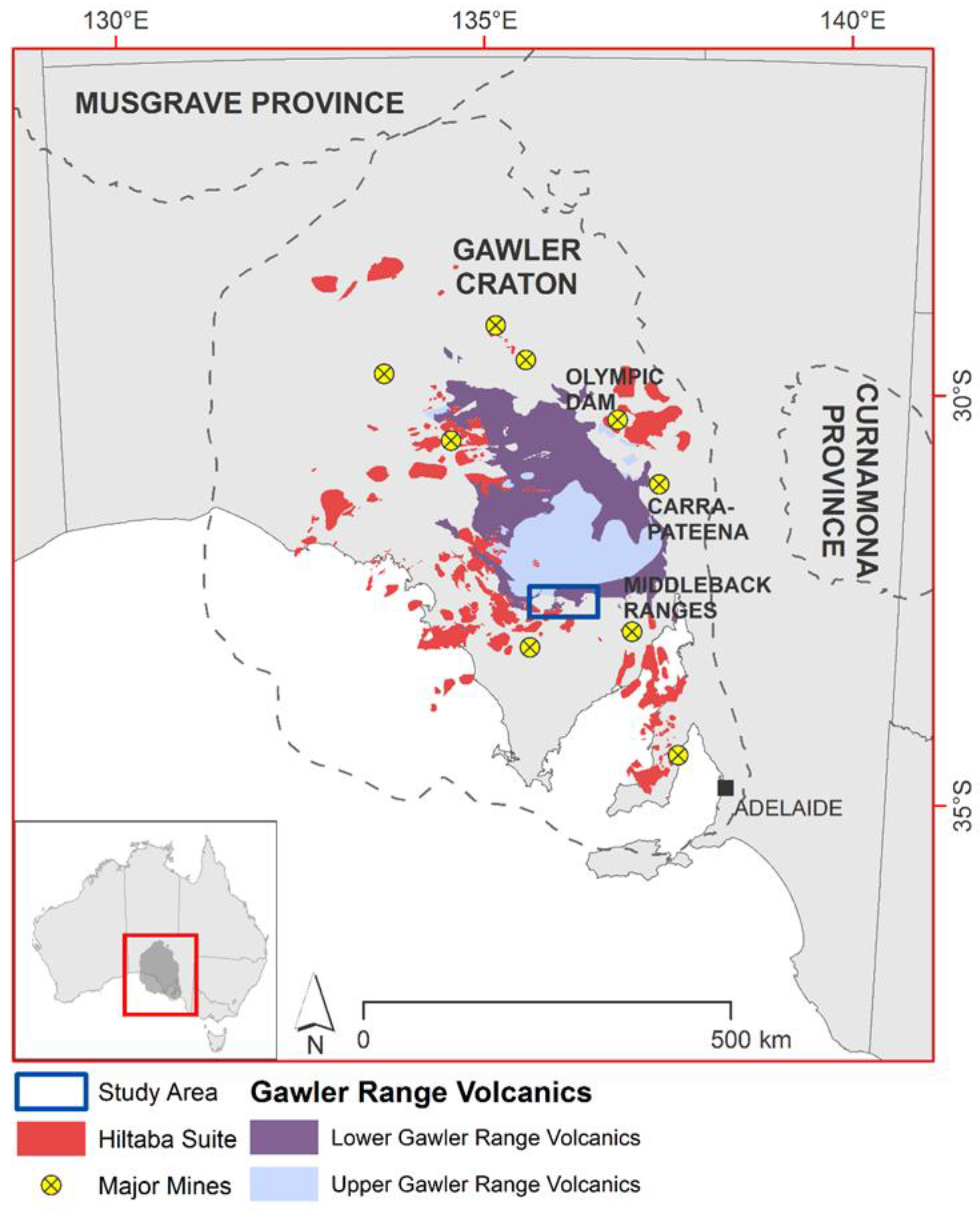
Regolith is the surface expression of the entire unconsolidated or secondarily recemented cover that overlies coherent bedrock that has been formed by weathering, erosion, transport, and/or deposition of older material [1]. Regolith is also known as the ‘Critical Zone’, the combination of chemical, geological, biological, and physical processes at the Earth’s surface preserved as sediments above bedrock [2,3]. Regolith connects to the underlying geology through weathering and commonly alters the surface expression of a buried ore body in a prospective region e.g., [4,5,6,7]. Approximately 80% of basement rocks in Australia are covered by regolith [8,9]. Given that these basement rocks are known to host numerous economically viable ore deposits of various commodities in South Australia (e.g., Olympic Dam Cu-Au-REE-U; Carrapateena Cu-Au; Middleback Ranges Fe2O3: Figure 1), they are highly prospective for mineral exploration. Therefore, regolith mapping is becoming an increasingly used tool to assist in identifying key regions for mineral exploration e.g., [10,11].
Regolith mapping contributes to understanding the geomorphology and landscape evolution of a region, but it is not a wholly objective method [5,7] and there are known spatial and compositional inconsistencies arising from differences in subjective interpretations of experts [12]. Significant progress has been made in standardizing regolith-landform mapping techniques within Australia e.g., [13,14,15]—although are subject to the preferred interpretation of the mapper. Some forms of remotely sensed data are used when creating traditional regolith-landform maps but are usually utilized as an interpretative tool [16,17]. Similarly, landform mapping has traditionally been performed through visual interpretation of aerial photography and field surveys [17,18,19]. Landforms provide an understanding of past geologic and geomorphic processes and can also be used as a surrogate for regolith mapping due to genetic and spatial links [12,20,21]. Although landforms can improve the understanding of previous processes, similar landforms can represent differing regolith domains [20]. To assist in this discrimination, the use of scale is vital as well as examining the relationship between other regolith-landform features and field validation [22].
Spatial GIS methods have evolved to enrich geomorphological maps [23] but there are few standards established for digital regolith mapping. An objective regolith map using a standard set of spatial analytical methods may therefore provide higher consistency across a region or continent [24]. The work in [4] provides an example of digital regolith mapping in a tropical environment, successfully mapping regolith and basement geology using an unsupervised classification of radiometric data and Landsat TM imagery followed by an interpretation of the weathering and geomorphic history. Integrating regolith and landforms spatially has been beneficial for mineral exploration success by identifying appropriate target regions or sampling media e.g., [12,25,26].
Recent work [27,28,29,30,31] has used a variety of machine learning methods to digitally map lithology and regolith using a range of geophysical and remote sensing data. A majority of this work has been done at regional scales, but machine learning methods have also been applied at a continental scale [32]. Although these machine learning methods have been shown to be beneficial in a range of settings, they are all advanced forms of supervised classifications. To the best of our knowledge, an unsupervised classification using geophysical and remote sensing data has not been used to produce a useful regolith-landform map in Australia.
In this paper, we create an objective mapping method to map broad regolith-landforms based on readily available digital landform and gamma-ray spectrometry data. The example is from the southern Gawler Ranges in South Australia, which is host to several prospective targets including the Paris silver deposit and the Nankivel porphyry copper prospect (Figure 1). We present and discuss a statistical comparison between the newly proposed objective mapping method and traditional regolith-landform mapping followed by the examination of this application of this technique to mineral exploration.
2. Background
2.1. Geological Setting
The area used in this study covers 3866 km2 within the southern region of the Gawler Craton (Figure 1) and includes a variety of landscape and vegetation features. The study area includes the ‘Gawler’ region and ‘Gawler volcanics’ and ‘Myall Plains’ sub-regions of the Interim Biogeographic Regionalisation for Australia (IBRA) [33]. The landscape is broadly characterized by hills, hill foot slopes, and sandy plains [34]. The vegetation varies across the sub-regions but mainly comprises low open woodlands of Western Myall (Acacia papyrocarpa) and Black Oak (Casuarina pauper) trees over sparse shrub understoreys of Bluebush (Maireana spp.), Saltbush (Atriplex spp.), and Spinifex (Triodia spp.).
The oldest basement rocks are preserved in the south of the study area and are poorly exposed. These rocks are part of the Sleaford Complex (ca. 2550–2440 Ma) and the unconformably overlying Palaeoproterozoic Hutchinson Group [35,36,37]. The Warrow Quartzite is the oldest unit of the Hutchinson Group within the study area and has an age of ca. 2008 Ma [38,39]. The Gawler Range Volcanics (GRV) are well exposed in the north of the study area and variably exposed throughout the southern and central thirds of the study area. Within the study area, the GRV is defined as the Lower GRV (Figure 1) which has an extrusion age of ca. 1591–1588 Ma [40]. The Hiltaba Suite is co-magmatic to the GRV but has a longer extrusion time of ca. 1598–1574 Ma [39,41]. It occurs widely throughout the Gawler Craton and is known to be associated with the major tectonothermal and metallogenic episode that impacted much of the Gawler Craton e.g., [35,37] (Figure 1).
The composition and formation of the regolith in the study area is described in detail by [42]. Archean and Palaeoproterozoic basement rocks are uncomfortably overlain by much younger Cenozoic sediments. Limited regolith was deposited throughout the Paleogene and Neogene, and mostly comprises ferricrete, silcrete, some colluvial sediments, and palaeochannel sediments of the Garford Formation. The Garford Formation occurs in low relief areas and includes carbonaceous clay and silt with other fluvial and lacustrine sediments.
Development of ferricrete and silcrete continued into the Quaternary, cementing host lithologies and fragments of quartz and other material. A variety of sediments were deposited including aeolian, terrestrial, colluvial, and lacustrine. Colluvial sediments comprise ferruginous and poorly sorted pebbly conglomerate and sandstone. Calcrete formed throughout the Quaternary as laminated sheets of nodular aggregates now generally exposed in erosional terrains near alluvial channels and in areas of deflation. During the Pleistocene, aeolian sediments dominated and are characterized by fine to medium grained sands, some of which formed ridges and swales. The most recent sediments deposited were aeolian quartzose sands draped over lacustrine and other aeolian deposits on the leeward side of playas [42].
2.2. Regolith Mapping
A regolith unit is a subdivision of the regolith with visibly distinguishable boundaries at a mappable scale. The term can also be used for zones or horizons of weathering profiles [1]. There are many ways regolith unit are classified but the most common schemes are TI (Transported or In-situ) or RED (Relict, Erosional, or Depositional) [11,44]. Following this classification, the units may be categorized according to sediment origin e.g., marine or terrestrial. Then units may be distinguished based on physical attributes such as grain size, thickness, composition, to create detailed descriptions. If possible, age will also be included in the definition to provide an understanding of landscape formation processes that occurred in the region. Some units also include information on predominant vegetation cover.
Traditional regolith mapping of the Yardea and Port Augusta 1:250,000 map sheets was completed in 2016 by [42], and the study area for this work is a small section of this mapping area where there are known exploration targets. The original mapping involved a combination of visual interpretation and some field assessment of a number of available data sets including: state geological mapping, Landsat TM5 and ETM7 imagery, 1 and 3 s Digital Elevation Models (DEMs), and gamma-ray radiometric data [45]. Ten attributes were assigned to mapping units including regolith materials, landform names, Regolith Terrain Map (RTMAP) code, and TI scheme. Bedrock weathering intensity and regolith thickness were not able to be inferred from the data used but are available as individual products from the Geological Survey of South Australia. The final product was based on the 1:100,000 geology mapping using the RTMAP scheme developed by [14].
3. Materials and Methods
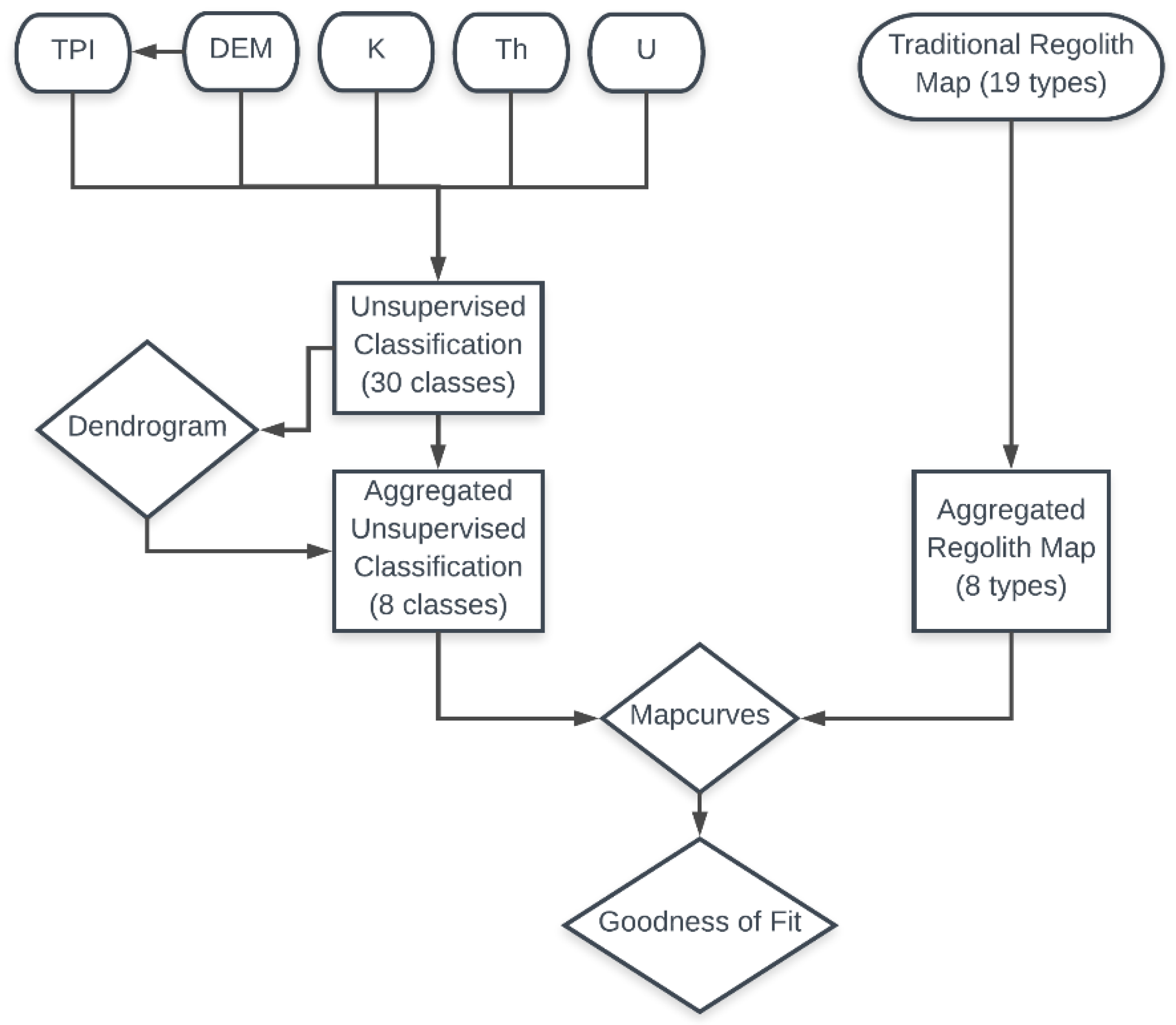
The methods for this work were multi-faceted and are detailed in the following subsections with an overview presented in Figure 2.
3.1. Clustering of Traditional Regolith Map
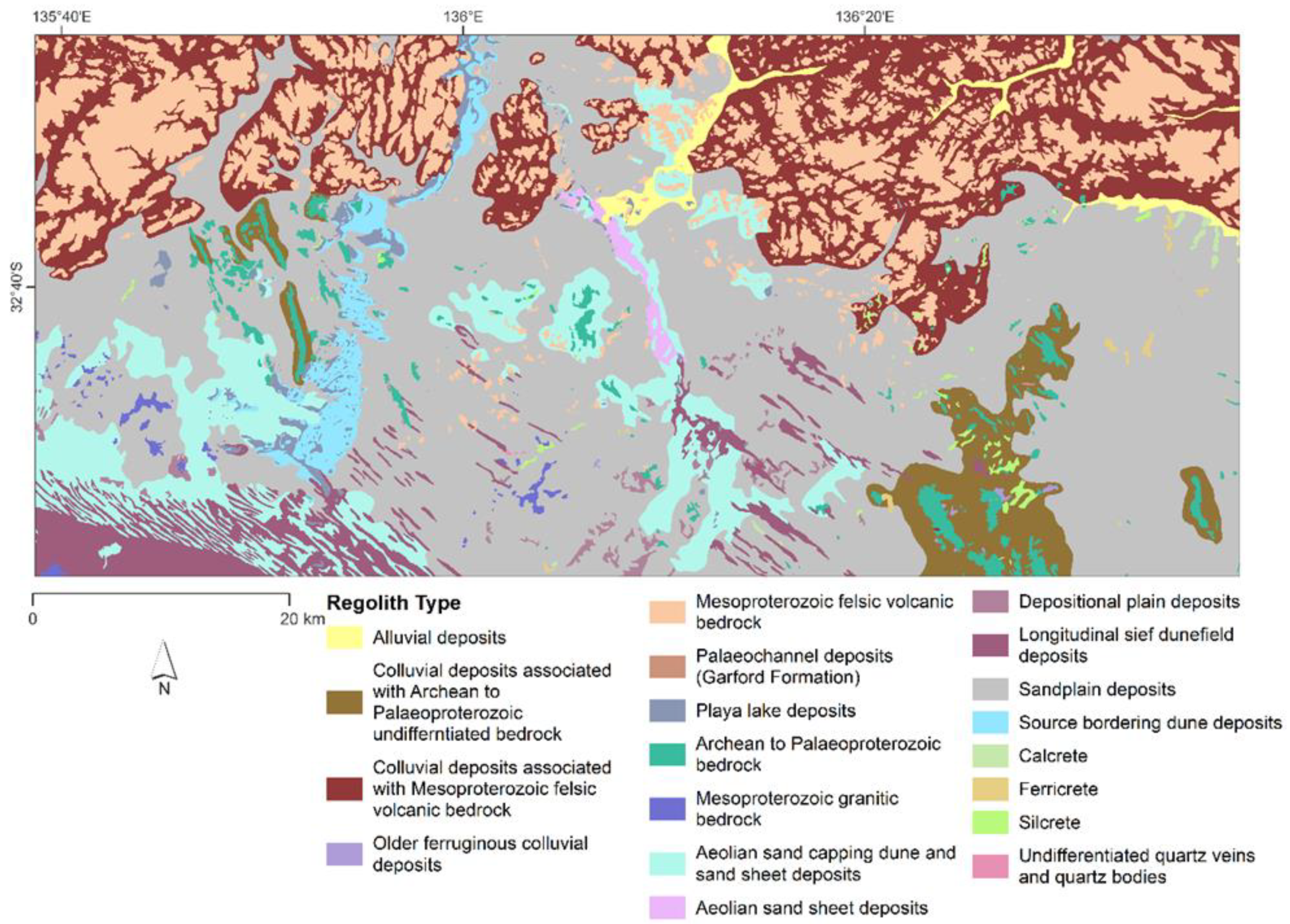
Figure 3 shows the regolith map of [42] for the study area. This map shows 19 regolith-landform units that depict the fine scale detail throughout the map area. The landscape is clearly dominated by a few regolith types with a majority of others sparsely distributed and limited in extent (Figure 3). Due to the limited extent of some regolith units, the 19 regolith map units were aggregated into eight types based on their spatial distribution and description of regolith material origin. The topological integrity of the mapping was retained although the number of overall regolith classes was reduced. An example of this was aggregating silcrete, calcrete, and ferricrete together (Duricrusts) to retain topology as they are expressed with the same landform at surface. Similarly, the palaeochannel deposits and playa lake deposits were also spatially limited and were clustered together to preserve map topology and include these regolith types as an exclusive class, water related formation processes (Lake/Palaeochannel sediments, Table 1). The accuracy of the DEM methodology that is applied in this work does not allow to discriminate them.
Although this aggregation retained some types of regolith, others were clustered to provide greater clarity. For example, the Sandplains/dunes, mostly aeolian origin regolith type (herein referred to as ‘Sandplains/dunes’) includes sediments formed by wind formation processes, longitudinal sief dune field deposits and aeolian sand sheet deposits (Table 1). Colluvial sediments occurring in the north and south of the study area were clustered together as they are derived from the same formation processes (erosion–weathering–transport–deposition sediments).
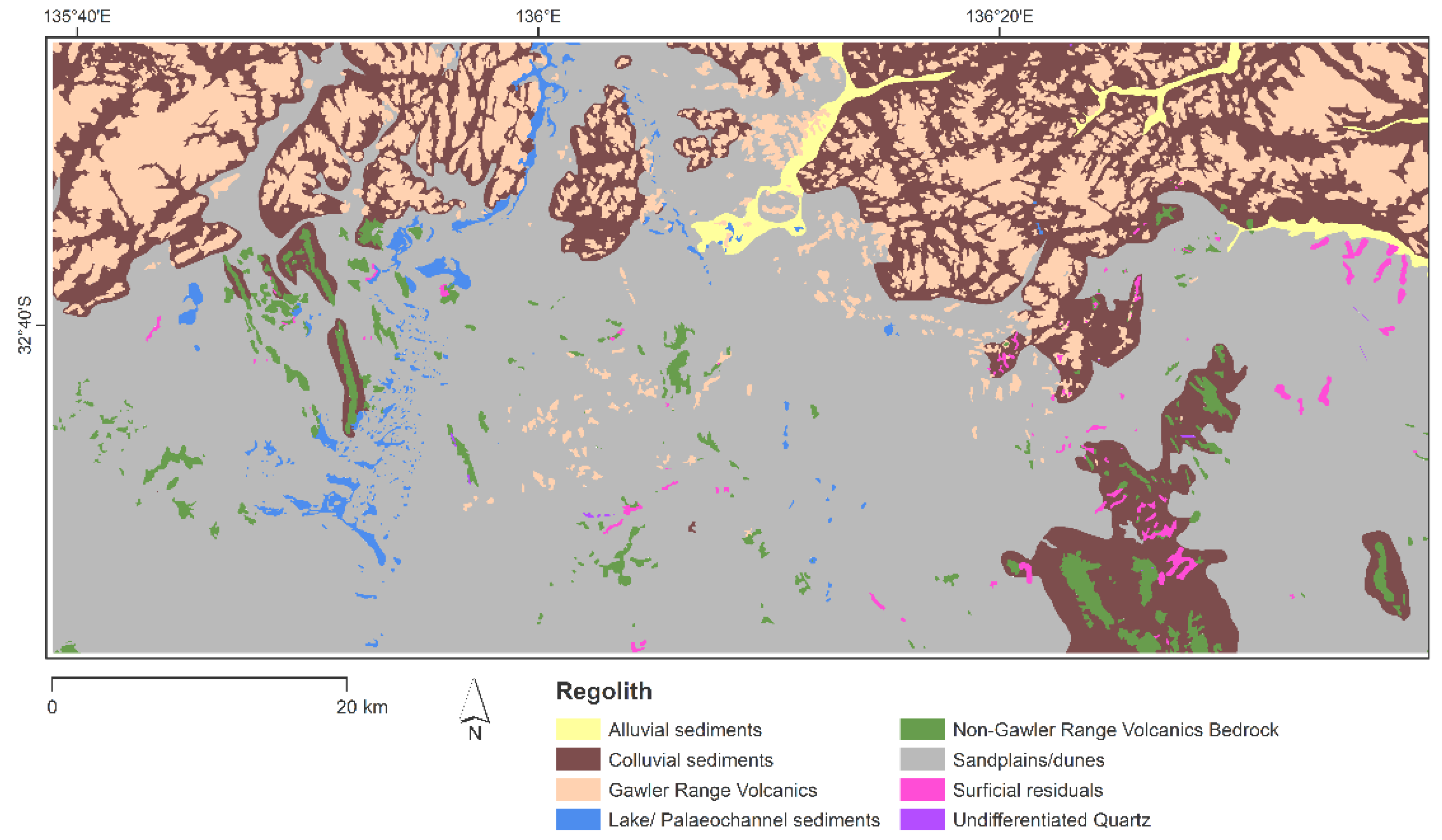
Some regolith types were particularly distinctive and were not aggregated in the Clustered Regolith Mapping Unit (CRMU) map (Figure 4) as they were considered to be unrelated to other regolith types. These included Alluvial sediments, GRV bedrock, and Undifferentiated Quartz. It is known that GRV and Non-GRV bedrock are compositionally different [35,46] and undergo differing formation processes, therefore it was reasonable to keep these regolith types separate in the clustering process (Figure 4, Table 1).
Table 1 shows the clustering of the original 19 regolith types of [42] to form the CRMU map shown in Figure 4. The reduction of detail in the CRMU map has simplified regolith primarily in the southern two-thirds of the study area (Figure 4). Clustering the traditional regolith map based on formation processes alone can introduce some bias and subjectivity in this method.
3.2. Regolith-Landform Analysis
The data used to perform the regolith-landform analysis was selected for its comprehensive extent and high spatial resolution. This data is also of high quality for this remote region of South Australia. All data and data transformations used in this work are freely available, produced by Geoscience Australia and cover the entirety or vast majority of Australia providing the ability to replicate this method.
3.2.1. Spatial Data and Transforms
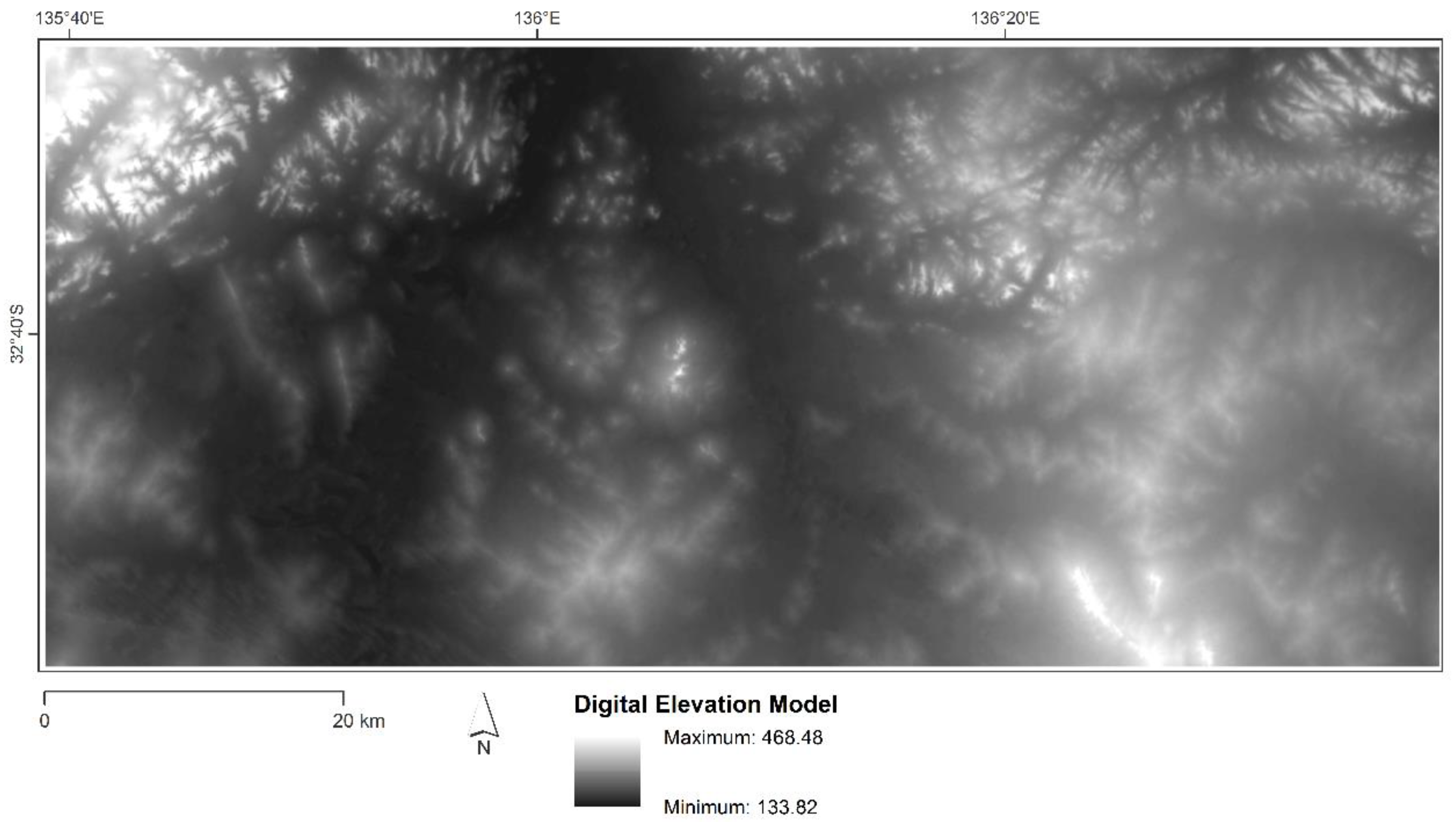
Spatial data used in the analysis includes a Digital Elevation Model (DEM), Topographic Position Index (TPI), and Slope Position Classification (SPC) derived from the smoothed DEM (DEM-S) derived by Geoscience Australia from the 1-second Shuttle Radar Topography Mission (SRTM) of NASA in 2000 with a spatial resolution of 30 m [47] (Figure 5).
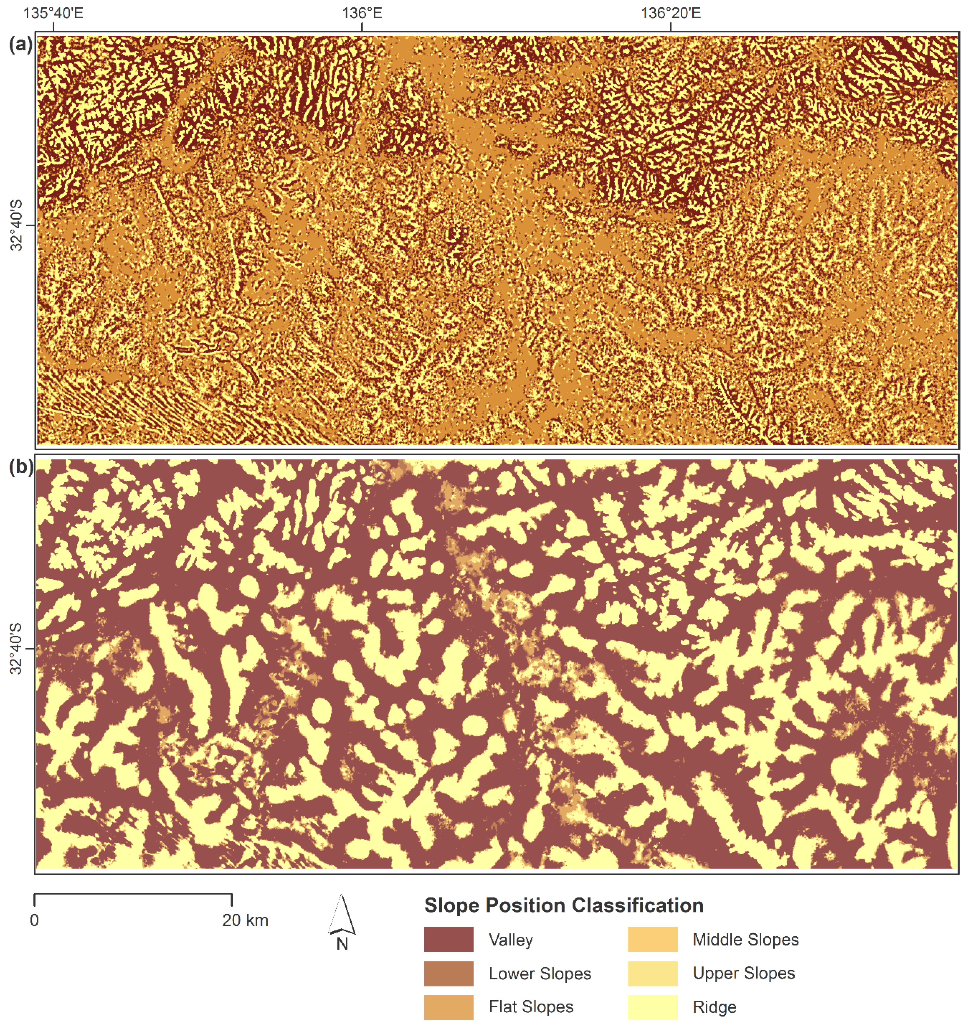
The TPI developed by [48,49] has been used to interpret numerous landscapes globally and across disciplines e.g., [50,51]. TPI is calculated as the mean elevation within a focal window of a specified radius around each cell in a DEM [48]. This index is scale dependent, with fine scales more appropriate for exploring soil erosion and coarse scales appropriate for studying regional landforms. The study area was analyzed at a coarse (2000 m radius) and fine (300 m radius) scale using ArcGIS 10.3 Toolbox [52].
The TPI is an index of curvature and while mathematically meaningful is not easily interpreted. However, the SPC classifies this index into a more interpretable form that describes the slopes in the study area. SPC is not a geometric classification of a landscape, it uses the local elevation and slope conditions for each point based on the TPI using standard deviation thresholds listed in Table 2, as defined by [48]. These thresholds are appropriate across different terrains, as shown by [51,53]. The SPC algorithm applied to both TPI grids to visualize the landscape patterns at the different scales (Figure 6).
3.2.2. Gamma-Ray Radiometrics
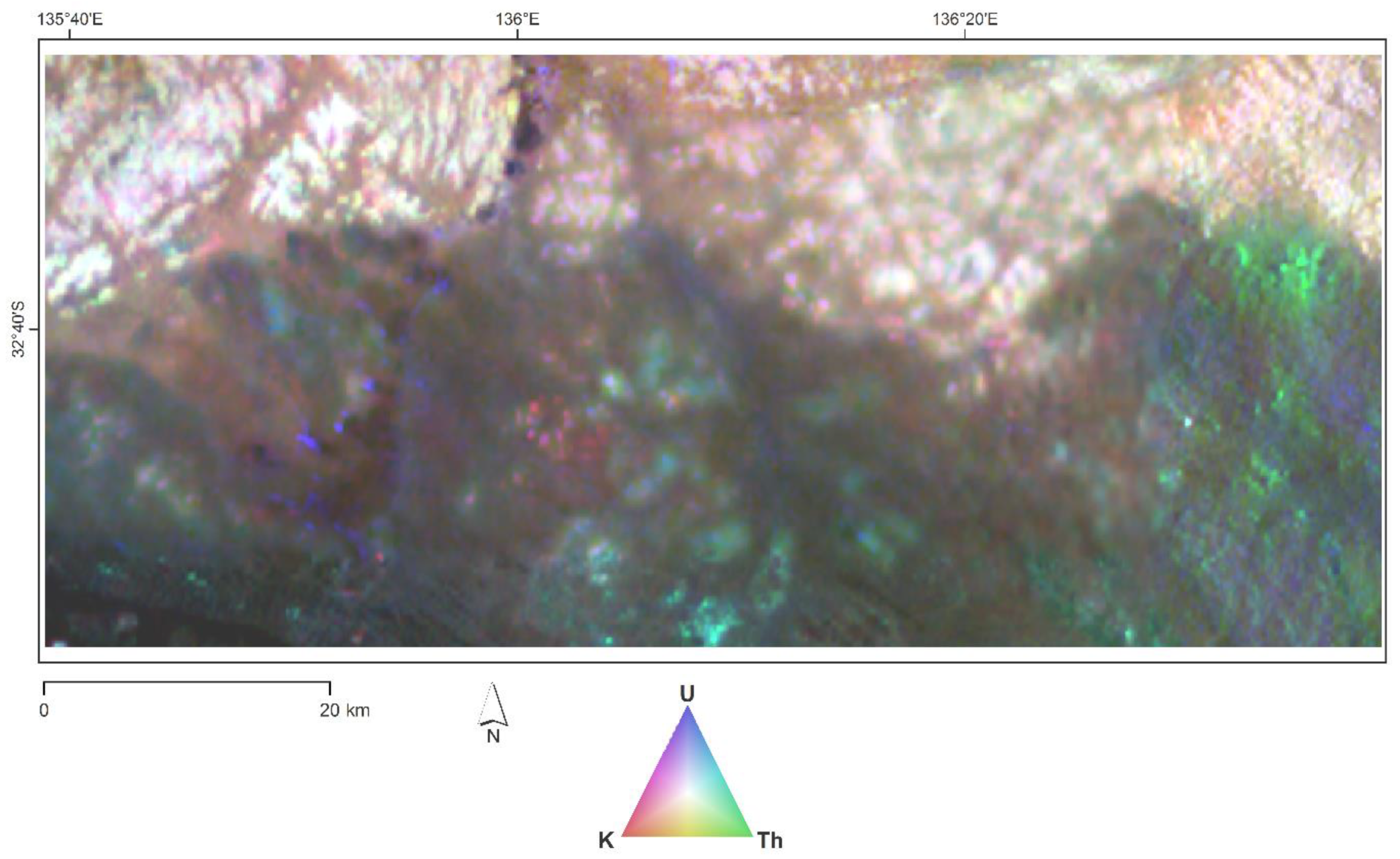
Digital maps of potassium, thorium, and uranium emissions were obtained through the South Australian Resources Information Gateway (SARIG: https://map.sarig.sa.gov.au/) with a spatial resolution of 100 m (Figure 7). The data were derived through interpolating data of previously flown airborne radiometric surveys based on methods from the Australia Wide Airborne Geophysical Survey [54,55].
3.3. Unsupervised Classification
An unsupervised classification was used to cluster and identify spatial patterns in the input data sets. Inputs for the unsupervised classification were elevation from the DEM; two TPIs of different radii (2000 m and 300 m); and gamma-ray radiometric grids for potassium, equivalent thorium, and equivalent uranium (Figure 5, Figure 6 and Figure 7). An Iso Cluster Unsupervised Classification was performed classifying the gridded data into 30 classes. These were clustered to eight classes using a class similarity threshold applied to a dendrogram of between-class distance of sequentially merged classes. This threshold was informed by visual interpretations of the spatial distribution and coherence of the classes produced.
3.4. Relationship between Mapping Methods
The relationship between the aggregated unsupervised classification and the CRMU map classes was evaluated using the Mapcurves ‘Goodness-of-Fit’ (GOF) measure developed by [56]. This measure evaluates the spatial concordance between the two maps (Equation (1)).
where A is the total area of the category on the compared map, B is the total area of the category on a reference map, and C is the amount of intersection of a category between two maps.
This method was selected because of its ability to be applied to maps with differing numbers of categories and as it is independent of resolution [56,57]. Mapcurves analysis has been successfully used to compare categorical maps in a variety of disciplines including species distribution and biogeographical region modelling e.g., [58,59]. Mapcurves analysis was implemented using 5000 points generated randomly across the study area. For each of these points, the mapped class and regolith type was sampled for each mapping method. The Mapcurves implementation of [60] was applied using 400 iterations of the algorithm using a random subsample of 500 of the 5000 points. Finally, we considered the sensitivity of the statistics from the 400 Mapcurves outputs.
4. Results
4.1. Aggregation of Traditional Regolith-Landform Map
With the number of regolith mapping units of the traditional regolith map reduced to eight, it becomes much easier to visualize the distribution of broad regolith types. Figure 4 shows that the landscape is dominated by Sandplains/dunes and the Gawler Range Volcanics in the north of the study area. The landscape also contains a large proportion of Colluvial sediments, generally surrounding bedrock, mostly around the Gawler Range Volcanics in the north of the study area. Figure 4 also highlights the prevalence of Non-Gawler Range Volcanics bedrock in the south and western regions of the study area. There are smaller units of Duricrusts and Lake/Palaeochannel sediments across the study area. Duricrusts mostly occur in the eastern portion of the study area, and are in proximity of Colluvial sediments and Non-GRV bedrock. Alluvial sediments appear as they did in Figure 3, as they were not aggregated with other regolith types.
4.2. Aggregated Unsupervised Classification
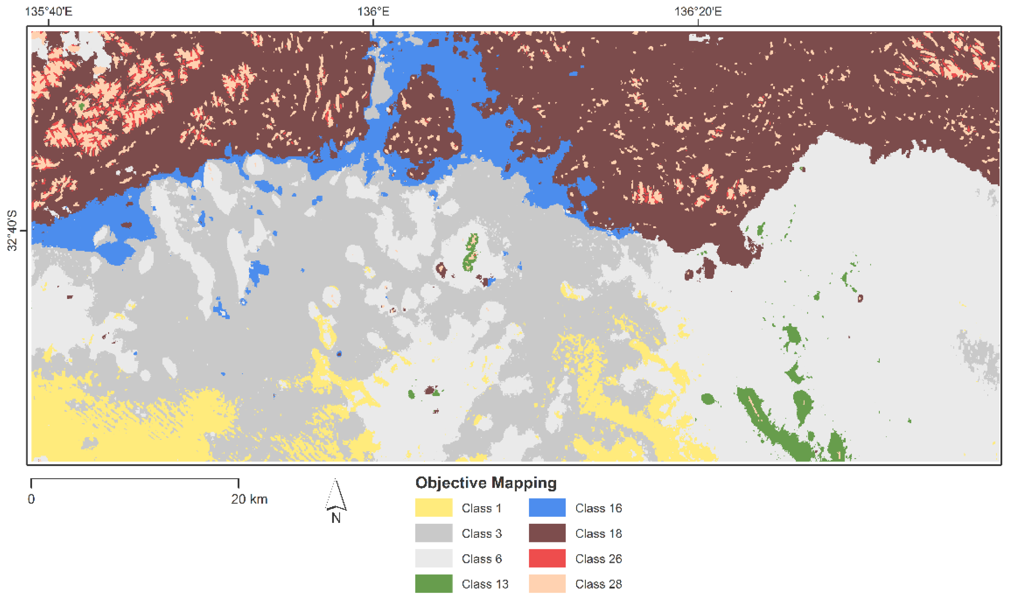
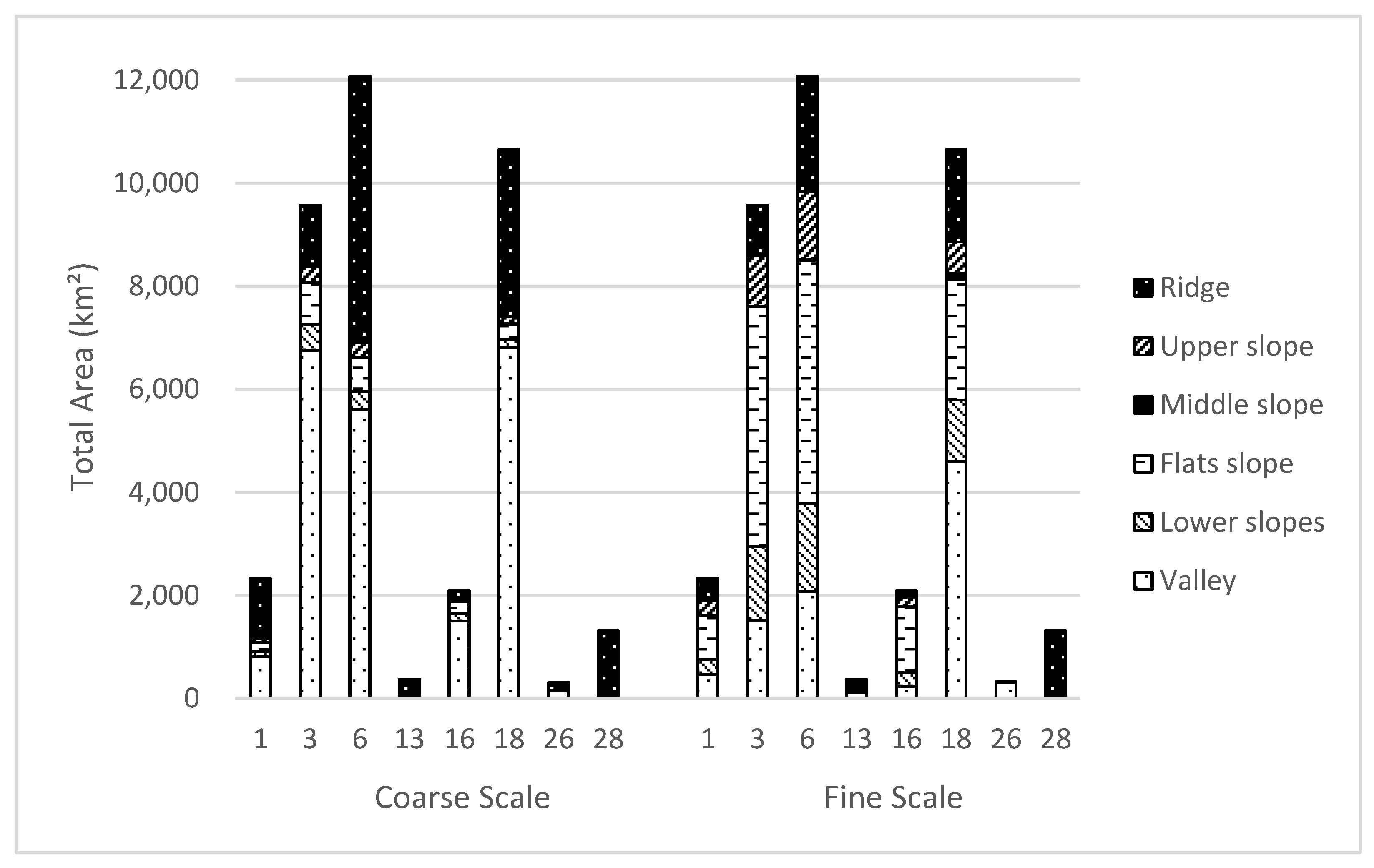
The unsupervised classification produced 30 classes which were clustered hierarchically into eight broad groups. Figure 8 shows the aggregation of the classes, indicating the threshold used to establish the aggregated unsupervised objective mapping (herein referred to as ‘the image map’) classes displayed in Figure 9. Table 3 displays the average values of input variables for each derived class with the average crustal abundances of radiometric variables included for comparison. The distribution of Slope Position Classes, both coarse and fine scale for each mapping class are shown in Figure 10.
4.3. Composition and Distribution of the Image Mapping Classes
Class 3 accounts for 24.7% of the study area. It is mostly located across the western-central region of the study area with some small areas located in the far east and north. The raw radiometric data (Figure 7) indicates that this region is rich in thorium, confirmed in Table 3 with approximately average crustal abundance values for thorium and below average abundances for potassium and uranium. At the coarse SPC analysis, this class is predominately made up of valley features; whereas at the fine scale, a higher proportion of flat slopes and upper and lower slopes are evident.
Class 1 is distributed in the south east and across some of the southern margin of the study area and makes up 6% of the study area. It has an average elevation of 202 m, with below-average abundance of all radiometric elements. At the coarse scale of topographic analysis, this class comprises mostly ridge features with 35% valley features (Figure 10). At the fine scale, much of this is identified as flat slopes, accounting for 36% of the terrain.
Class 6 is the largest class, making up 31.2% of the study area but more commonly in the east. This class has an average elevation of 250 m with some enrichment in thorium and uranium. This class has above-average abundance of thorium but below-average values of potassium and uranium. Class 6 contains approximately half ridge and half valley features at the coarse scale with the fine scale illustrating upper, flat, and lower slopes forming 64% of this class.
Class 13 is the most geographically restricted class at <1% of the total area, confined to high ridges in the southern and central regions. This class contains the highest mean elevation at 346 m above average thorium and approximately half the average abundance of potassium and uranium. The coarse SPC shows this class has 95% ridge features but 45% ridge features combined with valley and other slope features at the fine scale.
Class 16 is restricted to the north and the southern boundary of class 18 in the west of the study area. This class contains the lowest average elevation at 165 m. Figure 7 suggests that this class would be high in uranium, but the abundance in Table 3 indicates that this class contains 1.81 ppm, below average. Thorium and potassium are both above average crustal abundance. Valley features make up over 70% of the coarse SPC, whereas the fine scale indicates contains a higher occurrence of flat slopes at 61%.
Class 18 is the second largest class derived, making up 27.5% of the study area. It is mostly located in the central to western region of the study area with some small areas located in the north. Figure 7 indicates that this class is high in all three radiometric elements and Table 3 attests that this class contains average or clearly above average abundances. The coarse scale highlights the large proportion of valley features for this class with approximately 30% ridge features. At the fine scale, intermediate slope types make up a large proportion of the SPC result and ridge and valley features are reduced in their proportion.
Class 26 is the smallest of all classes at 0.85% of the area and it is spatially restricted, likely due to its representation of specific landscape features. It contains above-average radiometric values across all elements with all three elements, with potassium and uranium being the greatest of all classes. The coarse scale indicates an approximately equal division between ridge and valley features whereas the fine scale clearly shows the high proportion of valley features within this class. This class also has one of the highest average elevations of all classes at 293 m.
Class 28 makes up 3.4% of the total area and is distributed across the northern region with exceptions in the central and southern margins. This class has the second-highest average elevation at 306 m with Figure 7 and Table 3 in agreement that this class is high in all three radiometric elements. This class is represented by primarily ridge features at the coarse and fine scale. Class 28 illustrates the most dominant relationship with one slope type compared to all other classes identified in the final mapping method.
Classes 13, 16, and 26 were not aggregated with other classes and are noticeably distinct (Figure 8, Table 3). Class 1 is a relatively unique class as it is formed from two classes during aggregation but has some similarity to Classes 3 and 6 in the thorium and uranium content. Coincidentally, Classes 1, 3, and 6 are adjacent across the southern two-thirds of the study area (Figure 9).
4.4. Spatial Concordance between Mapping Methods
The iterative Mapcurves function produced Goodness-of-Fit (GOF) scores between map classes ranging from 22.4–38.5% with a mean GOF of 26.4%. Table 4 shows the mean GOF for each intersection between the CRMU and the image mapping classes, indicating the highest GOF scores for each image mapping class. The intersection of Class 3 and Sandplains/dunes has the largest GOF score at 35.98%, followed by Class 18 and Colluvial sediments at 31.8%. Other large GOF scores also occur between Class 28 and 18 and Gawler Range Volcanics and Class 13 and Non-Gawler Range Volcanics CRMU regolith types.
When comparing the image map to the CRMU map, Classes 1, 3, 6, and 16 have the highest GOF with Sandplains/dunes. The Gawler Range Volcanics CRMU regolith type has multiple correspondences with Classes 26 and 28. None of the 5000 randomly generated points fell within the Undifferentiated Quartz regolith type due to its small area, therefore it was not included in the Mapcurves analysis.
5. Discussion
5.1. Relationship between Maps and Input Variables
Sandplains/dunes has two large GOF scores with Classes 3 and 6 at 35.98% and 30.41% respectively. When examining Figure 9 in conjunction with Table 4, it can be seen that Classes 3 and 6 make up a majority of the central region of the study area. Comparison with Figure 4 demonstrates that both classes have high GOF scores with this CRMU regolith type due to the majority of the CRMU map comprising Sandplains/dunes with other regolith types scattered throughout the central region of the study area. The image map shows two different classes (Classes 3 and 6) that make up approximately the same area (Figure 9). It is likely that this is due to elevation and SPC input data. It can be seen in Figure 5 that an area of high elevation on the eastern side and centre of the study area, corresponds with Sandplains/dunes in Figure 4. From Table 3, elevation and radiometric thorium content will likely explain the separation of Classes 3 and 6 and hence their similar GOF scores.
Although there are strong relationships between Sandplains/dunes and Classes 3 and 6, there are much smaller GOF scores with this CRMU regolith type and Classes 1 and 16 (Table 4). Figure 4 shows that the south western corner and central northern portion of the study area are sandplains/dunes but these have been separated in the image mapping as Classes 1 and 16 respectively likely due to the differences in both radiometric response and elevation from Figure 4 and Figure 6 and Table 3. This means that Classes 1 and 16 are not as well predicted from Sandplains/dunes and they make up a smaller proportion of this CRMU regolith type, explaining their low GOF scores.
Class 18 has strong correspondence with both Colluvial sediments and the Gawler Range Volcanics (Table 4). The northern regolith types are distinct in the radiometric input data (Figure 7) as they are high in all radiometric elements, confirmed in Table 3. Figure 4 shows the extent of the GRV in the north of the study area and when comparing this to Figure 9, it can be seen that Class 28 is not as extensive. The strong similarities of the radiometric responses explain the separation of classes and therefore high GOF scores for both Colluvial sediments and GRV with Class 18.
While there are areas of higher GOF, there are also many minor GOF values which still indicate some relationship between map classes (Table 4). The GOF between Colluvial sediments and Class 6 at 3.57% is due to the aggregation of the unsupervised classification. Class 6 includes some Colluvial sediments in the eastern half of the study area when comparing Figure 3 and Figure 8. This type of interaction between mapping methods also occurs with Class 18 and Alluvial sediments.
5.2. Mapcurves for Comparison of Regolith-Landform Maps
The choice of map to use as the reference is subjective and will produce differing outcomes. Mapcurves analysis permits the comparison of mapping methods to be made in both directions, i.e., using the traditional map or the image map as the reference for the comparison between classes. The comparison that produces the greatest GOF is considered to be the best direction of concordance between the maps and may also indicate which map is finer scale [56]. It has been suggested by [63] that the coarser map would be advantaged when selecting the highest Mapcurve result. However, given the similarity in scales of the two maps compared in this study this seems unlikely to be an influencing factor in the results.
The Mapcurves result suggests that in this case the traditional map should be used as the reference as the greatest GOF score (26.4%) is for the comparison of the image map to the traditional map. This Goodness-of-Fit indicates that our objective regolith-landform map describes some of the same pattern as the traditional subjective map, but also contains significant additional information, probably resulting from the topographic indices and radiometric data. An unsupervised regolith-landform map is easily evaluated using Mapcurves as shown in this study. Mapcurves can provide confidence in this mapping method due to its numerous advantages, such as application beyond a pair-wise comparison with multiple maps and resolution independence. This work has identified, analyzed, and interpreted the GOF scores and intersections between classes (Table 4) to bring greater interpretation to the objective regolith-landform map and how it relates to the traditional map.
5.3. Regolith-Landform Mapping without Prior Knowledge
The generation of an objective map from digital data that is comparable to the pre-existing regolith-landform map demonstrates that it is not necessary to have extensive knowledge of a site prior to using this method. This is because the image map is data driven and the methodology identifies meaningful patterns in the data. The characteristics of the image mapping classes have been derived from summary measures of the input variables. When used as a first-pass analysis tool, the objective mapping method can provide a basis for targeted field work to further describe and characterize regolith units.
Although most classifications of landforms are attempting to replicate a manual classification [64], an objective method that provides similarities to a traditional map does have its place. In this case, the objective mapping method illustrates the effectiveness of using easily and freely accessible data and simple methodology. The image mapping could also be accomplished on open source software such as QGis. It can be argued that this method is faster, taking only days versus weeks of field work followed by quality control, meaning turnaround time of a regional regolith-landform product is reduced and that publication of products to be used in a number of applications, such as mineral exploration, are more accessible.
While this method results in faster production of regolith-landform maps, it is not intended to be a replacement for ‘boots on ground’ mapping. The objective mapping method presented here gives an indication of the distribution of broad scale regolith-landform features. Therefore, if the traditional mapping method were to be discarded detailed descriptions and interpretations of regolith and soil types would be lost. This highlights why ‘boots on ground’ mapping and regolith expertise will always be useful and could be incorporated into a data-driven methodology. Other research comparable to this study primarily focused on providing descriptive attributes for each defined class rather than an overview and statistical measure of fit e.g., [19,65,66]. Supervised classification methods, including machine learning methods such as fuzzy k-means or Self-Organizing Maps, provide continuity between classes and are described as more of a continuous classification method [24,32,67]. However, they require training data or an accuracy assessment to verify their resulting product unlike this study which used a statistical measure to evaluate the objective method.
The relationships between the image map classes and regolith types mapped by traditional methods for the southern Gawler Ranges study area demonstrates that this mapping method based on digital data analysis could be implemented in other regolith dominated terrains. In regions of sporadic or no coverage of regolith mapping, this method could be used prior to a field campaign to gain insight and understanding of the landscape without the time or expense required for traditional mapping. Digital data including geology and high-resolution satellite imagery that provide insights to alternative landform features are example avenues that could be considered as additional input datasets.
5.4. Application for Mineral Exploration
Objective mapping methods can be beneficial in expanding geological understanding prior to entering an area for purposes such as mineral exploration. As knowledge of the geomorphology and landscape is improved with mapping, exploration models can be adapted to be better suited for the environment of the explorer [68]. The extensive, and in places very deep, sedimentary cover across regions such as the Gawler Craton can be a huge barrier to explorers considering exploration targets. This method could assist in identifying a specific regolith-landform type and identifying areas of rock exposure with negligible time and monetary expense.
It is advantageous to integrate both regolith and landforms to enhance possible geochemical exploration success by identifying appropriate sampling media once a regolith-landform map has been produced [12,25,26]. For some initial geochemical soil sampling, this image mapping could provide an intuitive guide to the regolith-landform characteristics and highlight where sampling could take place. For example, if a company wanted to employ a stream-sediment geochemical survey within the study area, this objective regolith-landform map could indicate that Class 16 might be the most appropriate sampling unit.
Other types of remotely sensed data at a variety of spatial and spectral resolutions are also becoming increasingly available, including ASTER imagery at a national and state level plus a range of standard spectral data products that are regularly used in mineral exploration. These data have the potential to be incorporated into an objective mapping method such as the one presented here.
6. Conclusions
Characterizing and interpreting regolith and landforms is vital for exploration success. This work has shown that an unsupervised objective mapping method can produce a regolith-landform map with a relationship to a traditionally derived map that could be used for first-pass mineral exploration. The Goodness-of-Fit indicates the similarity of mapping methods but also highlights the additional information that is possible to interpret from the objective regolith-landform map. Using open access data and an accessible unsupervised classification makes this method is easily useable for a variety of applications. This objective method has the advantage of removing much of the subjectivity in regolith-landform mapping. The spatial extent of the data used suggests that this method could be used across much of Australia with traditional regolith and additional remote sensing data being integrated to create a final product.
Author Contributions
Concept devised by A.S.C., K.D.C., C.J.T., M.M.L. and methodology by A.S.C., K.D.C., C.J.T., S.D., M.M.L. Data obtained and processed by A.S.C. and S.D., interpretation by A.S.C., K.D.C., C.J.T., S.D. and M.M.L. A.S.C., K.D.C., C.J.T., and M.M.L. contributed to manuscript preparation, editing and proofreading.
Funding
This research received no external funding.
Acknowledgments
The support received for this research through the provision of an Australian Government Research Training Program Scholarship is kindly acknowledged. A.S.C. wishes to acknowledge S.D., A. Jeanneau and L. Caruso for their assistance with R scripting for this work. The authors would also like to acknowledge three anonymous reviewers who provided valuable comments that greatly improved the manuscript.
Conflicts of Interest
The authors declare no conflict of interest.
References
- Eggleton, R.A.; Anand, R.R.; Butt, C.R.M.; Chen, X.Y.; Craig, M.A.; de Caritat, P.; Field, J.B.; Gibson, D.L.; Greene, R.; Hill, S.M.; et al. Surficial geology, soils and landscapes. In The Regolith Glossary; Cooperative Research Centre for Landscape Environments and Mineral Exploration (CRC LEME): Perth, Australia, 2001; p. 144. ISBN 978-0-731-53343-5. [Google Scholar]
- Brantley, S.L.; Goldhaber, M.B.; Ragnarsdottir, K.V. Crossing disciplines and scales to understand the Critical Zone. Elements 2007, 3, 307–314. [Google Scholar] [CrossRef]
- Brantley, S.L.; Lebedeva, M. Learning to read the Chemistry of Regolith to understand the Critical Zone. Annu. Rev. Earth Planet. Sci. 2011, 39, 387–416. [Google Scholar] [CrossRef]
- Wilford, J.R.; Pain, C.F.; Dohrenwend, J.C. Enhancement and integration of airborne gamma-ray spectrometric and Landsat imagery for regolith mapping—Cape York Peninsula. Explor. Geophys. 1992, 23, 441–446. [Google Scholar] [CrossRef]
- Anand, R.R.; Paine, M. Regolith geology of the Yilgarn Craton, Western Australia: Implications for exploration. Aust. J. Earth Sci. 2002, 49, 3–162. [Google Scholar] [CrossRef]
- Taylor, G.; Eggleton, R.A. Regolith Geology and Geomorphology; John Wiley & Sons: Chichester, UK, 2001; p. 392. ISBN 978-0-471-97454-4. [Google Scholar]
- Anand, R.R.; Butt, C.R.M. A guide for mineral exploration through the regolith in the Yilgarn Craton, Western Australia. Aust. J. Earth Sci. 2010, 57, 1015–1114. [Google Scholar] [CrossRef]
- Pain, C.F.; Pillans, B.J.; Roach, I.C.; Worrall, L.; Wilford, J.R. Old, flat and red—Australia’s distinctive landscape. In Shaping a Nation: A Geology of Australia; Blewett, R.S., Ed.; Geoscience Australia and ANU E Press: Canberra, Australia, 2012; pp. 227–275. ISBN 978-1-921-86282-3. [Google Scholar]
- Smith, R.E. Regolith research in support of mineral exploration in Australia. J. Geochem. Explor. 1996, 57, 159–173. [Google Scholar] [CrossRef]
- Butt, C.R.M.; Robertson, I.D.M.; Scott, K.M.; Cornelius, M. Regolith Expression of Australian Ore Systems; Cooperative Research Centre for Landscape Environments and Mineral Exploration (CRC LEME): Perth, Australia, 2005; p. 431. ISBN 978-1-921-03928-7. [Google Scholar]
- Anand, R.R.; Smith, R.E. Regolith distribution, stratigraphy and evolution in the Yilgarn Craton-implications for exploration. In An International Conference on Crustal Evolution, Metallogeny and Exploration of the Eastern Goldfields; Williams, P.R., Haldane, J.A., Eds.; Australian Geological Survey Organisation: Kalgoolie, Australia, 1993; pp. 187–193. [Google Scholar]
- Craig, M.A.; Wilford, J.R.; Tapley, I.J. Regolith-landform mapping in the Gawler Craton. MESA J. 1999, 12, 17–21. [Google Scholar]
- Lintern, M.J. Calcrete sampling for mineral exploration. In Calcrete: Characteristics, Distribution and Use in Mineral Exploration; Chen, X.Y., Lintern, M.J., Roach, I.C., Eds.; Cooperative Research Centre for Landscape Environments and Mineral Exploration (CRC LEME): Perth, Australia, 2002; pp. 31–109. ISBN 978-0-958-11450-9. [Google Scholar]
- Pain, C.F.; Chan, R.; Craig, M.A.; Gibson, D.; Kilgour, P.; Wilford, J. RTMAP Regolith Database Field Book and Users Guide, 2nd ed.; CRC LEME Open File Report 231; Cooperative Research Centre for Landscape Environments and Mineral Exploration (CRC LEME): Perth, Australia, 2007; p. 98. [Google Scholar]
- Worrall, L.; Gray, D.J. Regolith in the central Gawler, through and through. In Gawler Craton: State of Play; Cooperative Research Centre for Landscape Environments and Mineral Exploration (CRC LEME): Adelaide, Australia, 2004. [Google Scholar]
- Saadat, H.; Bonnell, R.; Sharifi, F.; Mehuys, G.; Namdar, M.; Ale-Ebrahim, S. Landform classification from a digital elevation model and satellite imagery. Geomorphology 2008, 100, 453–464. [Google Scholar] [CrossRef]
- Mulder, V.L.; de Bruin, S.; Schaepman, M.E.; Mayr, T.R. The use of remote sensing in soil and terrain mapping—A review. Geoderma 2011, 162, 1–19. [Google Scholar] [CrossRef]
- Dent, D.; Young, A. Soil Survey and Land Evaluation; George Allen & Unwin: London, UK, 1981; p. 278. ISBN 978-0-046-31013-4. [Google Scholar]
- Blaszczynski, J.S. Landform characterization with Geographic Information Systems. Photogramm. Eng. Remote Sens. 1997, 63, 183–191. [Google Scholar]
- Dehn, M.; Gartner, H.; Dikau, R. Principles of semantic modeling of landform structures. Comput. Geosci. 2001, 27, 1005–1010. [Google Scholar] [CrossRef]
- Pain, C.F.; Chan, R.; Craig, M.A.; Hazell, M.; Kamprad, J.; Wilford, J. RTMAP: BMR Regolith Database Field Handbook; Geoscience Australia: Canberra, Australia, 1991. [Google Scholar]
- Irvin, B.J.; Ventura, S.J.; Slater, B.K. Fuzzy and isodata classification of landform elements from digital terrain data in Pleasant Valley, Wisconsin. Geoderma 1997, 77, 137–154. [Google Scholar] [CrossRef]
- Seijmonsbergen, A.C.; Hengl, T.; Anders, N.S. Semi-Automated Identification and Extraction of Geomorphological Features Using Digital Elevation Data. In Geomorphological Mapping: Methods and Applications; Smith, M.J., Paron, P., Griffiths, J.S., Eds.; Elsevier Science: Oxford, UK, 2011; Volume 15, pp. 297–335. ISBN 978-0-444-53446-0. [Google Scholar]
- Burrough, P.A.; Van Gaans, P.F.M.; MacMillan, R.A. High-resolution landform classification using fuzzy k-means. Fuzzy Set Syst. 2000, 113, 37–52. [Google Scholar] [CrossRef]
- Salama, W.; González-Álvarez, I.; Anand, R.R. Significance of weathering and regolith/landscape evolution for mineral exploration in the NE Albany-Fraser Orogen, Western Australia. Ore Geol. Rev. 2016, 73, 500–521. [Google Scholar] [CrossRef]
- Salama, W.; Gazley, M.F.; Bonnett, L.C. Geochemical exploration for supergene copper oxide deposits, Mount Isa Inlier, NW Queensland, Australia. J. Geochem. Explor. 2016, 168, 72–102. [Google Scholar] [CrossRef]
- Cracknell, M.J.; Reading, A.M. Geological mapping using remote sensing data: A comparison of five machine learning algorithms, their response to variations in the spatial distribution of training data and the use of explicit spatial information. Comput. Geosci. 2014, 63, 22–33. [Google Scholar] [CrossRef]
- Cracknell, M.J.; Reading, A.M.; McNeill, A.W. Mapping geology and volcanic-hosted massive sulfide alteration in the Hellyer–Mt Charter region, Tasmania, using Random Forests™ and Self-Organising Maps. Aust. J. Earth Sci. 2014, 61, 287–304. [Google Scholar] [CrossRef]
- Kuhn, S.; Cracknell, M.J.; Reading, A.M. Lithologic mapping using Random Forests applied to geophysical and remote-sensing data: A demonstration study from the Eastern Goldfields of Australia. Geophysics 2018, 83, B183–B193. [Google Scholar] [CrossRef]
- Metelka, V.; Baratoux, L.; Jessell, M.W.; Barth, A.; Jezek, J.; Naba, S. Automated regolith landform mapping using airborne geophysics and remote sensing data, Burkina Faso, West Africa. Remote Sens. Environ. 2018, 204, 964–978. [Google Scholar] [CrossRef]
- Wilford, J.; de Caritat, P.; Bui, E. Modelling the abundance of soil calcium carbonate across Australia using geochemical survey data and environmental predictors. Geoderma 2015, 259, 81–92. [Google Scholar] [CrossRef]
- Cracknell, M.J.; Reading, A.M.; de Caritat, P. Multiple influences on regolith characteristics from continental-scale geophysical and mineralogical remote sensing data using Self-Organizing Maps. Remote Sens. Environ. 2015, 165, 86–99. [Google Scholar] [CrossRef]
- Department of the Environment and Energy. Interim Biogeographic Regionalisation for Australia, Version 7. Available online: https://www.environment.gov.au/system/files/pages/5b3d2d31-2355-4b60-820c-e370572b2520/files/bioregions-new.pdf (accessed on 9 February 2018).
- Kenny, S.D. A Vegetation Map of the Gawler Craton Region South Australia; Department for Environment and Heritage: Adelaide, Australia, 2008; p. 122. [Google Scholar]
- Daly, S.J.; Fanning, G.M.; Fairclough, M.C. Tectonic evolution and exploration potential of the Gawler Craton, South Australia. AGSO J. Aust. Geol. Geophys. 1998, 17, 145–168. [Google Scholar]
- Hoek, J.D.; Schaefer, B.F. Palaeoproterozoic Kimban mobile belt, Eyre Peninsula: Timing and significance of felsic and mafic magmatism and deformation. Aust. J. Earth Sci. 1998, 45, 305–313. [Google Scholar] [CrossRef]
- Hand, M.; Reid, A.; Jagodzinski, L. Tectonic framework and evolution of the Gawler Craton, Southern Australia. Econ. Geol. 2007, 102, 1377–1395. [Google Scholar] [CrossRef]
- Jagodzinski, E.A. Compilation of SHRIMP U-Pb Geochronological Data, Olympic Domain, Gawler Craton, South Australia, 2001–2003; Geoscience Australia: Canberra, Australia, 2005; p. 197. [Google Scholar]
- Fanning, C.M.; Reid, A.J.; Teale, G.S. A Geochronological Framework for the Gawler Craton, South Australia; South Australian Department of Primary Industries and Resources: Adelaide, Australia, 2007; p. 258. ISBN 978-0-7590-1392-6. [Google Scholar]
- Jagodzinski, E.A.; Reid, A.J.; Crowley, J.L. Precise Zircon U-Pb Dating of a Mesoproterozoic Silicic Large Igneous Province: The Gawler Range Volcanics and Benagerie Volcanic Suite, South Australia. In AESC 2016—Australian Earth Sciences Convention; Geological Society of Australia: Adelaide, Australia, 2016. [Google Scholar]
- Allen, S.R.; McPhie, J.; Ferris, G.; Simpson, C. Evolution and architecture of a large felsic Igneous Province in western Laurentia: The 1.6 Ga Gawler Range Volcanics, South Australia. J. Volcanol. Geotherm. Res. 2008, 172, 132–147. [Google Scholar] [CrossRef]
- Krapf, C.B.E. Regolith Map of the Southern Gawler Ranges Margin (YARDEA and PORT AUGUSTA 1:250,000 Map Sheets), 1st ed.; Geological Survey of South Australia: Adelaide, Australia, 2016. [Google Scholar]
- Forbes, C.; Giles, D.; Freeman, H.; Sawyer, M.; Normington, V. Glacial dispersion of hydrothermal monazite in the Prominent Hill deposit: An exploration tool. J. Geochem. Explor. 2015, 156, 10–33. [Google Scholar] [CrossRef]
- Smith, R.E. Regolith evolution and exploration significance. In An International Conference on Crustal Evolution, Metallogeny and Exploration of the Eastern Goldfields: Excursion Guidebook; Williams, P.R., Haldane, J.A., Eds.; Australian Geological Survey Organisation: Canberra, Australia, 1993; pp. 181–186. [Google Scholar]
- Department of State Development. Metadata: Regolith Map of the Southern Gawler Ranges Margin (YARDEA and PORT AUGUSTA 1:250,000 Map Sheets); The Geological Survey of South Australia: Adelaide, Australia, 2016. [Google Scholar]
- Blissett, A.H.; Parker, A.J.; Crooks, A.F.; Allen, S.R.; Simpson, C.J.; McPhie, J.; Daly, S.J.; Benbow, M.C.; Giles, C.W.; Ambrose, G.J.; et al. Yardea, Geological Survey of South Australia; Geological Survey of South Australia: Adelaide, Australia, 2017. [Google Scholar]
- Gallant, J.C.; Dowling, T.I.; Read, A.M.; Wilson, N.; Tickle, P.; Inskeep, C. 1 Second SRTM Derived Digital Elevation Models User Guide; Geoscience Australia: Canberra, Australia, 2011. [Google Scholar]
- Weiss, A.D. Topographic Position and Landforms Analysis. In Proceedings of the ESRI User Conference, San Diego, CA, USA, 9–13 July 2001. [Google Scholar]
- Jenness, J. Topographic Position Index (tpi_jen.avx) Extension for ArcView 3.x, v 1.2. Available online: http://jennessent.com/arcview/tpi.htm (accessed on 18 November 2016).
- Guisan, A.; Weiss, S.B.; Weiss, A.D. GLM versus CCA spatial modeling of plant species distribution. Plant Ecol. 1999, 143, 107–122. [Google Scholar] [CrossRef]
- De Reu, J.; Bourgeois, J.; Bats, M.; Zwertvaegher, A.; Gelorini, V.; De Smedt, P.; Chu, W.; Antrop, M.; De Maeyer, P.; Finke, P.; et al. Application of the topographic position index to heterogeneous landscapes. Geomorphology 2013, 186, 39–49. [Google Scholar] [CrossRef]
- Dilts, T.E. Topography Tools for ArcGis 10.1. Available online: http://arcgis.com/home/item.html?id=b13b3b40fa3c43d4a23a1a09c5fe96b9 (accessed on 18 November 2016).
- Singh, G.; Williard, K.J.; Schoonover, J.E. Spatial relation of apparent soil electrical conductivity with crop yields and soil properties at different topographic positions in a small agricultural watershed. Agronomy 2016, 6, 57. [Google Scholar] [CrossRef]
- Minty, B.; Franklin, R.; Milligan, P.; Richardson, M.; Wilford, J. The Radiometric Map of Australia. Explor. Geophys. 2009, 40, 325–333. [Google Scholar] [CrossRef]
- Savitzky, A.; Golay, M.J.E. Smoothing and differentiation of data by simplified least squares procedures. Anal. Chem. 1964, 36, 1627–1639. [Google Scholar] [CrossRef]
- Hargrove, W.W.; Hoffman, F.M.; Hessburg, P.F. Mapcurves: A quantitative method for comparing categorical maps. J. Geogr. Syst. 2006, 8, 187–208. [Google Scholar] [CrossRef]
- Williams, C.L.; Hargrove, W.W.; Liebman, M.; James, D.E. Agro-ecoregionalization of Iowa using multivariate geographical clustering. Agric. Ecosyst. Environ. 2008, 123, 161–174. [Google Scholar] [CrossRef]
- Edler, D.; Guedes, T.; Zizka, A.; Rosvall, M.; Antonelli, A. Infomap bioregions: Interactive mapping of biogeographical regions from species distributions. Syst. Biol. 2017, 66, 197–204. [Google Scholar] [CrossRef] [PubMed]
- Moore, N.; Messina, J. A landscape and climate data logistic model of tsetse distribution in Kenya. PLoS ONE 2010, 5, 7. [Google Scholar] [CrossRef] [PubMed]
- Van Loon, E. Mapcurves Algorithm. Available online: https://staff.fnwi.uva.nl/e.e.vanloon/paco.html (accessed on 11 May 2018).
- Minty, B.R.S. Fundamentals of airborne gamma-ray spectrometry. AGSO J. Aust. Geol. Geophys. 1997, 17, 39–50. [Google Scholar]
- Rudnick, R.L.; Gao, S. Composition of the Continental Crust. In Treatise on Geochemistry, 1st ed.; Rudnik, R.L., Ed.; Pergamon Press: Oxford, UK, 2003; Volume 3, pp. 1–64. ISBN 978-0-080-44847-3. [Google Scholar]
- Antonetti, M.; Buss, R.; Scherrer, S.; Margreth, M.; Zappa, M. Mapping dominant runoff processes: An evaluation of different approaches using similarity measures and synthetic runoff simulations. Hydrol. Earth Syst. Sci. 2016, 20, 2929–2945. [Google Scholar] [CrossRef]
- MacMillan, R.A.; Shary, P.A. Landforms and Landform Elements in Geomorphometry. In Geomorphometry: Concepts, Software, Applications; Hengl, T., Reuter, H.I., Eds.; Elsevier: Oxford, UK, 2009; Volume 33, pp. 227–254. ISBN 978-0-123-74345-9. [Google Scholar]
- Prima, O.D.A.; Echigo, A.; Yokoyama, R.; Yoshida, T. Supervised landform classification of Northeast Honshu from DEM-derived thematic maps. Geomorphology 2006, 78, 373–386. [Google Scholar] [CrossRef]
- Summerell, G.K.; Vaze, J.; Tuteja, N.K.; Grayson, R.B.; Beale, G.; Dowling, T.I. Delineating the major landforms of catchments using an objective hydrological terrain analysis method. Water Resour. Res. 2005, 41, 12. [Google Scholar] [CrossRef]
- Carneiro, C.D.C.; Fraser, S.J.; Crósta, A.P.; Silva, A.M.; Barros, C.E.D.M. Semiautomated geologic mapping using Self-Organizing Maps and airborne geophysics in the Brazilian Amazon. Geophysics 2012, 77, 17–24. [Google Scholar] [CrossRef]
- Craig, M.A. Regolith mapping for geochemical exploration in the Yilgarn Craton, Western Australia. Geochem. Explor. Environ. Anal. 2001, 1, 383–390. [Google Scholar] [CrossRef]
Figure 1.
Simplified geological map showing the location of the study area and other known major deposits throughout the Gawler Craton. The dark grey area in inset map corresponds to the extent of the Gawler Craton. Modified after Forbes, et al. [43].
Figure 1.
Simplified geological map showing the location of the study area and other known major deposits throughout the Gawler Craton. The dark grey area in inset map corresponds to the extent of the Gawler Craton. Modified after Forbes, et al. [43].

Figure 2.
Flowchart illustrating the methodology workflow.

Figure 3.
Regolith map of the study area. Regolith spatial data from Krapf [42].
Figure 3.
Regolith map of the study area. Regolith spatial data from Krapf [42].

Figure 4.
Clustered Regolith Mapping Unit (CRMU) map of the study area after aggregation based on the description of regolith material.
Figure 4.
Clustered Regolith Mapping Unit (CRMU) map of the study area after aggregation based on the description of regolith material.

Figure 5.
1-s Digital Elevation Model (DEM) used as an input for the unsupervised classification, sourced from Geoscience Australia.
Figure 5.
1-s Digital Elevation Model (DEM) used as an input for the unsupervised classification, sourced from Geoscience Australia.

Figure 6.
Slope Position Classification at (a) fine scale (300 m); and (b) coarse scale (2000 m) derived using Dilts [52] ArcGIS 10.3 Toolbox. SPC is based on the local elevation and slope of each point.
Figure 6.
Slope Position Classification at (a) fine scale (300 m); and (b) coarse scale (2000 m) derived using Dilts [52] ArcGIS 10.3 Toolbox. SPC is based on the local elevation and slope of each point.

Figure 7.
Ternary composite gamma ray radiometric map of the study area, sourced from SARIG.

Figure 8.
Dendrogram produced from the initial unsupervised classification illustrating the 30 classes that were hierarchically clustered to eight for the image mapping product each color represents the color of the final aggregated class displayed in Figure 9, the black line indicates the threshold used for aggregation.

Figure 9.
Image map of eight classes resulting from the unsupervised classification. Each class is based on a common topographic and radiometric signature.
Figure 9.
Image map of eight classes resulting from the unsupervised classification. Each class is based on a common topographic and radiometric signature.

Figure 10.
The proportion of SPC of the total area for each class, for both coarse and fine scales of slope analysis.
Figure 10.
The proportion of SPC of the total area for each class, for both coarse and fine scales of slope analysis.


Table 1.
Matrix showing aggregation of 19 regolith types from Figure 3 into 8 Clustered Regolith Mapping Units (CRMU) in Figure 4. Each color represents the color of the aggregated class displayed in Figure 4.
| Title | CRMU Regolith Types (Figure 6) | |||||||
|---|---|---|---|---|---|---|---|---|
| Traditional Regolith Types (Figure 2) | Alluvial Sediments | Colluvial Sediments | Gawler Range Volcanics | Lake/ Palaeochannel Sediments | Non- Gawler Range Volcanics Bedrock | Sandplains/ dunes, mostly aeolian origin | Duricrusts | Undifferentiated Quartz |
| Alluvial deposits | ||||||||
| Colluvial deposits associated with Archean to Palaeoproterozoic undifferentiated bedrock | ||||||||
| Colluvial deposits associated with Mesoproterozoic felsic volcanic bedrock | ||||||||
| Older ferruginous colluvial deposits | ||||||||
| Mesoproterozoic felsic volcanic bedrock | ||||||||
| Palaeochannel deposits (Garford Formation) | ||||||||
| Playa lake deposits | ||||||||
| Archean Palaeoproterozoic bedrock | ||||||||
| Mesoproterozoic granitic bedrock | ||||||||
| Aeolian sand capping dune and sand sheet deposits | ||||||||
| Aeolian sand sheet deposits | ||||||||
| Depositional plain deposits | ||||||||
| Longitudinal sief dune field deposits | ||||||||
| Sandplain deposits | ||||||||
| Source bordering dune deposits | ||||||||
| Calcrete | ||||||||
| Ferricrete | ||||||||
| Silcrete | ||||||||
| Undifferentiated quartz veins and quartz bodies | ||||||||
Table 2.
Slope position classification thresholds. Reproduced from Weiss [48].
Table 2.
Slope position classification thresholds. Reproduced from Weiss [48].
| Class | Description | Breakpoints (Standard Deviation Units) | Slope (Degrees) |
|---|---|---|---|
| 1 | Ridge | > 1 | N/A |
| 2 | Upper slope | > 0.5 ≤ 1 | N/A |
| 3 | Middle slope | > −0.5 < 0.5 | > 5 |
| 4 | Flats slope | ≥ −0.5 ≤ 0.5 | ≤ 5 |
| 5 | Lower slopes | ≥ −1 < 0.5 | N/A |
| 6 | Valleys | < −1 | N/A |
Table 3.
Summary statistics for each defined class derived from input data. Average crustal abundance for radiometric elements are provided here for reference (data from Minty [61] and Rudnick and Gao [62]).
| Class | Average Values | 1 | 3 | 6 | 13 | 16 | 18 | 26 | 28 |
|---|---|---|---|---|---|---|---|---|---|
| DEM (m) | NA | 202.73 | 177.13 | 250.03 | 346.91 | 165.14 | 229.41 | 293.46 | 306.80 |
| K (%) | 1.90 | 0.59 | 1.08 | 1.26 | 0.93 | 2.20 | 3.17 | 3.69 | 3.67 |
| Th (ppm) | 8.50 | 1.08 | 7.38 | 10.41 | 10.46 | 13.22 | 21.44 | 26.36 | 26.86 |
| U (ppm) | 2.70 | 1.26 | 1.01 | 1.31 | 1.20 | 1.81 | 2.90 | 3.99 | 3.87 |
Table 4.
Mean GOF (%) from Mapcurves analysis: bold values are the highest GOF for the comparison of image mapping with the CRMU regolith type, and italicized values are the highest GOF for the comparison of CRMU regolith type with the image mapping classes. Values bold and italicized are the highest GOF for both comparison directions.
| CRMU Regolith Type | Image Mapping Class | |||||||
|---|---|---|---|---|---|---|---|---|
| 1 | 3 | 6 | 13 | 16 | 18 | 26 | 28 | |
| Alluvial sediments | 0 | 0 | 0.21 | 0 | 1.21 | 2.29 | 0 | 0 |
| Colluvial sediments | 0 | 0 | 3.57 | 0.93 | 0.37 | 31.8 | 0.14 | 0 |
| Gawler Range Volcanics | 0 | 0 | 0.07 | 0.03 | 0.01 | 23.3 | 35.98 | 25.71 |
| Lake/Palaeochannel sediments | 0 | 1.61 | 0.01 | 0 | 2.37 | 0.04 | 0 | 0 |
| Non-Gawler Ranges Volcanics | 0.03 | 0.23 | 2.90 | 11.66 | 0.07 | 0 | 0 | 0.11 |
| Sandplains/dunes | 9.24 | 35.98 | 30.41 | 0.03 | 5.97 | 1.04 | 0 | 0 |
| Duricrusts | 0 | 0.03 | 1.17 | 1.59 | 0 | 0.03 | 0 | 0 |
© 2018 by the authors. Licensee MDPI, Basel, Switzerland. This article is an open access article distributed under the terms and conditions of the Creative Commons Attribution (CC BY) license (http://creativecommons.org/licenses/by/4.0/).
Share and Cite
MDPI and ACS Style
Caruso, A.S.; Clarke, K.D.; Tiddy, C.J.; Delean, S.; Lewis, M.M. Objective Regolith-Landform Mapping in a Regolith Dominated Terrain to Inform Mineral Exploration. Geosciences 2018, 8, 318. https://doi.org/10.3390/geosciences8090318
AMA Style
Caruso AS, Clarke KD, Tiddy CJ, Delean S, Lewis MM. Objective Regolith-Landform Mapping in a Regolith Dominated Terrain to Inform Mineral Exploration. Geosciences. 2018; 8(9):318. https://doi.org/10.3390/geosciences8090318
Chicago/Turabian StyleCaruso, Alicia S., Kenneth D. Clarke, Caroline J. Tiddy, Steven Delean, and Megan M. Lewis. 2018. "Objective Regolith-Landform Mapping in a Regolith Dominated Terrain to Inform Mineral Exploration" Geosciences 8, no. 9: 318. https://doi.org/10.3390/geosciences8090318
Note that from the first issue of 2016, this journal uses article numbers instead of page numbers. See further details here.