GRACETOOLS—GRACE Gravity Field Recovery Tools

Abstract

This paper introduces GRACETOOLS, the first open source gravity field recovery tool using GRACE type satellite observations. Our aim is to initiate an open source GRACE data analysis platform, where the existing algorithms and codes for working with GRACE data are shared and improved. We describe the first release of GRACETOOLS that includes solving variational equations for gravity field recovery using GRACE range rate observations. All mathematical models are presented in a matrix format, with emphasis on state transition matrix, followed by details of the batch least squares algorithm. At the end, we demonstrate how GRACETOOLS works with simulated GRACE type observations. The first release of GRACETOOLS consist of all MATLAB M-files and is publicly available at Supplementary Materials.

1. Introduction

The Gravity Recovery and Climate Experiment (GRACE) mission [1] has started a new era in our understanding of the Earth’s gravity field temporal variations. There are several methods to recover Earth’s gravity field from GRACE inter-satellite ranging observations. Classically, a distinction has been made for gravity field recovery approaches using satellite observations: timewise and spacewise approaches [2]. A comprehensive review of timewise and spacewise approaches can be found in [3].

Table 1. Methods of Earth’s gravity field recovery from GRACE inter-satellite ranging observations.

Timewise	Observations	Spacewise	Observations
Classical approach	$\rho$, $\dot{\rho }$	Energy balance approach	$\dot{\rho }$
e.g., [1,4]		e.g., [5,6]
Celestial mechanics approach	$\rho$, $\dot{\rho }$	Acceleration approach	$\ddot{\rho }$
e.g., [7,8]		e.g., [9]
Short arc approach	$\rho$, $\dot{\rho }$	Line of Sight Gradiometry	$\frac{\ddot{\rho }}{\rho }$
e.g., [10]		e.g., [11]

summarizes these approaches.

Spacewise approaches model the observables as a function of spatial coordinates, leading to spherical harmonic analysis of data on a sphere. In other words, they project in-situ observations, in the case of GRACE, range ($\rho$), range rate ($\dot{\rho }$) and range acceleration ($\ddot{\rho }$), that are observed at varying orbital heights to the height of a mean orbital sphere. Spacewise methods are mostly conducted in two steps. First, an observable is calculated along the orbit. Then, the geopotential spherical harmonic coefficients are computed using least squares estimation.

On the other hand, timewise approaches treat the data as a time series along the orbit. They solve variational equations, in the case of GRACE, the equation of motion for two orbiting satellites, and observation equations for inter-satellite ranging observations. Consequently, the solution consists of numerical integration of the equation of motion and improving the satellite trajectory and gravity field parameters by least squares solution of the observation equation. This makes gravity field recovery by variational equations conceptually complicated and computationally demanding.

Although the estimated gravity fields based on various methods are similar, the differences in processing strategies and tuning parameters result in solutions with regionally specific variations and error patterns. While previous papers have compared GRACE final gravity solutions by different data processing centres (e.g., [12]), we aim to find out how and why these differences occur. For this reason, we initiated an open source GRACE data analysis platform, where the existing algorithms and codes for GRACE data analysis are transparently shared and improved.

Section 2 summarizes the fundamental mathematical models for solving variational equations. In Section 3, we rewrite variational equations in a matrix format for two GRACE satellites. Section 4 gives step by step GRACETOOLS batch processor algorithm for solving variational equations with two GRACE satellites. In Section 5, we present the results of numerical computations using GRACETOOLS with simulated data.

2. Mathematical Models

Two main mathematical models are required for the orbit determination and gravity field recovery resulting in variational equations. First, equations describing the satellite dynamics are necessary to represent the current, best knowledge of the space environment, Earth’s processes, and the satellite’s behavior. In addition, an observation model is required to relate the evolution of the satellite’s state to the measured observable(s). This section summarizes a solution to the variational equations that relates the equation of motion to the observation model. The content of this section is mainly borrowed from [13,14,15].

2.1. Equations of Motion and Observation Models

We begin by representing the dynamic and observation models as functions of the state vector, $\overrightarrow{X}\left(t\right)$. As usual in parameter estimation, it not only contains the satellites states position and velocity, but additionally all model parameters to be estimated such as geopotential coefficients. The equations of motion for two GRACE satellites can be generally written as a system of first order ordinary differential equations (ODE)

$$\dot{\overrightarrow{X}}\left(t\right)=F(\overrightarrow{X}\left(t\right),t).$$

(1)

The observations $\overrightarrow{Y}$ can be expressed with the state vector $\overrightarrow{X}\left(t\right)$ and a suitable function G

$$\overrightarrow{Y}=G(\overrightarrow{X}\left(t\right),t)+\overrightarrow{ϵ},$$

(2)

where $\overrightarrow{ϵ}$ represents the observation errors. The dynamics of orbit mechanics, described by Equations (1) and (2), are generally highly nonlinear. In orbit determination or gravity field recovery, the equations of dynamic and observation models are linearized at a reference, or nominal trajectory that is close enough to the true trajectory to allow linearization. We are not directly estimating the values of the model coefficients, $\overrightarrow{X}\left(t\right)$, but rather the deviation between the true and nominal values. These deviations of the state and observations are defined as

$$\overrightarrow{x}=\overrightarrow{X}-{\overrightarrow{X}}^{\ast }$$

(3)

$$\overrightarrow{y}=\overrightarrow{Y}-{\overrightarrow{Y}}^{\ast },$$

(4)

where the * denotes the nominal values. Since we have assumed that the nominal trajectory is within close proximity to the true solution, we can expand $\overrightarrow{y}$ and $\overrightarrow{x}$ about ${\overrightarrow{X}}^{\ast }$ via Taylor expansion.

$$\dot{\overrightarrow{X}}\left(t\right)=F(\overrightarrow{X},t)=F({\overrightarrow{X}}^{\ast },t)+{\left[\frac{\partial F(\overrightarrow{X}\left(t\right),t)}{\partial \overrightarrow{X}\left(t\right)}\right]}_{\overrightarrow{X}={\overrightarrow{X}}^{\ast }}(\overrightarrow{X}-{\overrightarrow{X}}^{\ast })+O({\overrightarrow{x}}^2,t)$$

(5)

with

$$A\left(t\right)={\left[\frac{\partial F(\overrightarrow{X}\left(t\right),t)}{\partial \overrightarrow{X}\left(t\right)}\right]}_{\overrightarrow{X}={\overrightarrow{X}}^{\ast }}$$

(6)

thus, resulting in

$$\dot{\overrightarrow{x}}=A\left(t\right)\overrightarrow{x}.$$

(7)

The same can be done for the observation equation $\overrightarrow{Y}$

$$\overrightarrow{y}=\tilde{H}\left(t\right)\overrightarrow{x}\left(t\right)+\overrightarrow{ϵ}$$

(8)

with

$$\tilde{H}\left(t\right)={\left[\frac{\partial G(\overrightarrow{X}\left(t\right),t)}{\partial \overrightarrow{X}\left(t\right)}\right]}_{\overrightarrow{X}={\overrightarrow{X}}^{\ast }}.$$

(9)

2.2. The State Transition Matrix

The general solution to the system of differential equations in Equation (7) can be expressed as

$$\overrightarrow{x}\left(t\right)=\Phi (t,t_0)\overrightarrow{x}\left(t_0\right)$$

(10)

where $t_0$ is some specified epoch and $\Phi$ is called the state transition matrix. It satisfies the following conditions

$$\dot{\Phi }(t,t_0)=A\left(t\right)\Phi (t,t_0),\Phi (t_0,t_0)=I.$$

(11)

The state transition matrix maps deviations in the state vector from a time $t_0$ to t. With a given matrix A, the differential equation can be solved, at least numerically, and $\Phi (t,t_0)$ can be computed for every epoch.

The state transition matrix is valid as long as it stays within the linear regime or $(t-t_0)$ is small enough, i.e., five seconds for GRACE. In the case of GRACE, real data processing staying within linearity is highly dependent on how accurately the background force models are modeled. The accuracy of the state transition matrix depends on the accuracy of the numerical integrator. High accurate multistep numerical integrators are provided in GRACETOOLS (see Supplementary Materials), with a brief description in Appendix A.

2.3. The Normal Equations

The primary functions of least squares estimation is to fit a model to a set of observations. For example, given the following system

$$\overrightarrow{y}=H\overrightarrow{x},$$

(12)

we would like to find the parameters, $\overrightarrow{x}$, which come closest to representing the observed measurements in $\overrightarrow{y}$. One way to accomplish this is to treat the system as an optimization problem and define a performance index that can then be minimized. For the least squares method, the performance index is chosen to be the sum of squares of the residuals, or errors. Defining the error to be

$$\overrightarrow{ϵ}=\overrightarrow{y}-H\overrightarrow{x},$$

(13)

the performance index becomes

$$J\left(\overrightarrow{x}\right)={\overrightarrow{ϵ}}^T\overrightarrow{ϵ}.$$

(14)

For the case of weighted least squares, we can introduce the weight matrix

$$W=\left[\begin{array}{cccc}{w}_1& 0& \cdots & 0\\ 0& w_2& \cdots & 0\\ ⋮& ⋮& \ddots & ⋮\\ 0& 0& \cdots & w_m\end{array}\right],$$

(15)

into Equation (14) to obtain

$$J\left(\overrightarrow{x}\right)={\overrightarrow{ϵ}}^{T}W\overrightarrow{ϵ}.$$

(16)

Minimizing the performance index is done by taking the 1^st derivation of the performance index (i.e., setting $\frac{\partial J\left(\overrightarrow{x}\right)}{\partial \overrightarrow{x}}=0$), which results into

$$\left(H^{T}WH\right)\overrightarrow{x}=H^{T}W\overrightarrow{y}.$$

(17)

The result, Equation (17), is commonly referred to as the normal equations. If H consists of at least m linearly independent observations, then the normal matrix, $H^{T}WH$, is both symmetric and positive definite. The condition also implies that the inverse $H^{T}WH$ exists, allowing us to solve for $\overrightarrow{x}$. A good approximation of the weight matrix W can be derived from post fit residuals [16]. The algorithm for implementing the normal equations approach using the unit matrix for W involves the accumulation of m rank-one updates, one for each observation:

$$H^{T}WH=\sum _{i=1}^m{H}_i^T{W}_i{H}_i,$$

(18)

$$H^{T}W\overrightarrow{y}=\sum _{i=1}^m{H}_i^T{W}_i{\overrightarrow{y}}_i.$$

(19)

Once the contributions from all observations have been accumulated, the resulting normal matrix can be inverted via Cholesky decomposition, or other adequate methods, to get the solution for $\overrightarrow{x}$.

2.4. Partitioned Normal Equations

The typical scenario for the GRACE parameter estimation is to have data files for each arc, where an arc is defined as a specific length of time, typically one day [13]. The parameters to be estimated are categorized into two different groups, or levels:

• Local: Parameters that are valid for only one arc, such as initial position and velocity for each day
• Global : Parameters that are valid across all arcs, such as monthly spherical harmonics coefficients

Consider the following partitioning of the generalized state vector z, and observation-state mapping matrix H

$$\overrightarrow{z}=\left[\begin{array}{c}\overrightarrow{x}\\ \overrightarrow{c}\end{array}\right],H_z=\left[H_x{H}_c\right],$$

(20)

where $H_x$ is the local contribution and $H_c$ is the global contribution. To solve such a system, we need to divide, or partition, the local and global parameters so that each group may be solved for separately. Taking the matrix from Equation (20) and inserting into Equation (17), we obtain

$$\left[\begin{array}{cc}{H}_x^{T}W{H}_x& H_x^{T}W{H}_c\\ H_c^{T}W{H}_x& H_c^{T}W{H}_c\end{array}\right]\left[\begin{array}{c}\widehat{\overrightarrow{x}}\\ \widehat{\overrightarrow{c}}\end{array}\right]=\left[\begin{array}{c}{H}_x^{T}W\overrightarrow{y}\\ H_c^{T}W\overrightarrow{y}\end{array}\right].$$

(21)

From this, we define the following

$$M_{xx}=H_x^{T}W{H}_x,$$

$$M_{xc}=H_x^{T}W{H}_c,$$

$$M_{cx}=M_{xc}^T,$$

$$M_{cc}=H_c^{T}W{H}_c,$$

$$N_x=H_x^{T}W\overrightarrow{y},$$

$$N_c=H_c^{T}W\overrightarrow{y}.$$

Inserting these expressions into Equation (21), we have

$$\left[\begin{array}{cc}{M}_{xx}& M_{xc}\\ M_{cx}& M_{cc}\end{array}\right]\left[\begin{array}{c}\widehat{\overrightarrow{x}}\\ \widehat{\overrightarrow{c}}\end{array}\right]=\left[\begin{array}{c}{N}_x\\ N_c\end{array}\right].$$

(22)

Multiplying the above equations, we get

$$M_{xx}\widehat{\overrightarrow{x}}+M_{xc}\widehat{\overrightarrow{c}}=N_x,$$

(23)

$$M_{cx}\widehat{\overrightarrow{x}}+M_{cc}\widehat{\overrightarrow{c}}=N_c.$$

(24)

Solving for $\widehat{x}$ in Equation (23)

$$\widehat{\overrightarrow{x}}=M_{xx}^{-1}{N}_x-M_{xx}^{-1}{M}_{xc}\widehat{\overrightarrow{c}},$$

(25)

and inserting this result into Equation (24) gives us an expression for the global estimates:

$$\widehat{\overrightarrow{c}}={\left(M_{cc}-M_{cx}{M}_{xx}^{-1}{M}_{xc}\right)}^{-1}\left(N_c-M_{cx}{M}_{xx}^{-1}{N}_x\right).$$

(26)

The above scenario applied only to a single arc, but it is not difficult to extend the idea to incorporate any number of arcs, each with their own set of local parameters. $H_z$ would look like

$$H_z=\left[\begin{array}{ccccc}{\left(H_x\right)}_1& 0& \cdots & 0& {\left(H_c\right)}_1\\ 0& {\left(H_x\right)}_2& \cdots & 0& {\left(H_c\right)}_2\\ ⋮& ⋮& \ddots & ⋮& ⋮\\ 0& 0& \cdots & {\left(H_x\right)}_k& {\left(H_c\right)}_k\end{array}\right].$$

(27)

k is the number of arcs, or days. Again, the local contributions are independent of other parameters, and this explains their location along the diagonal. Inserting Equation (27) into Equation (17), we obtain an expression for the generalized partitioned normal equations:

$$\left[\begin{array}{ccccc}{\left(H_x^{T}W{H}_x\right)}_1& 0& \cdots & 0& {\left(H_x^{T}W{H}_c\right)}_1\\ 0& {\left(H_x^{T}W{H}_x\right)}_2& \cdots & 0& {\left(H_x^{T}W{H}_c\right)}_2\\ ⋮& ⋮& \ddots & ⋮& ⋮\\ 0& 0& \cdots & {\left(H_x^{T}W{H}_x\right)}_k& {\left(H_x^{T}W{H}_c\right)}_k\\ {\left(H_c^{T}W{H}_x\right)}_1& {\left(H_c^{T}W{H}_x\right)}_2& \cdots & {\left(H_c^{T}W{H}_x\right)}_k& \sum _k{\left(H_c^{T}W{H}_c\right)}_k\end{array}\right]\left[\begin{array}{c}{\widehat{\overrightarrow{x}}}_1\\ {\widehat{\overrightarrow{x}}}_2\\ ⋮\\ {\widehat{\overrightarrow{x}}}_k\\ \widehat{\overrightarrow{c}}\end{array}\right]=\left[\begin{array}{c}{\left(H_x^{T}W\overrightarrow{y}\right)}_1\\ {\left(H_x^{T}W\overrightarrow{y}\right)}_2\\ ⋮\\ {\left(H_x^{T}W\overrightarrow{y}\right)}_k\\ \sum _k{\left(H_c^{T}W\overrightarrow{y}\right)}_k\end{array}\right].$$

(28)

These can be arranged in a similar fashion as the single arc case to solve for the global parameters:

$$\widehat{\overrightarrow{c}}={(\sum _k{\left(M_{cc}\right)}_k-\sum _k{\left(M_{cx}{M}_{xx}^{-1}{M}_{xc}\right)}_k)}^{-1}(\sum _k{\left(N_c\right)}_k-\sum _k{\left(M_{cx}{M}_{xx}^{-1}{N}_x\right)}_k).$$

(29)

While the partitioned normal equation method is slightly challenging to implement, it takes advantage of the structure of the matrix in Equation (27) and avoids unnecessary operations with zeros.

3. Matrix Form

In this section, we present the three main matrices A, $\Phi$ and $\tilde{H}$ in their matrix format, and consider their components in more detail.

3.1. Matrix A: State Partials

For two GRACE satellites, the state vector $\overrightarrow{X}$ and its derivative $\overrightarrow{\dot{X}}$ are

$$\overrightarrow{X}=\left[\begin{array}{c}{\overrightarrow{r}}_A\\ {\overrightarrow{\dot{r}}}_A\\ {\overrightarrow{r}}_B\\ {\overrightarrow{\dot{r}}}_B\\ {\overrightarrow{K}}_{lm}\end{array}\right],\overrightarrow{\dot{X}}=\left[\begin{array}{c}{\overrightarrow{\dot{r}}}_A\\ {\overrightarrow{\ddot{r}}}_A\\ {\overrightarrow{\dot{r}}}_B\\ {\overrightarrow{\ddot{r}}}_B\\ {\overrightarrow{\dot{K}}}_{lm}\end{array}\right]=\left[\begin{array}{c}{\overrightarrow{\dot{r}}}_A\\ {\overrightarrow{\ddot{r}}}_A\\ {\overrightarrow{\dot{r}}}_B\\ {\overrightarrow{\ddot{r}}}_B\\ 0\end{array}\right].$$

(30)

$\overrightarrow{X}$ is set of unknown parameters including satellite’s position $\overrightarrow{r}$ and velocity $\overrightarrow{\dot{r}}$, and the Earth’s gravity field spherical harmonic coefficients ${\overrightarrow{K}}_{lm}$. ${\overrightarrow{K}}_{lm}$ includes both sine and cosine related coefficients of the spherical harmonic series. ${\overrightarrow{\dot{K}}}_{lm}$ equals to zero during the recovery period of one month, which means, during one month, the coefficients are assumed to be constant. Then,

$$A=\left[\begin{array}{c}\frac{\partial \overrightarrow{\dot{X}}}{\partial \overrightarrow{X}}\end{array}\right]=\left[\begin{array}{ccccc}\frac{\partial {\overrightarrow{\dot{r}}}_A}{\partial {\overrightarrow{r}}_A}& \frac{\partial {\overrightarrow{\dot{r}}}_A}{\partial {\overrightarrow{\dot{r}}}_A}& \frac{\partial {\overrightarrow{\dot{r}}}_A}{\partial {\overrightarrow{r}}_B}& \frac{\partial {\overrightarrow{\dot{r}}}_A}{\partial {\overrightarrow{\dot{r}}}_B}& \frac{\partial {\overrightarrow{\dot{r}}}_A}{\partial {\overrightarrow{K}}_{lm}}\\ \frac{\partial {\overrightarrow{\ddot{r}}}_A}{\partial {\overrightarrow{r}}_A}& \frac{\partial {\overrightarrow{\ddot{r}}}_A}{\partial {\overrightarrow{\dot{r}}}_A}& \frac{\partial {\overrightarrow{\ddot{r}}}_A}{\partial {\overrightarrow{r}}_B}& \frac{\partial {\overrightarrow{\ddot{r}}}_A}{\partial {\overrightarrow{\dot{r}}}_B}& \frac{\partial {\overrightarrow{\ddot{r}}}_A}{\partial {\overrightarrow{K}}_{lm}}\\ \frac{\partial {\overrightarrow{\dot{r}}}_B}{\partial {\overrightarrow{r}}_A}& \frac{\partial {\overrightarrow{\dot{r}}}_B}{\partial {\overrightarrow{\dot{r}}}_A}& \frac{\partial {\overrightarrow{\dot{r}}}_B}{\partial {\overrightarrow{r}}_B}& \frac{\partial {\overrightarrow{\dot{r}}}_B}{\partial {\overrightarrow{\dot{r}}}_B}& \frac{\partial {\overrightarrow{\dot{r}}}_B}{\partial {\overrightarrow{K}}_{lm}}\\ \frac{\partial {\overrightarrow{\ddot{r}}}_B}{\partial {\overrightarrow{r}}_A}& \frac{\partial {\overrightarrow{\ddot{r}}}_B}{\partial {\overrightarrow{\dot{r}}}_A}& \frac{\partial {\overrightarrow{\ddot{r}}}_B}{\partial {\overrightarrow{r}}_B}& \frac{\partial {\overrightarrow{\ddot{r}}}_B}{\partial {\overrightarrow{\dot{r}}}_B}& \frac{\partial {\overrightarrow{\ddot{r}}}_B}{\partial {\overrightarrow{K}}_{lm}}\\ \frac{\partial {\overrightarrow{\dot{K}}}_{lm}}{\partial {\overrightarrow{r}}_A}& \frac{\partial {\overrightarrow{\dot{K}}}_{lm}}{\partial {\overrightarrow{\dot{r}}}_A}& \frac{\partial {\overrightarrow{\dot{K}}}_{lm}}{\partial {\overrightarrow{r}}_B}& \frac{\partial {\overrightarrow{\dot{K}}}_{lm}}{\partial {\overrightarrow{\dot{r}}}_B}& \frac{\partial {\overrightarrow{\dot{K}}}_{lm}}{\partial {\overrightarrow{K}}_{lm}}\end{array}\right]=\left[\begin{array}{ccccc}{0}_{3\times 3}& I_{3\times 3}& 0_{3\times 3}& 0_{3\times 3}& 0_{3\times n}\\ \frac{\partial {\overrightarrow{\ddot{r}}}_A}{\partial {\overrightarrow{r}}_A}& 0_{3\times 3}& 0_{3\times 3}& 0_{3\times 3}& \frac{\partial {\overrightarrow{\ddot{r}}}_A}{\partial {\overrightarrow{K}}_{lm}}\\ 0_{3\times 3}& 0_{3\times 3}& 0_{3\times 3}& I_{3\times 3}& 0_{3\times n}\\ 0_{3\times 3}& 0_{3\times 3}& \frac{\partial {\overrightarrow{\ddot{r}}}_B}{\partial {\overrightarrow{r}}_B}& 0_{3\times 3}& \frac{\partial {\overrightarrow{\ddot{r}}}_B}{\partial {\overrightarrow{K}}_{lm}}\\ 0_{n\times 3}& 0_{n\times 3}& 0_{n\times 3}& 0_{n\times 3}& 0_{n\times n}\end{array}\right],$$

(31)

which is a $(6+6+n)\times (6+6+n)$ matrix, assuming there are n spherical harmonic coefficients to be estimated for one month.

3.2. Matrix $\Phi$: State Transition Matrix

For two GRACE satellites, the state transition matrix is

$$\Phi (t,t_0)=\left[\begin{array}{c}\frac{\partial \overrightarrow{X}\left(t\right)}{\partial \overrightarrow{X}\left(t_0\right)}\end{array}\right]=$$

$$\left[\begin{array}{ccccc}\frac{\partial {\overrightarrow{r}}_A\left(t\right)}{\partial {\overrightarrow{r}}_A\left(t_0\right)}& \frac{\partial {\overrightarrow{r}}_A\left(t\right)}{\partial {\overrightarrow{\dot{r}}}_A\left(t_0\right)}& \frac{\partial {\overrightarrow{r}}_A\left(t\right)}{\partial {\overrightarrow{r}}_B\left(t_0\right)}& \frac{\partial {\overrightarrow{r}}_A\left(t\right)}{\partial {\overrightarrow{\dot{r}}}_B\left(t_0\right)}& \frac{\partial {\overrightarrow{r}}_A\left(t\right)}{\partial {\overrightarrow{K}}_{lm}\left(t_0\right)}\\ \frac{\partial {\overrightarrow{\dot{r}}}_A\left(t\right)}{\partial {\overrightarrow{r}}_A\left(t_0\right)}& \frac{\partial {\overrightarrow{\dot{r}}}_A\left(t\right)}{\partial {\overrightarrow{\dot{r}}}_A\left(t_0\right)}& \frac{\partial {\overrightarrow{\dot{r}}}_A\left(t\right)}{\partial {\overrightarrow{r}}_B\left(t_0\right)}& \frac{\partial {\overrightarrow{\dot{r}}}_A\left(t\right)}{\partial {\overrightarrow{\dot{r}}}_B\left(t_0\right)}& \frac{\partial {\overrightarrow{\dot{r}}}_A\left(t\right)}{\partial {\overrightarrow{K}}_{lm}\left(t_0\right)}\\ \frac{\partial {\overrightarrow{r}}_B\left(t\right)}{\partial {\overrightarrow{r}}_A\left(t_0\right)}& \frac{\partial {\overrightarrow{r}}_B\left(t\right)}{\partial {\overrightarrow{\dot{r}}}_A\left(t_0\right)}& \frac{\partial {\overrightarrow{r}}_B\left(t\right)}{\partial {\overrightarrow{r}}_B\left(t_0\right)}& \frac{\partial {\overrightarrow{r}}_B\left(t\right)}{\partial {\overrightarrow{\dot{r}}}_B\left(t_0\right)}& \frac{\partial {\overrightarrow{r}}_B\left(t\right)}{\partial {\overrightarrow{K}}_{lm}\left(t_0\right)}\\ \frac{\partial {\overrightarrow{\dot{r}}}_B\left(t\right)}{\partial {\overrightarrow{r}}_A\left(t_0\right)}& \frac{\partial {\overrightarrow{\dot{r}}}_B\left(t\right)}{\partial {\overrightarrow{\dot{r}}}_A\left(t_0\right)}& \frac{\partial {\overrightarrow{\dot{r}}}_B\left(t\right)}{\partial {\overrightarrow{r}}_B\left(t_0\right)}& \frac{\partial {\overrightarrow{\dot{r}}}_B\left(t\right)}{\partial {\overrightarrow{\dot{r}}}_B\left(t_0\right)}& \frac{\partial {\overrightarrow{\dot{r}}}_B\left(t\right)}{\partial {\overrightarrow{K}}_{lm}\left(t_0\right)}\\ \frac{\partial {\overrightarrow{K}}_{lm}\left(t\right)}{\partial {\overrightarrow{r}}_A\left(t_0\right)}& \frac{\partial {\overrightarrow{K}}_{lm}\left(t\right)}{\partial {\overrightarrow{\dot{r}}}_A\left(t_0\right)}& \frac{\partial {\overrightarrow{K}}_{lm}\left(t\right)}{\partial {\overrightarrow{r}}_B\left(t_0\right)}& \frac{\partial {\overrightarrow{K}}_{lm}\left(t\right)}{\partial {\overrightarrow{\dot{r}}}_B\left(t_0\right)}& \frac{\partial {\overrightarrow{K}}_{lm}\left(t\right)}{\partial {\overrightarrow{K}}_{lm}\left(t_0\right)}\end{array}\right]=\left[\begin{array}{ccccc}\frac{\partial {\overrightarrow{r}}_A\left(t\right)}{\partial {\overrightarrow{r}}_A\left(t_0\right)}& \frac{\partial {\overrightarrow{r}}_A\left(t\right)}{\partial {\overrightarrow{\dot{r}}}_A\left(t_0\right)}& 0_{3\times 3}& 0_{3\times 3}& \frac{\partial {\overrightarrow{r}}_A\left(t\right)}{\partial {\overrightarrow{K}}_{lm}\left(t_0\right)}\\ \frac{\partial {\overrightarrow{\dot{r}}}_A\left(t\right)}{\partial {\overrightarrow{r}}_A\left(t_0\right)}& \frac{\partial {\overrightarrow{\dot{r}}}_A\left(t\right)}{\partial {\overrightarrow{\dot{r}}}_A\left(t_0\right)}& 0_{3\times 3}& 0_{3\times 3}& \frac{\partial {\overrightarrow{\dot{r}}}_A\left(t\right)}{\partial {\overrightarrow{K}}_{lm}\left(t_0\right)}\\ 0_{3\times 3}& 0_{3\times 3}& \frac{\partial {\overrightarrow{r}}_B\left(t\right)}{\partial {\overrightarrow{r}}_B\left(t_0\right)}& \frac{\partial {\overrightarrow{r}}_B\left(t\right)}{\partial {\overrightarrow{\dot{r}}}_B\left(t_0\right)}& \frac{\partial {\overrightarrow{r}}_B\left(t\right)}{\partial {\overrightarrow{K}}_{lm}\left(t_0\right)}\\ 0_{3\times 3}& 0_{3\times 3}& \frac{\partial {\overrightarrow{\dot{r}}}_B\left(t\right)}{\partial {\overrightarrow{r}}_B\left(t_0\right)}& \frac{\partial {\overrightarrow{\dot{r}}}_B\left(t\right)}{\partial {\overrightarrow{\dot{r}}}_B\left(t_0\right)}& \frac{\partial {\overrightarrow{\dot{r}}}_B\left(t\right)}{\partial {\overrightarrow{K}}_{lm}\left(t_0\right)}\\ 0_{n\times 3}& 0_{n\times 3}& 0_{n\times 3}& 0_{n\times 3}& I_{n\times n}\end{array}\right],$$

(32)

with the dimension of $(6+6+n)\times (6+6+n)$.

3.3. Matrix $\tilde{H}$: Observation Partials

The $\tilde{H}$ matrix is given by

$$\tilde{H}=\left[\begin{array}{c}\frac{\partial G}{\partial \overrightarrow{X}}\end{array}\right]=\left[\begin{array}{ccccc}\frac{\partial \dot{\rho }}{\partial {\overrightarrow{r}}_A}& \frac{\partial \dot{\rho }}{\partial {\overrightarrow{\dot{r}}}_A}& \frac{\partial \dot{\rho }}{\partial {\overrightarrow{r}}_B}& \frac{\partial \dot{\rho }}{\partial {\overrightarrow{\dot{r}}}_B}& \frac{\partial \dot{\rho }}{\partial {\overrightarrow{K}}_{lm}}\end{array}\right],$$

(33)

which is a $(6+6+n)$ vector. The relative position and velocity of GRACE A and GRACE B are calculated as follows:

$$\begin{array}{cc}\hfill {\overrightarrow{r}}_{AB}& ={\overrightarrow{r}}_B-{\overrightarrow{r}}_A\hfill \\ \hfill {\dot{\overrightarrow{r}}}_{AB}& ={\dot{\overrightarrow{r}}}_B-{\dot{\overrightarrow{r}}}_A\hfill \end{array}$$

(34)

and range and range rate are calculated according to:

$$\begin{array}{cc}\hfill \rho & =\sqrt{{\overrightarrow{r}}_{AB}·{\overrightarrow{r}}_{AB}}\hfill \\ \hfill \dot{\rho }& =\frac{{\overrightarrow{r}}_{AB}}{\rho }·{\dot{\overrightarrow{r}}}_{AB}={\overrightarrow{e}}_{AB}·{\dot{\overrightarrow{r}}}_{AB}\hfill \end{array}$$

(35)

where · is the vector dot product, ${\overrightarrow{\dot{r}}}_{AB}$ is relative velocity vector and ${\overrightarrow{e}}_{AB}$ is the line of sight unit vector of two GRACE satellites. Accordingly, the partials of the leading satellite (A) can be written for range rate measurements as:

$$\frac{\partial \dot{\rho }}{\partial {\overrightarrow{r}}_A}=-\frac{1}{\rho }({\overrightarrow{\dot{r}}}_{AB}-\dot{\rho }{\overrightarrow{e}}_{AB})$$

(36)

$$\frac{\partial \dot{\rho }}{\partial {\overrightarrow{\dot{r}}}_A}=-{\overrightarrow{e}}_{AB}.$$

(37)

The partials of the trailing satellite (B) are the same as ones of the leading satellite, but with opposite sign [9]. The partials of the range rate with respect to ${\overrightarrow{K}}_{lm}$ are [14]:

$$\frac{\partial \dot{\rho }}{\partial {\overrightarrow{K}}_{lm}}=\frac{{\overrightarrow{\dot{r}}}_B-{\overrightarrow{\dot{r}}}_A}{\rho }\left[\frac{\partial {\overrightarrow{r}}_B}{\partial {\overrightarrow{K}}_{lm}}-\frac{\partial {\overrightarrow{r}}_A}{\partial {\overrightarrow{K}}_{lm}}+{\overrightarrow{e}}_{AB}{\overrightarrow{e}}_{AB}^T\left(\frac{\partial {\overrightarrow{r}}_A}{\partial {\overrightarrow{K}}_{lm}}-\frac{\partial {\overrightarrow{r}}_B}{\partial {\overrightarrow{K}}_{lm}}\right)\right]+{\overrightarrow{e}}_{AB}^T\frac{\partial {\overrightarrow{\dot{r}}}_B}{\partial {\overrightarrow{K}}_{lm}}-{\overrightarrow{e}}_{AB}^T\frac{\partial {\overrightarrow{\dot{r}}}_A}{\partial {\overrightarrow{K}}_{lm}},$$

(38)

where the partial derivatives are components of the state transition matrix.

4. GRACETOOLS Batch Processor Algorithm

There are several ways to perform orbit determination and gravity field recovery; batch processor and Kalman filter are the most famous algorithms [15]. For the first release of GRACETOOLS, we implemented the batch processor approach. In the following, the step by step algorithm for the batch processor is given:

(1)

Initialize at $t_0$

• Read the initial state vector, i.e. position and velocity of two GRACE satellites (${({\overrightarrow{X}}_0^{\ast })}_k$). They are the first rows from two GPS navigation level 1B (GNV1B) daily files; GRACE level 1B orbits are given in an Earth-fixed frame and they need to be transformed to the inertial frame.
• Read the range rate observation $\overrightarrow{Y}$ from the K-band ranging level 1B (KBR1B) daily files.
• Read a-priori gravity model in terms of spherical harmonic coefficients (${\overrightarrow{K}}_{lm}^{\ast }$).
• Set

  $$\Phi (t_0,t_0)=I.$$

  (39)
• The a-priori deviation values for state and spherical harmonics coefficients and their associated error covariance matrix are:

  $${\overline{\overrightarrow{x}}}_0=0,\overline{\overrightarrow{c}}=0,{\overline{P}}_x=I,{\overline{P}}_{xc}=0,{\overline{P}}_{cc}=I.$$

  (40)
  Equations (6.3.22), (6.3.23), and (6.3.25) from [15] give

  $${\overline{M}}_{xx}={\overline{P}}_x^{-1},$$

  $${\overline{M}}_{xc}=0,$$

  $${\overline{M}}_{cc}={\overline{P}}_{cc}^{-1}.$$

(2)

Supply the numerical integrator with the following vector at each time point

$${\left[\begin{array}{c}{\overrightarrow{\dot{r}}}_A{\overrightarrow{\ddot{r}}}_A{\overrightarrow{\dot{r}}}_B{\overrightarrow{\ddot{r}}}_B\overrightarrow{\dot{\Phi }}\end{array}\right]}^T.$$

(41)

The first four elements provide the reference orbit ${\overrightarrow{X}}^{\ast }\left(t\right)$, and the last one yield the elements of $\Phi (t,t_0)$. The reference orbit is used to evaluate $A\left(t\right)$, which is needed to evaluate $\dot{\Phi }(t,t_0)$.

(3)

Accumulate current observation

• Calculate the observation deviation from the KBR1B data ${\overrightarrow{Y}}_i$

  $${\overrightarrow{y}}_i={\overrightarrow{Y}}_i-G({\overrightarrow{X}}_i^{\ast },t_i).$$

  (42)
• Build ${\tilde{H}}_i$ from Equation (33) using the last column of Equation (32), and then

  $$H_i={\tilde{H}}_i\Phi .$$

  (43)
• Partition $H_i$ into ${\left(H_x\right)}_i$ for initial state and ${\left(H_c\right)}_i$ for spherical harmonics coefficients.
• Accumulate

  $$M_{xx}=\sum _i{\left(H_x\right)}_i^T{W}_i{\left(H_x\right)}_i+{\overline{M}}_{xx},$$

  $$M_{xc}=\sum _i{\left(H_x\right)}_i^T{W}_i{\left(H_c\right)}_i+{\overline{M}}_{xc},$$

  $$M_{cc}=\sum _i{\left(H_c\right)}_i^T{W}_i{\left(H_c\right)}_i+{\overline{M}}_{cc},$$

  $$N_x=\sum _i{\left(H_x\right)}_i^T{W}_i{\overrightarrow{y}}_i+{\overline{P}}_x^{-1}{\overline{\overrightarrow{x}}}_0,$$

  $$N_c=\sum _i{\left(H_c\right)}_i^T{W}_i{\overrightarrow{y}}_i+{\overline{P}}_{cc}^{-1}\overline{\overrightarrow{c}}.$$

(4)

Repeat for each day and save $M_{xx},M_{xc},M_{cc},N_x,N_c$ for each day. Save $\overrightarrow{y}$,$H_x$,$H_c$ for each day, to plot daily post fit range rate residuals.

(5)

Solve normal equations

First, for global parameters, spherical harmonics coefficients

$$\widehat{\overrightarrow{c}}={\left(\sum _k{\left(M_{cc}\right)}_k-\sum _k{\left(M_{cx}{M}_{xx}^{-1}{M}_{xc}\right)}_k\right)}^{-1}\left(\sum _k{\left(N_c\right)}_k-\sum _k{\left(M_{cx}{M}_{xx}^{-1}{N}_x\right)}_k\right),$$

(44)

and then for local daily parameters, initial state of the two satellites for each day

$${\left({\widehat{\overrightarrow{x}}}_0\right)}_k={\left(M_{xx}\right)}_k^{-1}{\left(N_x\right)}_k-{\left(M_{xx}\right)}_k^{-1}{\left(M_{xc}\right)}_k\widehat{\overrightarrow{c}}.$$

(45)

(6)

Estimate postfit range rate residuals for each day

$$\overrightarrow{ϵ}=\overrightarrow{y}-H_x{\widehat{\overrightarrow{x}}}_0-H_c\widehat{\overrightarrow{c}}.$$

(46)

(7)

Update the initial state of both satellites for each arc (or day here)

$${\left({\widehat{\overrightarrow{X}}}_0^{\ast }\right)}_k={\left({\overrightarrow{X}}_0^{\ast }\right)}_k+{\left({\widehat{\overrightarrow{x}}}_0\right)}_k,$$

(47)

$${\left({\overline{\overrightarrow{x}}}_0\right)}_k={\left({\overline{\overrightarrow{x}}}_0\right)}_k-{\left({\widehat{\overrightarrow{x}}}_0\right)}_k,$$

(48)

and gravity field coefficients:

$${\widehat{\overrightarrow{K}}}_{lm}^{\ast }={\overrightarrow{K}}_{lm}^{\ast }+\widehat{\overrightarrow{c}},$$

(49)

$$\overline{\overrightarrow{c}}=\overline{\overrightarrow{c}}-\widehat{\overrightarrow{c}}.$$

(50)

Repeat this until the least squares estimation is converged or it is below an accepted error tolerance.

5. Evaluation with Simulated Data

In this section, the validity and quality of GRACETOOLS is tested by simulated data. This offers the possibility to arbitrarily set all input data and their uncertainties. With error free measurement data, it is possible to recover the true gravity field from an initial guess, which proves the functionality of GRACETOOLS. GRACETOOLS can be adapted for gravity field recovery using real GRACE and GRACE Follow-On L1B data.

For this example, we integrate the orbital trajectories with initial states of GRACE A and GRACE B for four days, and with Global Gravity Model (GGM05S) [17], degree and order 10, as the true field. We use GRACE data sampling of five seconds. From these simulation, observations (range rate, position and velocities) are computed in the form of KBR1B and GNV1B data files. As an initial guess for the gravity field parameters in the estimation, we add noise to the true gravity field. We use normally standard distributed random numbers $n_{lm}$ and calculate a deviation to the true gravity field spherical harmonic coefficients by

$$K_{lm,err}=K_{lm}·n_{lm}·0.05.$$

(51)

Subsequently, we use the corrupted coefficients ${\overrightarrow{K}}_{lm,err}+{\overrightarrow{K}}_{lm}$ as initial gravity field in our estimation with the perfect simulated observations. Because no noise and other unknown disturbances are corrupting the observation data, we are able to recover the initial GGM05S gravity field, with a sufficient number of iterations. According to Equation (52) with $L_{min}=2$ and $L_{max}=10$, we need to estimate 117 spherical harmonics coefficients.

$$N_{coef}=L_{max}^2-L_{min}^2+2L_{max}+1={10}^2-2^2+2\times 10+1=117.$$

(52)

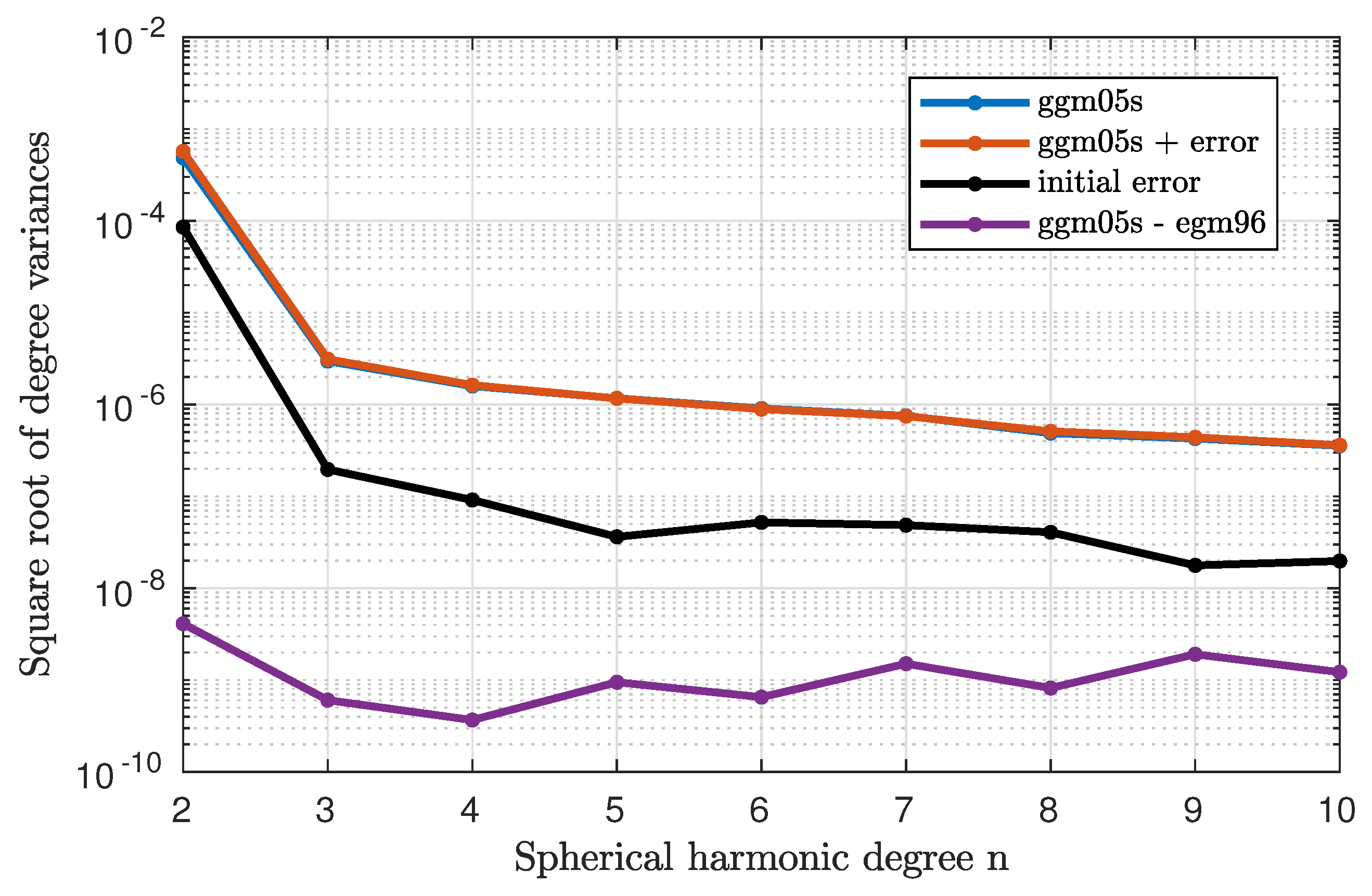
In Figure 1, the original (true) gravity field (GGM05S), which is used to produce the observations and the disturbed field, which is used as initial guess in the estimation process and the difference between both gravity fields are shown. All gravity fields are shown in the form of square root of degree variances. Additionally, for comparison, the difference between GGM05S and Earth Gravitational Model 1996 (EGM96) [18] is also plotted. This shows that the imposed initial gravity field error is quite big.

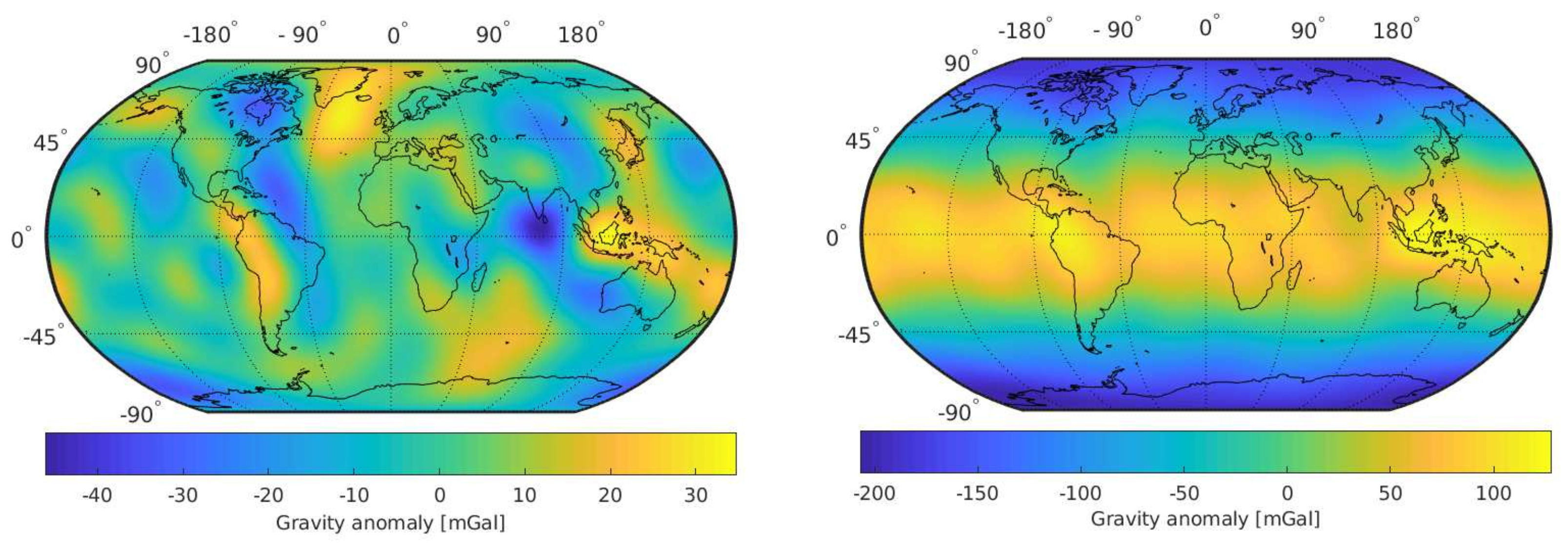
The true (GGM05S) and the initial gravity fields are shown spatially in terms of gravity anomalies in Figure 2. Both plots show the gravity fields up to degree and order 10. In these plots, the initial error is visible quite distinctly. The big error on the $C_{20}$ coefficient overlays nearly all other features of the gravity field.

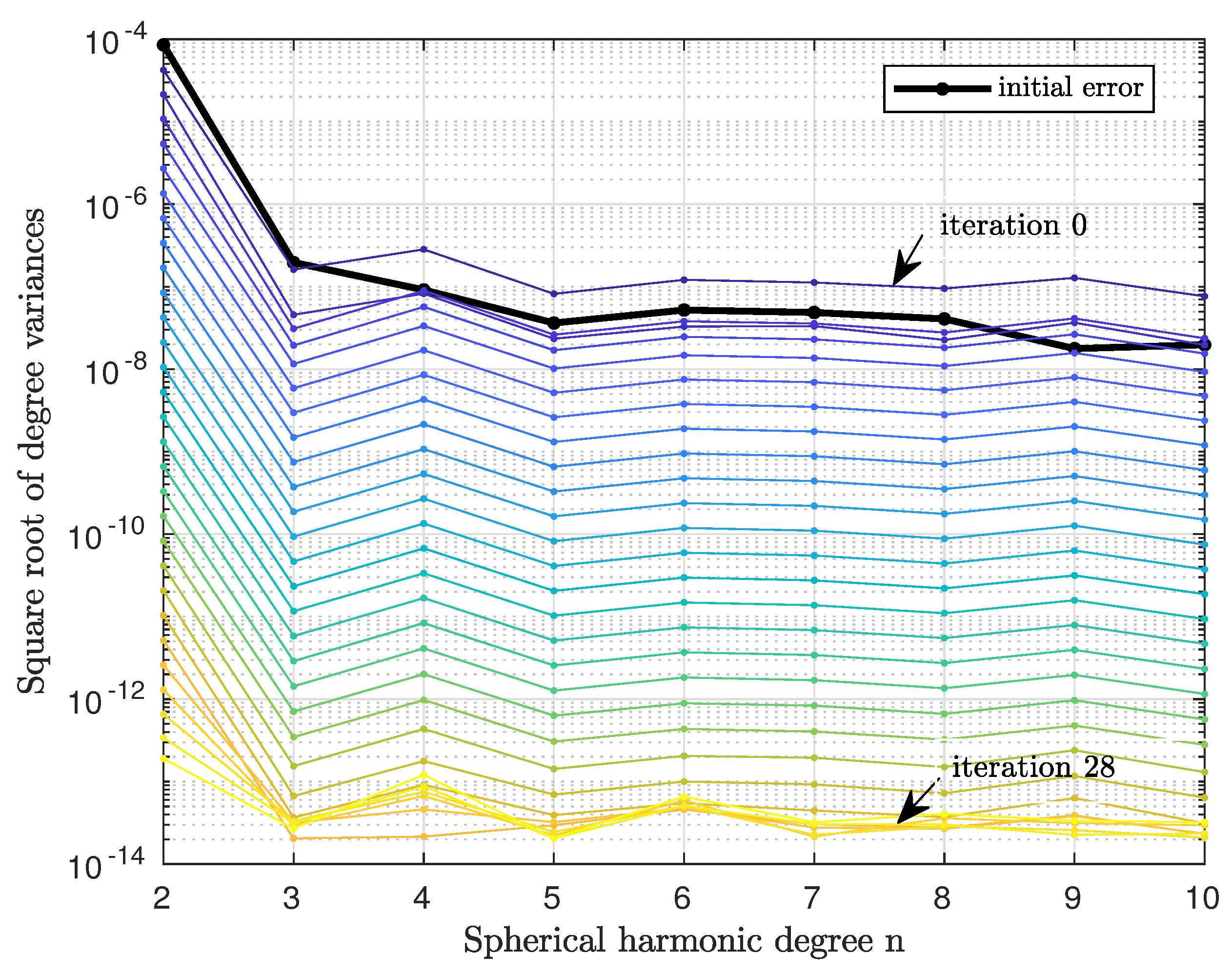
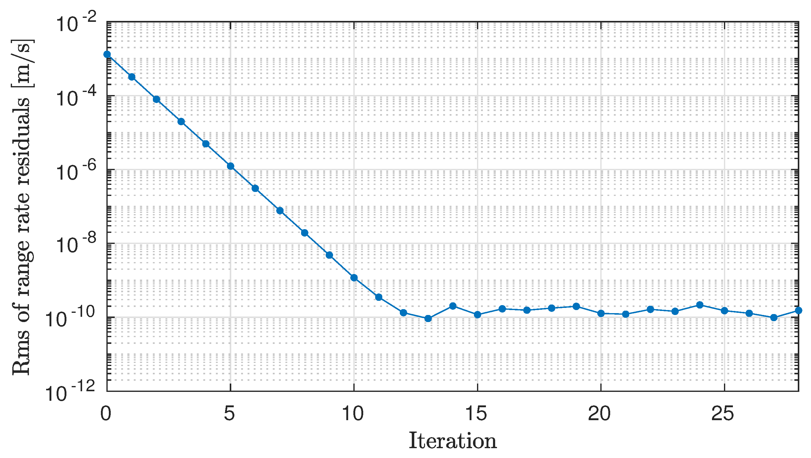
To recover the gravity field, we use four days of simulated data and a local arc length of one day. The perfect initial states for each arc are used. The difference between the estimated gravity field after each iteration with respect to the true field is shown in Figure 3 for 28 iterations. While the lower degrees (2 and 3) improve with the first iteration, the higher degrees are getting a bit worse and start improving after some iterations because there is a big difference between the initial and true gravity field for the lower degrees (2 and 3). After the fifth iteration, all degrees are improving subsequently with further iterations up to a square root of degree variances of about $2\times {10}^{-14}$. After this value is reached, further iterations are not improving the result anymore. Because the deviations of the spherical harmonic coefficients ($\widehat{\overrightarrow{c}}$) have reached the order of ${10}^{-15}$ to ${10}^{-16}$, which is the border of the double data type precision.

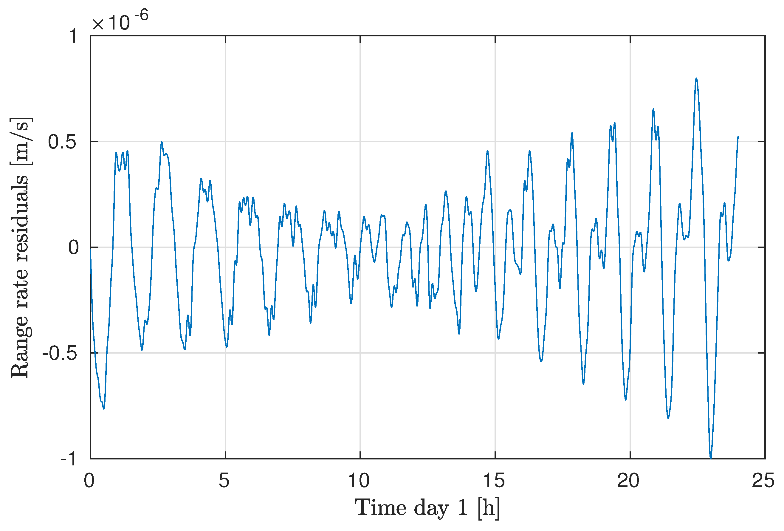
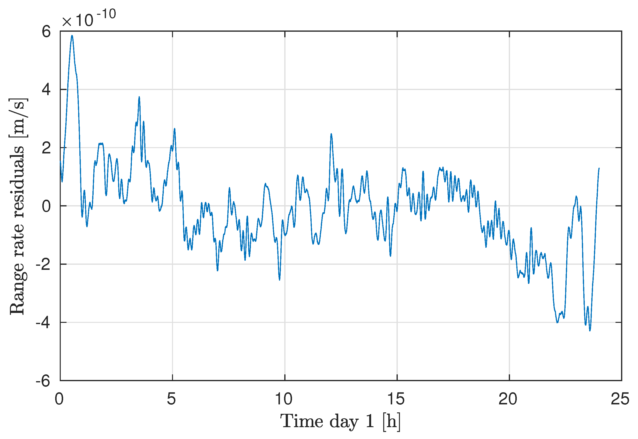
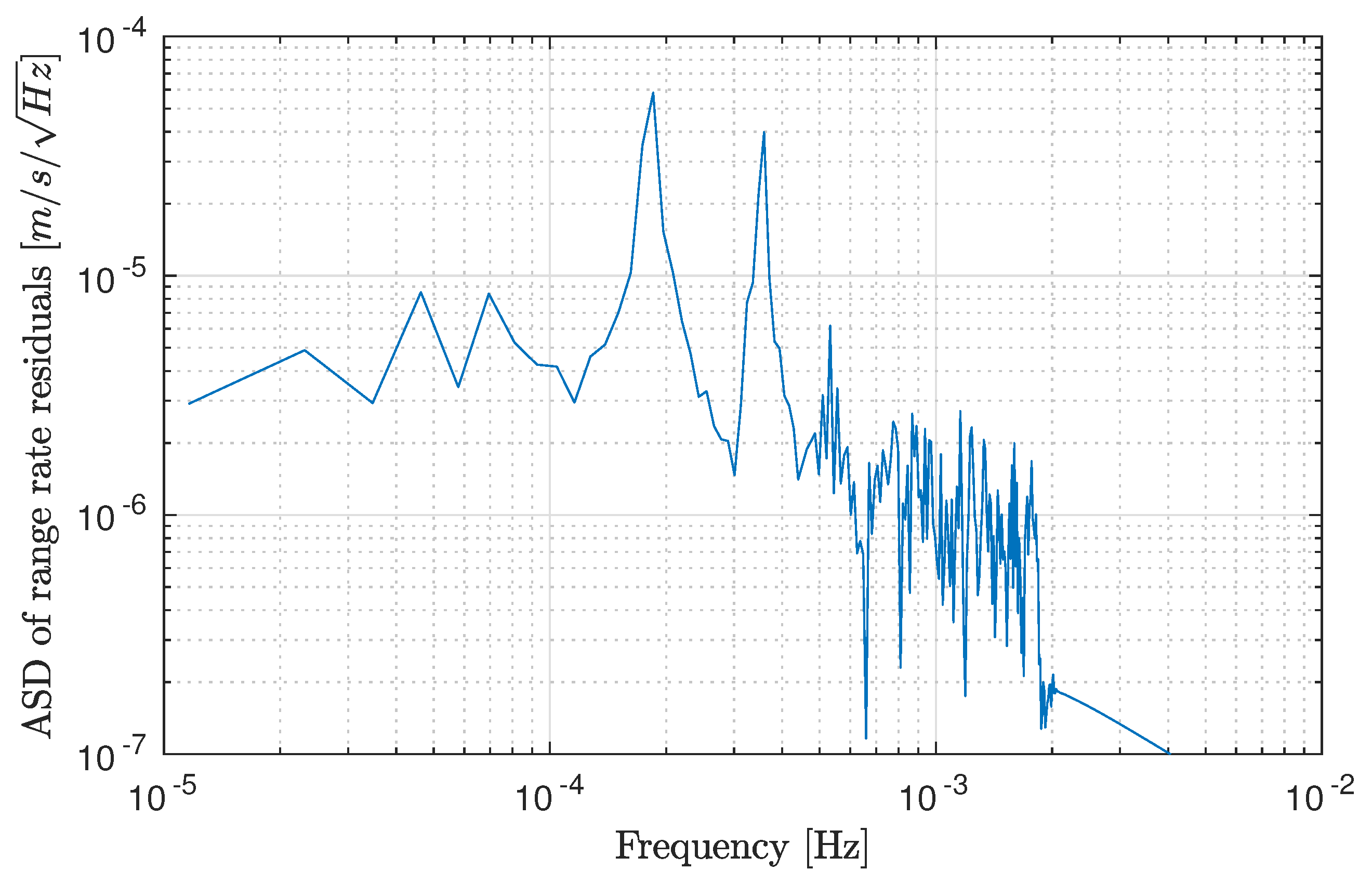
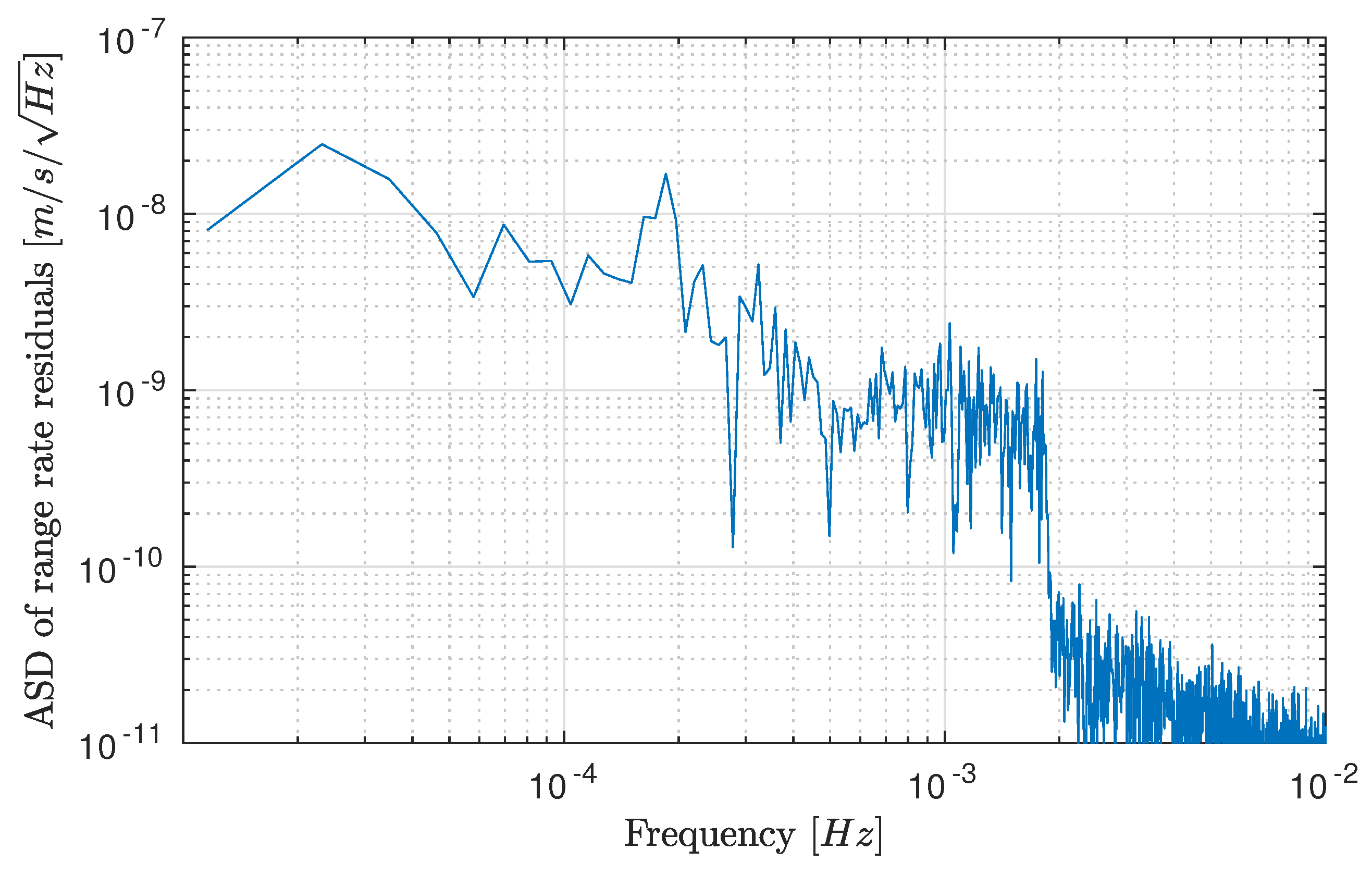
Until about Iteration 12, the resulting range rate residuals $\overrightarrow{ϵ}$ are decreasing. After Iteration 12, they stay at the same level of about some ${10}^{-10}$ m/s. Exemplarily, the range rate residuals for Day 1, for the sixth and last iteration (Iteration 28) are shown in Figure 4 and Figure 5. The evolution of the range rate residuals over all iterations is displayed in Figure 6, also for Day 1. The root mean square (rms) of the range rate residuals is computed and plotted over all iterations. This demonstrates that the residuals do not decrease further than ${10}^{-10}$ m/s. This is reasonable because this is about the numerical integration precision that is possible to archive for velocities (or relative velocities) with double precision data type. However, the gravity field coefficients can still be improved because, at this point, they are not limited by the integration error, but the linearization. The linearization error can be further reduced with subsequent iterations.

Additionally, in Figure 7 and Figure 8, the amplitude spectral density (ASD) of the range rate residuals are plotted. For the first iterations, two dominant peaks of one orbit and double orbit frequencies are visible. With further iterations, these peaks are decreasing more and more.

6. Conclusions

In this work, we have presented the first version of our new GRACE gravity field recovery code, written in MATLAB, using variational equations, which we call GRACETOOLS. The current version of our code provides an environment to evolve a gravity field recovery tool using GRACE satellites type observations. This first release of GRACETOOLS has been mainly focused on recovering a gravity field from simulated GRACE range rate observations. The on-going development of GRACETOOLS includes more sophisticated end to end simulations with all input force models and GRACE Follow-On instrument observations. We hope that, with the transparency provided by opening up the code, we can address open questions in GRACE data analysis faster and more efficiently.

References

- Tapley, B.D.; Bettadpur, S.; Watkins, M.; Reigber, C. The gravity recovery and climate experiment: Mission overview and early results. Geophys. Res. Lett. 2004, 31, L09607. [Google Scholar] [CrossRef]
- Rummel, R.; van Gelderen, M.; Koop, R.; Schrama, E.; Sansó, F.; Brovelli, M.; Miggliaccio, F.; Sacerdote, F. Spherical Harmonic Analysis of Satellite Gradiometry; Publications on Geodesy, New Series 39; Netherlands Geodetic Commission: Delft, The Netherlands, 1998. [Google Scholar]
- Naeimi, M.; Flury, J. Global Gravity Field Modeling from Satellite-to-Satellite Tracking Data. In Lecture Notes in Earth System Sciences; Springer: Berlin, Germany, 2017. [Google Scholar]
- Reigber, C. Gravity field recovery from satellite tracking data. In Theory of Satellite Geodesy and Gravity Field Determination; Springer: Berlin/Heidelberg, Germany, 1989; pp. 197–234. [Google Scholar]
- Jekeli, C. The determination of gravitational potential differences from satellite-to-satellite tracking. Celest. Mech. Dyn. Astron. 1999, 75, 85. [Google Scholar] [CrossRef]
- Han, S.-C.; Shum, C.K.; Jekeli, C. Precise estimation of in situ geopotential differences from GRACE low-low satellite-to-satellite tracking and accelerometer data. J. Geophys. Res. 2006, 111, B04411. [Google Scholar] [CrossRef]
- Beutler, G.; Jäggi, A.; Mervart, L.; Meyer, U. The celestial mechanics approach: Theoretical foundations. J. Geod. 2010, 84, 605–624. [Google Scholar] [CrossRef]
- Jäggi, A. Pseudo-Stochastic Orbit Modeling of Low Earth Satellites Using the Global Positioning System. Ph.D. Thesis, Astronomical Institute, University of Bern, Bern, Switzerland, 2006. [Google Scholar]
- Liu, X. Global Gravity Field Recovery From Satellite-to-Satellite Tracking Data With the Acceleration Approach. Ph.D. Thesis, Nederlandse Commissie voor Geodesie Netherlands Geodetic Commission, Delft, The Netherlands, 2008. [Google Scholar]
- Mayer-Gürr, T. Gravitationsfeldbestimmung aus der Analyse kurzer Bahnbögen am Beispiel der Satellitenmissionen CHAMP und GRACE. Ph.D. Thesis, Universitäts-und Landesbibliothek Bonn, Bonn, Germany, 2006. [Google Scholar]
- Keller, W.; Sharifi, M. Satellite gradiometry using a satellite pair. J. Geod. 2005, 78, 544. [Google Scholar] [CrossRef]
- Sakumura, C.; Bettadpur, S.; Bruinsma, S. Ensemble prediction and intercomparison analysis of GRACE time-variable gravity field models. Geophys. Res. Lett. 2014, 41, 1389–1397. [Google Scholar] [CrossRef] [Green Version]
- Gunter, B.C. Parallel Least Squares Analysis of Simulated GRACE Data. Master’s Thesis, The University of Texas at Austin, Austin, TX, USA, 2000. [Google Scholar]
- McCullough, C.M. Gravity Field Estimation for Next Generation Satellite Missions. Ph.D. Thesis, The University of Texas at Austin, Austin, TX, USA, 2017. [Google Scholar]
- Tapley, B.D.; Schutz, B.E.; Born, G.H. Statistical Orbit Determination; Elsevier Academic Press: Amsterdam, The Netherlands, 2004. [Google Scholar]
- Mayer-Gürr, T.; Behzadpour, S.; Ellmer, M.; Kvas, A.; Klinger, B.; Zehentner, N. ITSG-Grace2016—Monthly and Daily Gravity Field Solutions from GRACE. GFZ Data Services. 2016. Available online: http://doi.org/10.5880/icgem.2016.007 (accessed on 11 September 2018).
- Ries, J.; Bettadpur, S.; Eanes, R.; Kang, Z.; Ko, U.; McCullough, C.; Nagel, P.; Pie, N.; Poole, S.; Richter, T.; et al. Development and Evaluation of the Global Gravity Model GGM05-CSR-16-02; Technical Report for Center for Space Research; The University of Texas: Austin, TX, USA, 2016. [Google Scholar]
- Lemoine, F.G.; Kenyon, S.C.; Factor, J.K.; Trimmer, R.G.; Pavlis, N.K.; Chinn, D.S.; Cox, C.M.; Klosko, S.M.; Luthcke, S.B.; Torrence, M.H.; et al. The Development of the Joint NASA GSFC and the National Imagery and Mapping Agency (NIMA) Geopotential Model EGM96; NASA: Washington, DC, USA, 1998.
- Chung, L.R. Orbit Determination Methods for Deep Space Drag-Free Controlled Laser Interferometry Missions. Master’s Thesis, University of Maryland, College Park, ML, USA, 2006. [Google Scholar]
Figure 1.
Square root of degree variances from true gravity field (GGM05S), with which observations were simulated, initial gravity field for the estimation process, and the difference between both fields. As comparison the difference between GGM05S and EGM96 is also shown.
Figure 2.
True (GGM05S) gravity field (left) and initial gravity field (right) in terms of gravity anomalies up to degree and order 10.
Figure 3.
Square root of degree variances of difference between true gravity field and estimated fields after each iteration.
Figure 4.
Time series of range rate residuals for Day 1 after the sixth iteration.
Figure 5.
Time series of range rate residuals for Day 1 after the last (28th) iteration.
Figure 6.
Root mean square (rms) of range rate residuals for Day 1, for each iteration
Figure 7.
Amplitude spectral density of range rate residuals for Day 1 after the sixth iteration.
Figure 8.
Amplitude spectral density of range rate residuals for Day 1 after the last (28th) iteration.