Identifying Karst Aquifer Recharge Areas using Environmental Isotopes: A Case Study in Central Italy

Abstract

Water resources management is one of the most important challenges worldwide because water represents a vital resource for sustaining life and the environment. With the aim of sustainable groundwater management, the identification of aquifer recharge areas is a useful tool for water resources protection. In a well-developed karst aquifer, environmental isotopes provide support for identifying aquifer recharge areas, residence time and interconnections between aquifer systems. This study deals with the use of environmental isotopes to identify the main recharge area of a karst aquifer in the Upper Valley of Aniene River (Central Italy). The analysis of ¹⁸O/¹⁶O and ²H/H values and their spatial distribution make it possible to trace back groundwater recharge areas based on average isotope elevations. The Inverse Hydrogeological Balance Method was used to validate spring recharge elevations obtained by the use of stable isotopes. Areas impacted by direct and rapid rainfall recharge into the study area were delineated, showing groundwater flowpaths from the boundaries to the core of the aquifer. The results of this study demonstrate the contribution that spatial and temporal isotope changes can provide to the identification of groundwater flowpaths in a karst basin, taking into account the hydrogeological setting.

1. Introduction

Karst aquifer protection is the most important environmental factor for water sustainable management worldwide, as groundwater coming from karst aquifers is a key source of freshwater for human supply.

Due to the impacts of climate change and the increase of anthropogenic activities, groundwater exploitation in karst aquifers requires special strategies to prevent their quality and quantity depletion and to support water resources management [1,2]. Karst aquifers are characterized by spatial and temporal complexity of karst flowpaths, caused by high heterogeneity of the rock matrix, large voids, and high flow velocities [3]. Water flow velocities into a well-developed karst system are extremely fast and contaminants can quickly reach the saturated zone, making these hydrogeological systems particularly vulnerable to contamination. This system may receive localized inputs from sinking surface streams and as storm runoff through sinkholes, dolines and karst features in general. For this reason, in a karst setting, the identification of these fast recharge areas is an important tool in order to protect groundwater resources [4].

In hydrogeological studies of karst aquifers, the application of tracers can be considered as an advanced method that allows for an integrative investigation, with the aim of effective management of water resources [5]. Environmental and artificial tracers are used more and more often in hydrogeology to investigate groundwater flow paths. In particular, they are applied to trace water flows inside the hydrological cycle from infiltration, influenced by chemical and isotopic precipitations, to discharge due to water–rock interactions and geochemical processes [6,7,8,9,10,11,12]. At present, there are more than 1000 known isotopes of about 92 chemical elements. Most of these isotopes are either stable or unstable [5]. Naturally, occurring stable isotopes of water have been used extensively in hydrological investigations over the past few decades [13,14,15]. In particular, the traditional stable isotope ratios of hydrogen and oxygen (²H/H and ¹⁸O/¹⁶O) are recognizable tracers that are related to the water cycle and have been widely used in hydrology and water resources for decades [16]. These isotopes are often applied in hydrogeological investigations to study precipitation, groundwater recharge, groundwater-surface water interactions, delineation of flow systems and quantification of mass-balance relationships [13]. The spatial and temporal variations of stable hydrogen and oxygen isotopes in precipitations are affected by moisture sources, elevation, temperature, rainfall amount, latitude, and distance from oceans [17,18]. The seasonal cycles of stable isotope tracers in water can be used to characterize the mean transit time of catchments, which is the average travel time for water parcels to enter as precipitation and leave as streamflow within catchments, but recent studies have shown that most of these calculations have errors of several hundred percent because of aggregation bias [18,19]. Spatial and temporal variations in stable isotopes of rainfalls are related to the isotopic fractionation process, accompanying evaporation from the ocean and condensation during the atmospheric transport of water vapor [20,21]. Other factors that influence the water isotopic content, several of which are closely related to temperature, include the following: atmospheric moisture, rainfall amount, latitude, elevation, continental and seasonal effects [17,20,21,22]. In hydrology, fractionation of δ¹⁸O and δ²H is driven by kinetic processes during evaporation and condensation [20]. During the evaporation process of oceanic water, a sequence of isotope fractionations involves variations in the precipitation isotopic composition, which are reflected in continental meteoric water. Since this fractionation process is based on the equilibrium of the isotope ratios between the vapor and liquid states of water, a specific relationship represents the distributions of isotope values of oxygen and hydrogen in rainfall [5,13]. Light variations of isotopic concentrations are usually measured by mass spectrometry. In general, isotopic abundance ratios are expressed as parts per million of their deviations, as given by (Vienna Standard Mean Ocean Water, VSMOW) Equation (1):

$$\mathsf{\delta }=\frac{\left({\mathrm{R}}_{\mathrm{sample}}-{\mathrm{R}}_{\mathrm{SMOW}}\right)}{{\mathrm{R}}_{\mathrm{SMOW}}}\times {10}^3$$

(1)

where R = ²H/H for hydrogen and ¹⁸O/¹⁶O for oxygen, the ratio of the heavy to light isotope [23], due to the significant geographical and temporal variations in the isotopic composition of precipitation [20,24], and R_SMOW is the isotopic ratio of the standard (Standard Mean Ocean Water).

The application of stable isotope ratios of hydrogen and oxygen of groundwater can provide information about springs recharge elevation, only in terms of relative values. Only the comparison between the oxygen and hydrogen isotopic compositions of precipitation and groundwater allows the evaluation of recharge elevation values and consequently the identification of aquifer recharge areas. Thus, in this paper, a combined approach has been applied, based on the application of the Inverse Hydrogeological Balance Method [25] and the natural occurring of stable isotope ratios of oxygen and hydrogen, to identify the boundaries of the main infiltration areas of a karst aquifer in Central Italy.

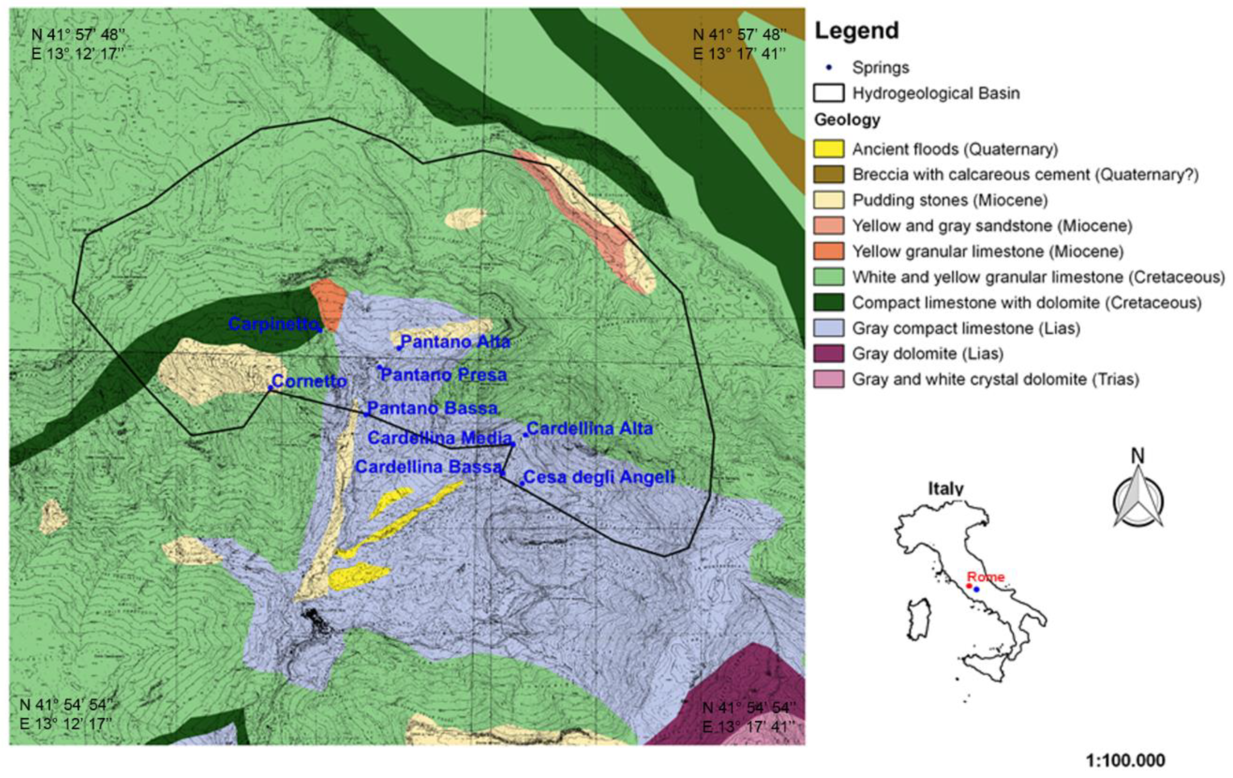
2. Geological and Hydrogeological Setting

The Simbruini Mountains karst aquifer is located in southern Latium Region (Central Italy), 60 km southeast of Rome and 65 km inland from the Tyrrhenian Sea, in the Upper Valley of the Aniene River, within the Simbruini Mountains Regional Park. Karst springs are numerous along the first part of the Aniene and are the most important water resources in the southeast part of the Latium Region, supplying drinking water to the city of Rome. In this study, nine springs feeding the Simbrivio water supply system (

Table 1. Sampling location of the study area.

Sample Codes	Spring	Lng (m)	Lat (m)	Elevation (m a.s.l.)
GW1	Cardellina Alta	4,645,069	355,391	1057
GW2	Cardellina Media	4,644,978	355,274	989
GW3	Cardellina Bassa	4,644,703	355,176	939
GW4	Cesa degli Angeli	4,644,606	355,359	940
GW5	Cornetto	4,645,520	352,959	945
GW6	Carpinetto	4,646,065	353,431	960
GW7	Pantano Alta	4,645,896	354,187	952
GW8	Pantano Bassa	4,645,547	354,012	901
GW9	Pantano Presa	4,645,714	353,999	830

) in the Simbruini Mountains karst aquifer, based on data availability, were examined. The hydrogeological basin of these karst springs, of about 15 km², is shown in Figure 1.

The lithological sequence outcropping in the Upper Valley of the Aniene River includes the North-West part of the Lower-Middle Miocene Latium-Abruzzi Carbonate Platform [26,27,28,29].

The stratigraphic succession of dolomite, dolomitic limestone and limestone is distributed homogeneously from North to South and from East to West in the study area [30]. The Triassic series outcrops among Filettino, Aniene River Springs and Faito Plateau. Dolomite is the dominant lithofacies, characterized by white and grey crystalline dolomite, with some breccia levels. Over this geological formation, limestones and dolomites, of Upper Cretaceous age are present, and their immersion is concordant with the Triassic dolomite [29,30]. In fact, the Aniene basin is composed almost entirely of bare Mesozoic, highly fractured, karstified carbonate rocks of the central Apennine range [31]. This area is mostly made of highly permeable Cretaceous carbonate rocks, deeply fractured and mostly soluble. The base of the stratigraphic series is made of Upper Cretaceous carbonates, represented by the alternation of granular limestone and dolomites layers (Figure 1).

Above these ones lie Quaternary fluvial and alluvial deposits, conglomerate, Miocene clay, and shale [31,32]. The carbonate deposits that form the structure of the hills are typically monoclinal with immersion of the strata to the N-NE and inclinations of approximately 40–45° [32,33]. Due to chemical weathering, a distinctive surface and underground karst formations are developed in this area at small and large scales. The surface karst activity has led to the formation of a typical karst landscape with rutted fields, sinkholes and red soils, while the underground activity has given rise to cavities, ponor and cave systems [29,30]. The karst surface is very permeable and enables the rapid infiltration of rainfall into the underground system, where the carbonate dissolution makes cavities [29,30]. Dissolution conduits strongly influence groundwater flow and evolve into complex networks, often crossing several kilometers throughout the limestone matrix [34,35,36]. The basin is characterized by both point and diffuse recharge. Recharge to the groundwater system is primarily dispersed over the basin from precipitation and secondarily concentrated at sinkholes and losing streams. The spring discharge responds immediately to increases in precipitation, especially after heavy rainfalls (from October to April).

3. Materials and Methods

Groundwater samples were collected during the wet season (June 1997) and the dry season (October 2002) to investigate seasonal variations. Eighteen water samples, coming from nine karst springs across the study area, were analyzed by the Isotope Geochemistry Laboratory of the University of Parma (Italy) using the IRMS (Isotope-ratio mass spectrometry) continuous flow-equilibration method with CO₂ for δ¹⁸O and H² for δ²H.

The results (

Table 2. Isotope composition of spring water samples collected in October 2002 and in June 1997.

Sample Codes	June 1997			October 2002
	δ18O (‰VSMOW)	δ2H (‰VSMOW)	dexcess (‰)	δ18O (‰VSMOW)	δ2H (‰VSMOW)	dexcess (‰)
GW1	−8.4	−57	10.6	−8.7	−50	19.2
GW2	−9.0	−63	9.1	−8.7	−53	17.2
GW3	−8.6	−59	9.4	−8.8	−52	18.7
GW4	−9.1	−62	10.8	−9.1	−52	20.7
GW5	−8.2	−56	9.5	−8.4	−48	19.5
GW6	−9.1	−62	10.9	−8.7	−50	20.0
GW7	−8.6	−60	9.4	−8.8	−52	19.1
GW8	−8.6	−60	8.9	−8.9	−50	19.7
GW9	−8.7	−60	9.2	−8.8	−51	20.9

) are expressed as per million deviations from the internationally accepted standard VSMOW (Vienna Standard Mean Ocean Water) according to Equation (1) [14]. The analytical error is ±0.2‰ for δ¹⁸O and ±1‰ for δ²H.

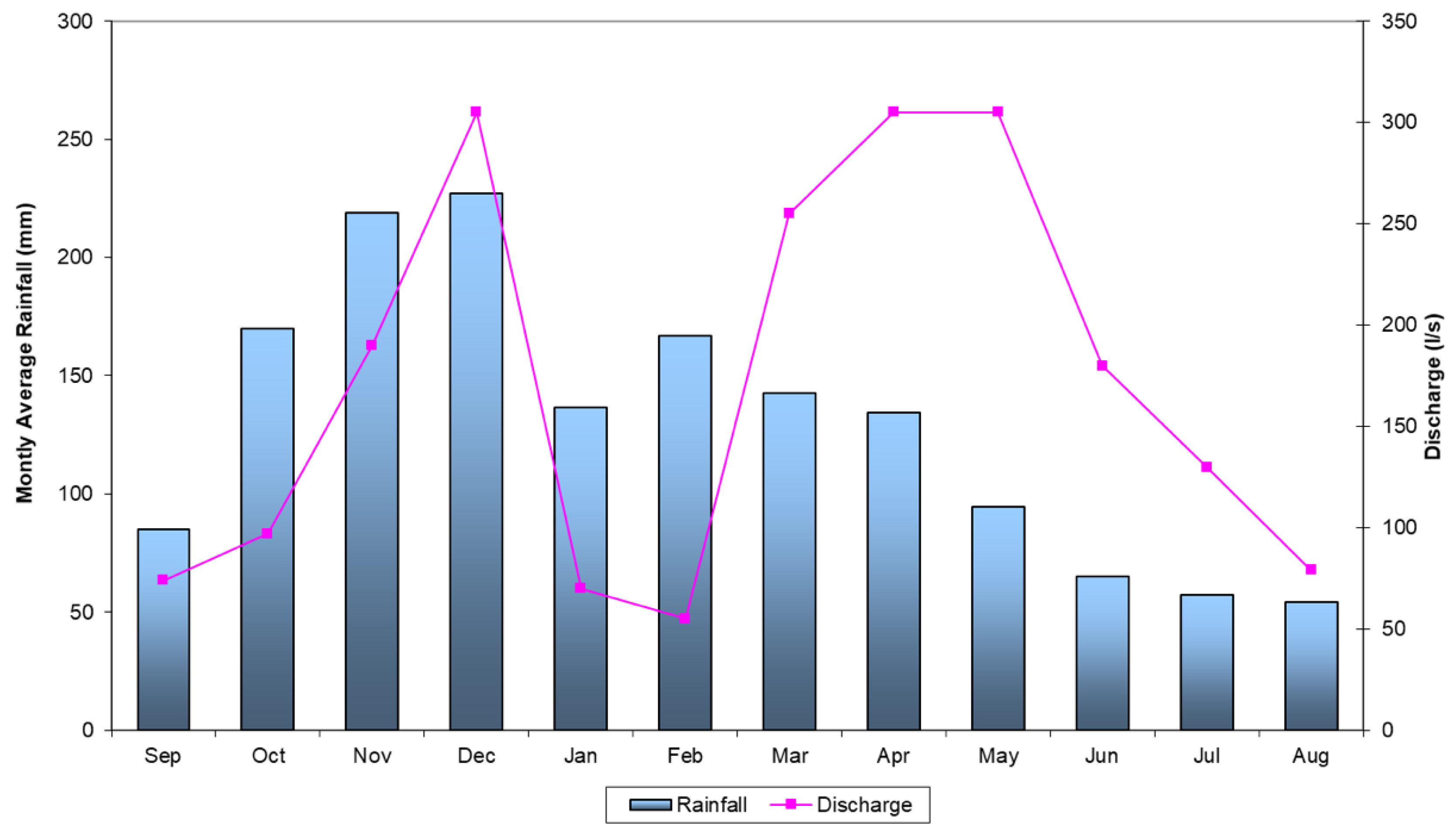
4. Results and Discussions

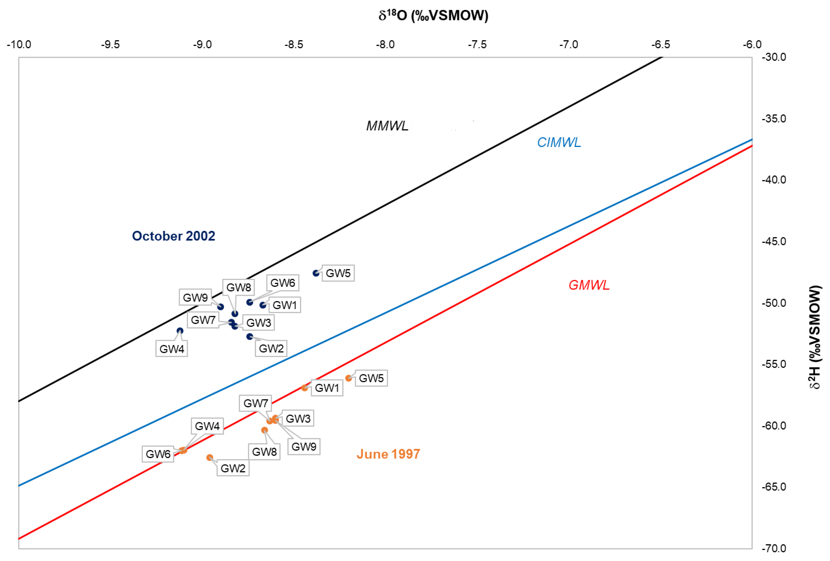
4.1. Oxygen and Hydrogen Isotope Composition

Groundwater samples from June 1997 have δ¹⁸O contents within a range from a minimum of −8.2‰ VSMOW (GW5) and a maximum of −9.11‰ VSMOW (GW6), and with an average of −8.70‰ VSMOW. For ²H, the average value is −59.82‰ VSMOW with a maximum of −62.55‰ VSMOW (GW2) and a minimum of −56.10‰ VSMOW (GW5) (Table 2). In the October 2002 samples, the δ¹⁸O values vary from −9.12‰ VSMOW (GW4) to −8.38‰ VSMOW (GW5) with an average of −8.78‰ VSMOW, and δ²H values range from −52.71‰ VSMOW (GW2) to −47.55‰. VSMOW (GW5) (Table 2). These changes, as mentioned above, are controlled by hydrological parameters, including temperature, precipitation, altitude, latitude and seasonal effects [16,17,20,21,22]. A seasonal oscillation of stable isotope ratios is often observed as a result of temperature [5].

To study the overall stable isotopic characteristics of the spring samples, the isotope concentration values for June 1997 and October 2002 were plotted, together with the Global Meteoric Water Line (GMWL) [17,23], the Mediterranean Meteoric Water Line (MMWL) [35] and the Central Italy Meteoric Water Line (CIMWL) [37] (Figure 2).

Groundwater samples of June 1997 are located along the Global Meteoric Water Line (GMWL) of Gourcy (2005) (δ²H‰ = 8.14 (±0.02) * δ¹⁸O‰ + 10.9(±0.2); R = 0.98), indicating that rainfall is the primary source of groundwater. The plot of δ²H values versus δ¹⁸O for spring samples of October 2002 more close to the (MMWL) (δ²H‰ = 8δ¹⁸O‰ + 22) [38], showing more δ¹⁸O enrichment in comparison with δ²H and suggesting input from local rainfall coming from the Mediterranean Sea. The regression lines of the samples have different slopes, which are mainly related to local evaporation effect [24]. This difference applies to samples collected in two different seasons, June and October. In the wet season (2002 samples), the hydrogen and oxygen isotopes showed a depleted composition compared those of the dry season (1997 samples). The amplitude of these isotopic variations is directly related to the changing of the seasonal temperature. The distribution of hydrogen and oxygen isotopic composition in groundwater samples of Figure 2 provides an initial understanding of the origin of groundwater in the study area. The examination of the relationship ²H/¹⁸O shows that the measured values of June 1997 and October 2002 samples align with Equations (2) and (3), respectively.

$$\mathsf{\delta }{}^2\mathrm{H}‰=6.95\mathsf{\delta }{}^{18}\mathrm{O}‰+0.64(\mathrm{R}=0.898)$$

(2)

$$\mathsf{\delta }{}^2\mathrm{H}‰=5.93\mathsf{\delta }{}^{18}\mathrm{O}‰+1.30(\mathrm{R}=0.564)$$

(3)

Several processes are responsible for the deviation of water samples from the local meteoric water line. Evaporation from surface bodies is a nonequlibrium process that enriches residual water bodies such that the δ²H/δ¹⁸O slope is less than 8, and is often between 3 and 6 [13]. The slope is a function of humidity, salt concentration, and other factors [21]. In both, the slope is as low (<8) as that determined by the GMWL, with the equation defined by Craig (1961)—δ²H‰ = 8δ¹⁸O‰ + 10—indicating a meteoric groundwater origin. Therefore, it appears that this slope shows that waters are affected by a slight phenomenon of evaporation before infiltration [16,23]. The 2002 evaporation line (3) has a slope of 5.93, which is less than the GMWL slope of 8.17 [17], less than the CILML gradient of 7.047 [37] and also less than the 1997 evaporation line (2) gradient of 6.95.

The ²H excess value is a function of several factors, such as the temperature, humidity, and the isotopic characteristics of the environment water vapor and the evaporating water. The value of d may differ significantly from area to area and over geologic time. The d-excess factor has been shown to be a diagnostic tool for measuring the contribution of evaporated moisture to the downwind atmosphere. High d-excess values generally indicate that more evaporated moisture has been added to the atmosphere [40,41], and low values are associated with samples fractionated by evaporation. Previous studies have shown that the western part of the Mediterranean basin has a d-excess of +14‰, whereas the eastern part shows an excess of +22‰ (Eastern Mediterranean) [42], and this variation reflects a mixture between the Mediterranean and the Atlantic air masses [43,44]. These high values are probably related to strong isotopic kinetics occurring in the summer during the evaporation process above the Mediterranean Sea, and due to the low relative humidity of the atmosphere. Groundwater samples in the study area present d-excess values in the range of +8.93 to 10.88‰ in June 1997 and of +17.21 to +20.90‰ in October 2002, with an average of 9.78 to 19.46‰, respectively (Table 2). These values include the range from 10, for global precipitation, to 22, for the eastern Mediterranean area, indicating the significance of the Mediterranean as a moisture source for Italy [15,44]. Most of the spring samples with high deuterium excess values (October 2002) suggest that the precipitation in the groundwater comes from the Mediterranean sector. On the contrary, groundwater sampled in June 1997 shows low d-excess values (ranging from 8.93 to 10.88‰). Based on that isotopic diagram of Figure 3, the first meaningful assessments were made regarding which springs were fed from the highest elevation areas and which ones from the lowest ones. First, GW4 water samples are the poorest in heavy isotopes, suggesting that Cesa degli Angeli spring has a higher infiltration elevation than all the other ones (Figure 2). The plot of δ²H values versus δ¹⁸O for water samples from the Pantano group (GW7, GW8 and GW9) shows a similar isotopic composition, suggesting the same recharge area. The same approach can be applied to GW1, GW2 and GW3 springs, whose isotopic values are depicted as a group. Lastly, water samples coming from Carpinetto spring (GW6) show different isotopic behavior referring to the sampling season. As a matter of fact, samples collected in June seem to be depleted in heavy isotopes of hydrogen, while this fact is not clear in ones taken in October. These different behaviors could be related to the different flow paths of groundwater coming out from Carpinetto spring. The GW6 sample collected in June was infiltrated in winter. During that season, the air masses come from the Atlantic reservoir. On the other hand, the sample collected in October is rich in heavy isotopes, because it is groundwater, infiltrated in summer, with a short residence time. GW5 water samples show the heaviest content in heavy isotopes in both seasons, highlighting that the Cornetto spring is indeed fed at a lower elevation than all the other ones. However, it is impossible to define the groundwater infiltration elevations based on the sample positions on the isotopic diagram without having precipitation markers as a reference.

To better identify the above-mentioned recharge periods, average monthly precipitation for the twenty-year period 1951–1999 was calculated for the Vallepietra pluviometric station. The evolution of the rainfalls and the outflow diagram of the Carpinetto spring (GW6) is reported in Figure 3. The other springs analyzed in this study show similar behavior.

Based on fifty-year rainfall data, Figure 3 shows that the maximum and the minimum precipitation average values occur in November/December and in August, respectively. The evolution of the outflow diagram of the Carpinetto spring (GW6), as compared to the monthly average rainfall, shows a delay between the maximum precipitations, reached in November/December, and the maximum flow coming from GW6 in May. In general, not only for GW6, as represented in Figure 3, with regard to the hydrological regimes of the springs under study, there is an average delay of about six months between the meteoric inflow and the discharge of the springs.

Spring water samples collected in June refer to the main recharge period of the year (November and December), when rainfalls drop from clouds coming from the Atlantic, and are therefore considerably less rich in heavy isotopes. On the contrary, samples collected in October refer to waters infiltrated during summer months, when rainfall comes from clouds formed in the Mediterranean basin. These considerations have been useful in supposing, with acceptable reliability, that the aquifer residence time is about six months.

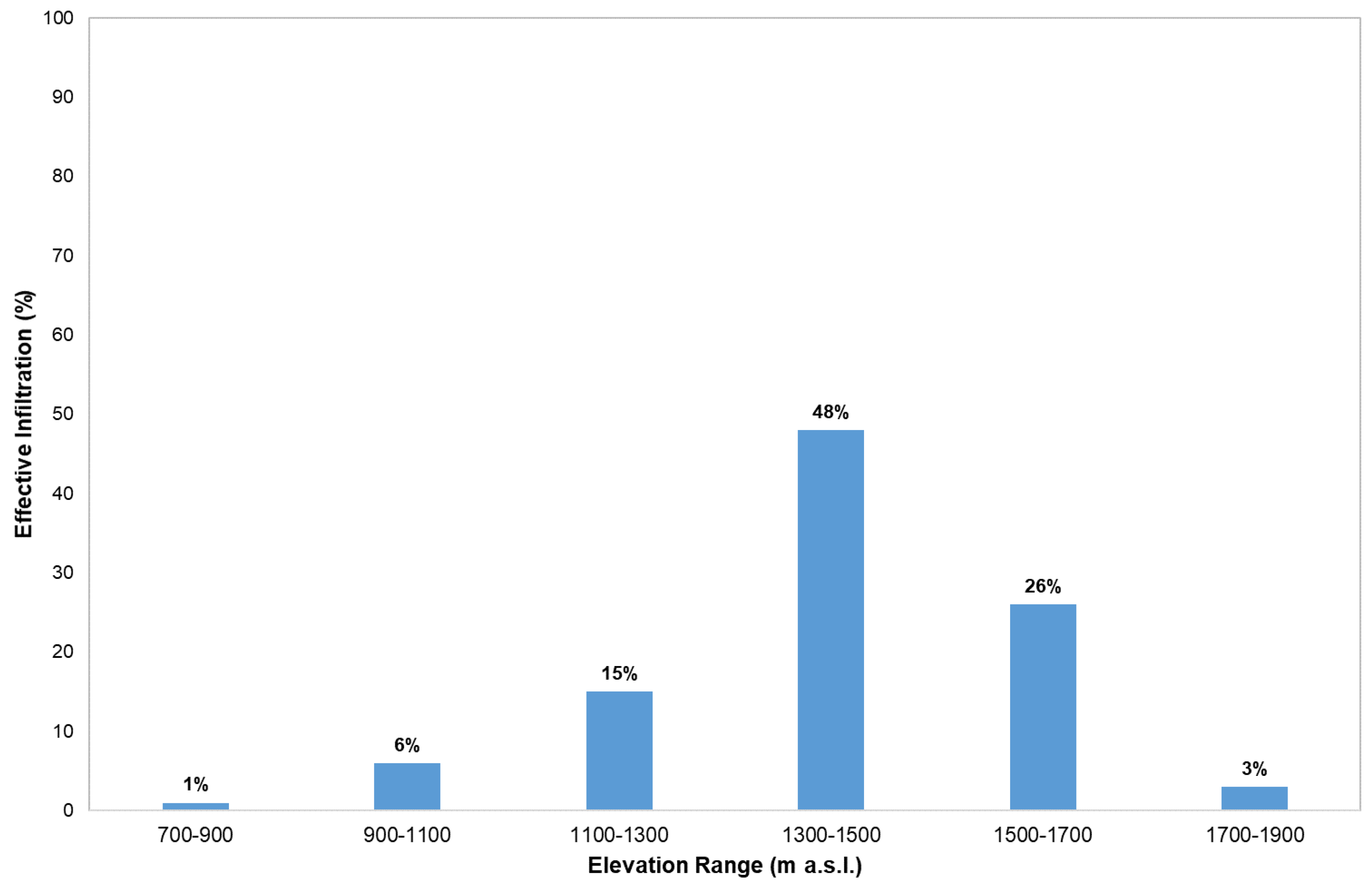
4.2. Spring Recharge Area Identification Using Isotope Analysis

The isotopic composition of groundwater in relation to elevation is an indicator for locating the groundwater recharge area [44]. In a given groundwater basin, groundwater sources may be fingerprinted using isotopes, like ²H and ¹⁸O, which depend on infiltration altitude of rainfalls. Higher altitude will have precipitation that is depleted in ²H and ¹⁸O. If the recharge source end members at different altitudes can be identified, it is possible to partition the amount of recharge to groundwater sampled from springs or in lowland areas accordingly [13]. As a matter of fact, fissured-karstic aquifers receive the recharge from the surrounding higher elevated areas. The high altitude contributes to more depletion in heavy isotopes in rainwater, and the joints and fractures of these aquifers supply good paths for transporting this infiltrated rainwater to the lower area. The distribution of the isotopic composition shows that, in mountain areas, heavy isotopes are more depleted than in the plain area [13]. At the highest elevations, where the average temperatures are lower, meteoric precipitation is characterized by depletion in heavy isotopes. For δ¹⁸O the depletion varies from −0.15 to −0.5‰ for each 100 m increase in elevation, with a corresponding decrease in δ²H oscillating between −1 and −4‰. The altitude effect is used in hydrogeological studies because it allows one to determine which recharge zones are located at higher or lower altitudes. As a result, due to the fact that isotopic tracers are conservative, the spring water that is supplied at higher elevations will be low in heavy isotopes, whereas an enrichment in heavy isotopes will be found in water that, once infiltrated into the aquifer, supplies the springs located at lower altitude. Many studies on this topic have emphasized that the value assumed by the gradient of isotopic content varies according to meteoclimatic characteristics [36]. The altitude effect is linked to the relation between rainfall isotope composition and elevation in meters. In this study, the average values of vertical isotopic gradient measured in Italy of about −0.15‰/100 m elevation for δ¹⁸O [37] and −1.2‰/100 m elevation for δ²H have been used. Vertical isotopic gradient evaluation, however, requires information about precipitation hydrogen and oxygen isotopic composition and their sampling altitudes. In this study, as the isotopic content of rainfall at specific elevations were not available, with the aim of calculating the mean recharge elevation of spring water samples, we applied two different methods to verify the reliability of the results obtained.

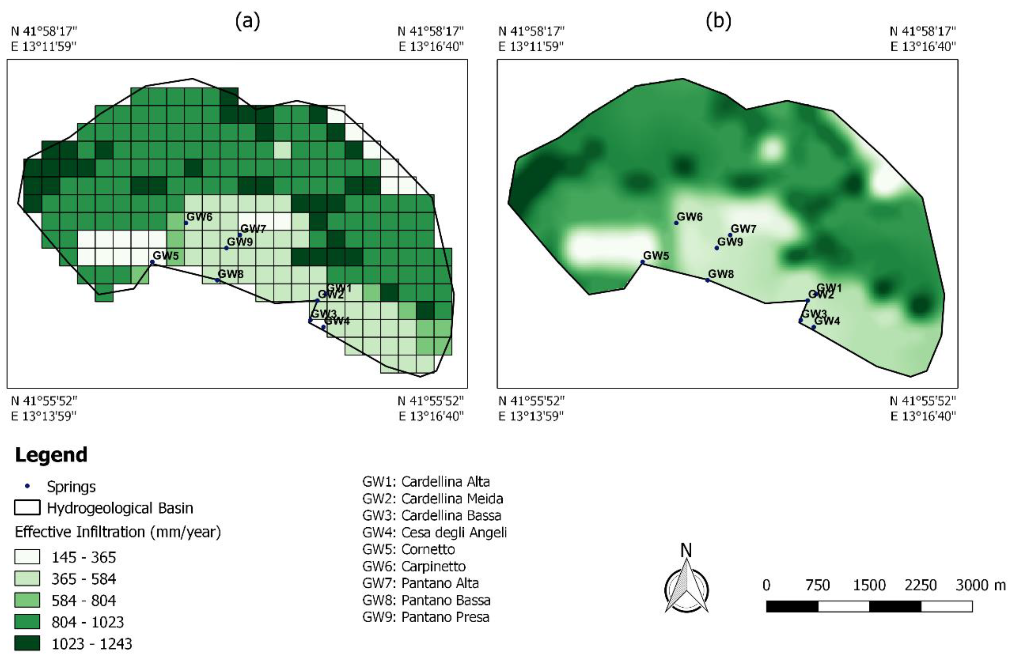
4.2.1. Center of Mass Method

The center of mass method is a concept of weighted average, used in solids mechanics. The center of mass is the point in an object or system of objects at which the whole mass may be considered as concentrated. The distribution of mass is balanced around the center of mass and the average of the weighted position coordinates of the distributed mass defines its coordinates.

In this study, the center of mass was considered to be a statistical and virtual point of the basin, where the whole infiltration of rainfall occurs. The Inverse Hydrogeological Balance Water Method [1] was used to evaluate the distribution of the average annual active recharge (i.e., the effective infiltration) within a GIS environment, discretizing the basin into Finite Squared Elements (FSE). Using this method, it can be possible to identify the center of mass of the basin, which defines to the hydrogeological characteristics of the basin. To apply the vertical isotopic gradients of oxygen and hydrogen, previously described, the procedure described below was chosen.

Water stable isotopes are conservative tracers of groundwater, related to rainfall’s isotopic composition before infiltration. With the aim of identifying the recharge areas of karst springs under study [20], the GW1 spring was chosen, which has the highest outcropping elevation in the hydrogeological basin (1057 m a.s.l.), and is reasonably closer than the others, in its groundwater isotopic content, to the rainfall value [13]. Thus, for GW1 spring, based on Equation (4), the average infiltration elevation was calculated, weighted according to the effective infiltration values obtained by the application of the Inverse Hydrogeological Balance Water Method (Figure 4):

$${\mathrm{z}}_{\mathrm{average}}=\frac{{{\displaystyle \sum }}_{\mathrm{i}=1}^{\mathrm{n}}{\mathrm{z}}_{\mathrm{i}}·{\mathrm{I}}_{\mathrm{i}}}{{\mathrm{I}}_{\mathrm{tot}}},$$

(4)

where z_i is the average elevation of the i^th FSE, I_i is the effective infiltration for the i^th FSE, n is the number of FSE into which the hydrogeological basin was previously discretized, and I_tot is effective infiltration calculated for the whole basin. The mean recharge elevation of any spring was calculated by the application of the vertical isotopic gradient, for ¹⁸O as for ²H, using the 2002 isotope values of δ¹⁸O (–8.67) and δ²H (–50.14) from the GW1 (Cardellina Alta) sample, which was the closest to the recharge area in the basin (

Table 3. Center of Mass Method—Average elevation of Cardellina Alta Spring (GW1).

Sample Codes	Spring	Average Elevation (m a.s.l.)	δ18O (‰VSMOW)	δ2H (‰VSMOW)
GW1	Cardellina Alta	1400	−8.67	−50.14

), as the end member.

Identified recharge elevations for each spring sample are presented in

Table 4. Recharge elevation obtained by the application of the Center of Mass Method.

Sample Codes	Recharge Elevation (m a.s.l.) δ18O (‰VSMOW)	Recharge Elevation (m a.s.l.) δ2H (‰VSMOW)	Average Recharge Elevation (m a.s.l.)
GW1	1400	1400	1400
GW2	1423	1503	1463
GW3	1448	1469	1459
GW4	1545	1484	1515
GW5	1306	1296	1301
GW6	1423	1391	1407
GW7	1455	1457	1456
GW8	1448	1428	1438
GW9	1474	1406	1440

. The recharge elevation values obtained by the application of the vertical isotopic gradients of δ¹⁸O (−0.15‰/100 m) and δ²H (−1.2‰/100 m) [37] are very similar, which is an indication of the accuracy of the relations used. The calculated average recharge elevation for the springs was 1431 m a.s.l., showing a gradual decrease with increasing recharge elevation.

4.2.2. The Arithmetic Average Method

To verify the reliability of the results obtained by the Center of Mass Method, the Arithmetic Average Method was applied to identify the recharge areas of the karst aquifer (Equation (5)).

$$\mathrm{AAM}=\frac{{{\displaystyle \sum }}_{\mathrm{i}=1}^{\mathrm{n}}{\mathrm{h}}_{\mathrm{i}}·}{{\mathrm{h}}_{\mathrm{a}}}$$

(5)

where h_i is the elevation of the i^th FSE located at higher elevations than GW1 spring, and h_a is the average elevation of all FSEs located at higher elevations than GW1 spring. For the calculation of average recharge elevation of spring water samples, we used, all the same, the 2002 isotope values of δ¹⁸O (–8.67) and δ²H (–50.14) with reference to the end member sample GW1, whose recharge elevation topographically does not exceed 1412 m a.s.l. (

Table 5. Arithmetic Average Method—Average elevation of Cardellina Alta Spring (GW1).

Sample Codes	Spring	Average Elevation (m a.s.l.)	δ18O (‰VSMOW)	δ2H (‰VSMOW)
GW1	Cardellina Alta	1412	−8.67	−50.14

). The identified spring recharge elevations are presented in

Table 6. Recharge elevation obtained by the application of the Arithmetic Average Method.

Sample Codes	Recharge Elevation (m a.s.l.) δ18O (‰VSMOW)	Recharge Elevation (m a.s.l.) δ2H (‰VSMOW)	Average Recharge Elevation (m a.s.l.)
GW1	1412	1412	1412
GW2	1435	1515	1475
GW3	1460	1481	1471
GW4	1557	1496	1527
GW5	1318	1308	1313
GW6	1435	1403	1419
GW7	1467	1469	1468
GW8	1460	1440	1450
GW9	1486	1418	1452

. The calculated average recharge elevation for the springs is 1443 m a.s.l.

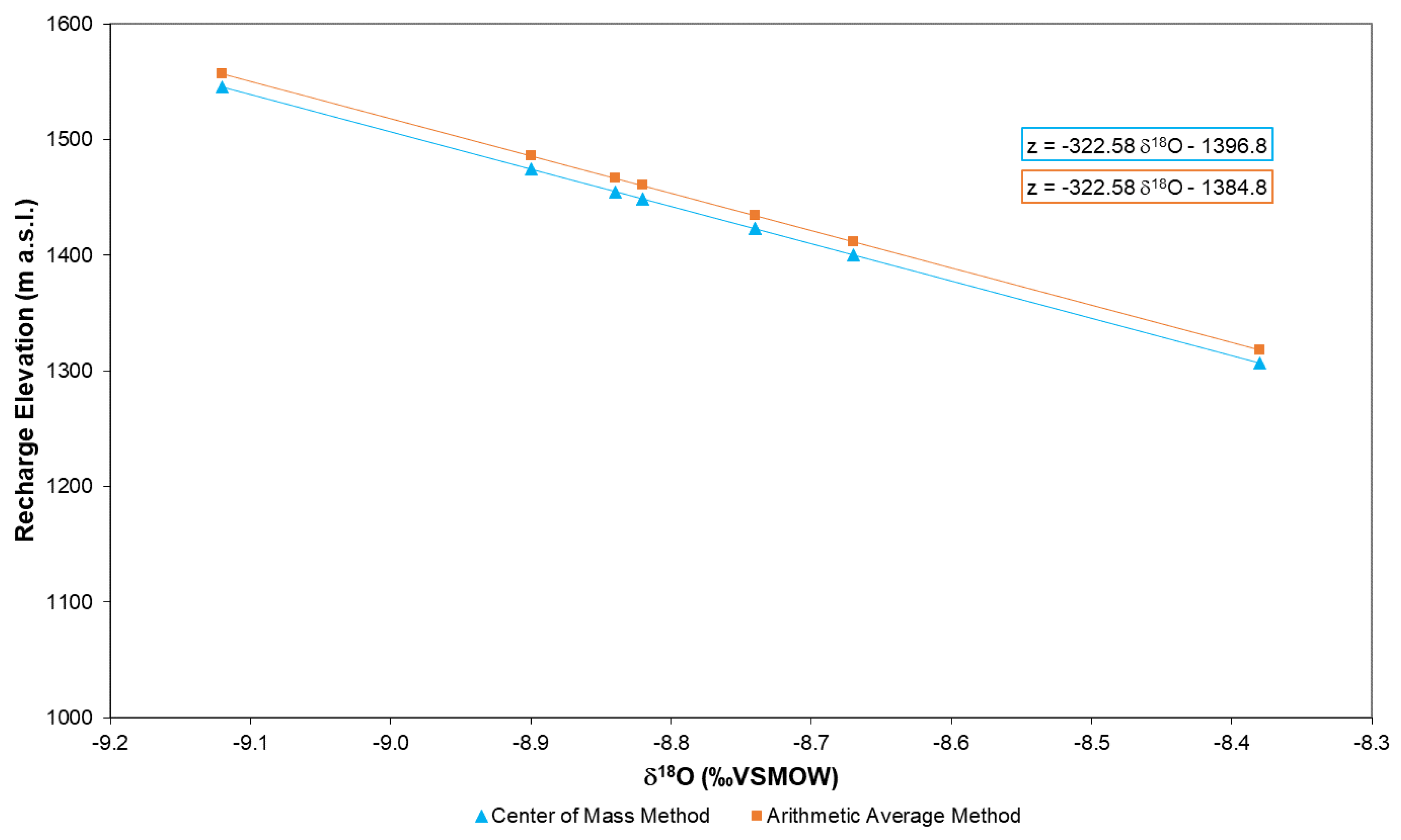
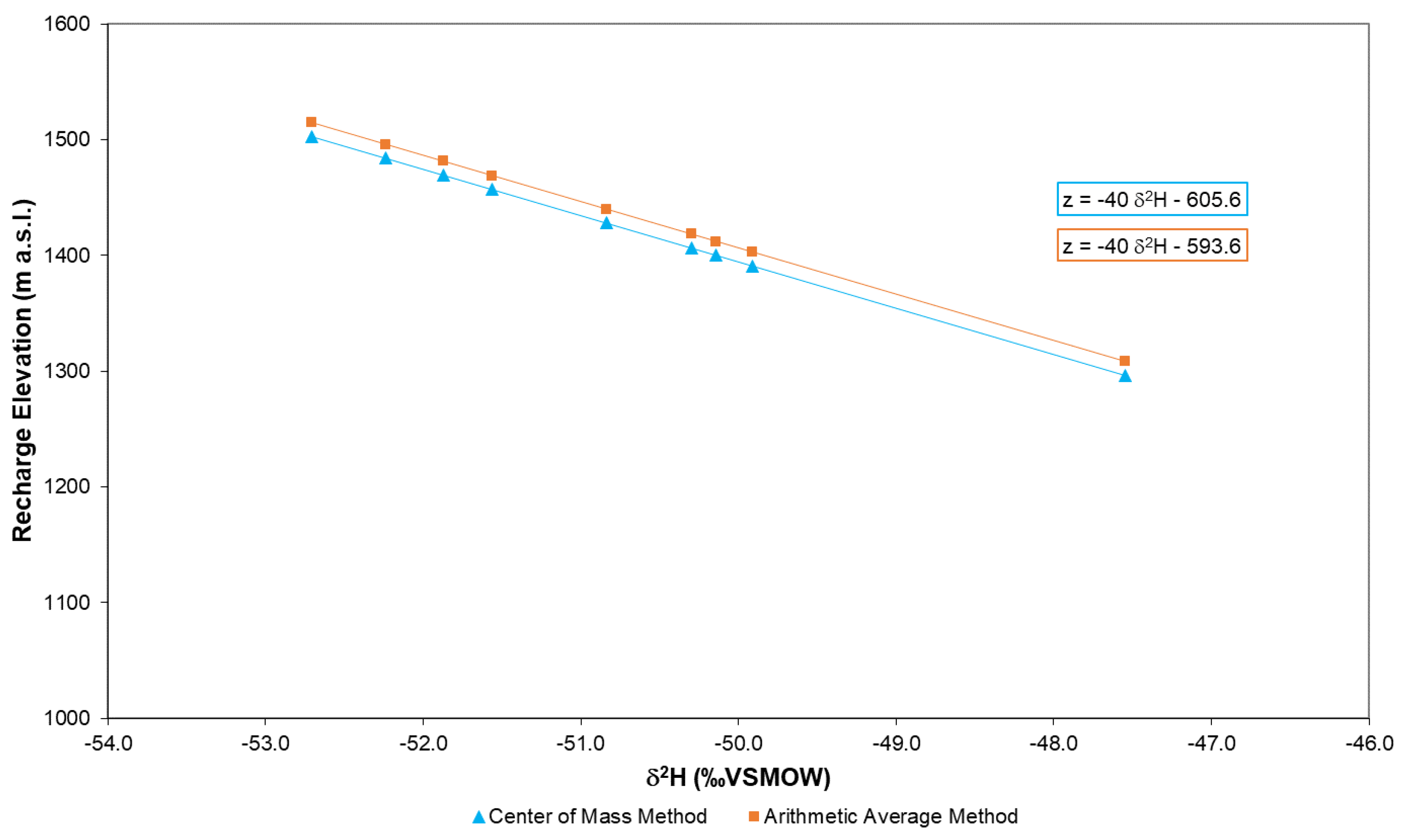
4.2.3. Comparison of Recharge Area Identification Methods

Figure 5 and Figure 6 show the distribution of δ¹⁸O and δ²H values of groundwater samples with respect to recharge elevation obtained by the application of the Center of Mass and Arithmetic Average methods.

The average recharge elevations calculated for the springs show a gradual decrease with increasing recharge elevation. The recharge elevation values obtained by the application of both methods are very similar, and they indicate the accuracy of the relations used.

The obtained recharge elevation values appear to be congruent with the elevations of the hydrogeological basin. With the aim of better verifying the accuracy, the spring recharge elevations were compared with the results of the application of the Inverse Hydrogeological Balance Method, reported in Figure 4. For this reason, the basin has been divided into six elevation classes of 200 m each, and the effective infiltration percentage in each class was calculated (Figure 7).

In the study area, the highest recharge percentage was obtained for the elevation class from 1300 to 1500 m a.s.l. (Figure 7), corresponding very well to the results of the isotopic analysis carried out for the basin. This result is due to the presence of the karst cretaceous limestone outcropping. In a karst framework such as this hydrogeological basin, the presence of highly fractured rocks and, most of all, the specific permeability conditions due to the local karst development processes make the infiltration high and widespread, as confirmed by the general isotopic depletion of groundwater sampled.

The springs’ average recharge elevations, obtained by the application of the Center of Mass Method (1431 m a.s.l.) and the Arithmetic Average Method (1443 m a.s.l.) fall within the class for which the infiltration percentage is highest according to the Inverse Hydrogeological Balance Method (Figure 7). The recharge elevations, obtained for the hydrogeological basin using the two methods described above, are very similar. There is a 1% difference between the values obtained in the two cases.

5. Conclusions

This paper deals with the identification of aquifer recharge areas in a karst basin in Central Italy (Figure 8) using the stable isotope ratios of hydrogen and oxygen combined with the application of the Inverse Hydrogeological Balance Method.

For the Cardellina springs group (GW1, GW2 and GW3), the results show an infiltration area located in the southeast part of the basin at an average elevation of about 1450 m a.s.l. in the Upper Cretaceous carbonates. In contrast, the Cesa degli Angeli spring (GW4) has a higher infiltration elevation than all of the others. This second infiltration area is located in Upper Cretaceous limestone at an elevation of about 1520 m a.s.l. The recharge area of Cornetto (GW5) and Carpinetto (GW6) are located in the northeast part of the basin, at an average elevation of about 1300 and 1400 m a.s.l., respectively. The Pantano springs (GW7, GW8 and GW9) are fed by rainfall, which infiltrates in the western slope of the Assalone Mt, at an elevation of about 1450 m a.s.l. The groundwater isotopic composition of Pantano springs (GW7, GW8 and GW9) is very similar, and as a result, their recharge elevations are very close to one another, highlighting the same infiltration area at an average elevation of about 1450 m a.s.l. in the permeable fractured outcropping of limestone and dolomite.

References

1. Sappa, G.; Ferranti, F.; Ergul, S.; Ioanni, G. Evaluation of the groundwater active recharge trend in the coastal plain of Dar Es Salaam (Tanzania). J. Chem. Pharm. Res. 2013, 5, 548–552. [Google Scholar]
2. Foster, S.; Hirata, R.; Andreo, B. The aquifer pollution vulnerability concept: Aid or impediment in promoting groundwater protection? Hydrogeol. J. 2013, 21, 1389–1392. [Google Scholar] [CrossRef]
3. Bakalowicz, M. Karst groundwater: A challenge for new resources. Hydrogeol. J. 2005, 13, 148–160. [Google Scholar] [CrossRef]
4. Cozma, A.I.; Baciu, C.; Moldovan, M.; Pop, I.C. Using natural tracers to track the groundwater flow in a mining area. Procedia Environ. Sci. 2016, 32, 211–220. [Google Scholar] [CrossRef]
5. Leibundgut, C.; Maloszewski, P.; Kulls, C. Tracer in Hydrology, 1st ed.; Wiley-Blackwell: Chichester, UK, 2009; p. 432. [Google Scholar]
6. Barbieri, M.; Nigro, A.; Petitta, M. Groundwater mixing in the discharge area of San Vittorino Plain (Central Italy): Geochemical characterization and implication for drinking uses. Environ. Earth Sci. 2017, 76, 393. [Google Scholar] [CrossRef]
7. Massmann, G.; Sültenfuß, J.; Dünnbier, U.; Knappe, A.; Taute, T.; Pekdeger, A. Investigation of groundwater residence times during bank filtration in Berlin: A multi-tracer approach. Hydrol. Process. 2008, 22, 788–801. [Google Scholar] [CrossRef]
8. Petitta, M.; Scarascia Mugnozza, G.; Barbieri, M.; Bianchi Fasani, G.; Esposito, C. Hydrodynamic and isotopic investigations for evaluating the mechanisms and amount of groundwater seepage through a rockslide dam. Hydrol. Process. 2010, 24, 3510–3520. [Google Scholar] [CrossRef]
9. Gasser, G.; Pankratov, I.; Elhanany, S.; Glazman, H.; Lev, O. Calculation of wastewater effluent leakage to pristine water sources by the weighted average of multiple tracer approach. Water Resour. Res. 2014, 50, 4269–4282. [Google Scholar] [CrossRef] [Green Version]
10. Moeck, C.; Radny, D.; Popp, A.; Brennwald, M.; Stoll, S.; Auckenthaler, A.; Berg, M.; Schirmer, M. Characterization of a managed aquifer recharge system using multiple tracers. Sci. Total Environ. 2017, 609, 701–714. [Google Scholar] [CrossRef] [PubMed]
11. Nigro, A.; Sappa, G.; Barbieri, M. Application of boron and tritium isotopes for tracing landfill contamination in groundwater. J. Geochem. Explor. 2017, 172, 101–108. [Google Scholar] [CrossRef]
12. Sappa, G.; Ferranti, F.; De Filippi, F.M.; Cardillo, G. Mg2+-based method for the Pertuso spring discharge evaluation. Water 2017, 9, 67. [Google Scholar] [CrossRef]
13. Coplen, T.B.; Herczeg, A.L.; Barnes, C. Isotope engineering—Using stable isotopes of the water molecule to solve practical problems. In Environmental Tracers in Subsurface Hydrology; Cook, P., Herczeg, A.L., Eds.; Kluwer Academic Publishers: South Holland, The Nerthelands, 2000; pp. 79–110. [Google Scholar]
14. Barbieri, M.; Boschetti, T.; Petitta, M.; Tallini, M. Stable Isotopes (2H, 18O and 87Sr/86Sr) and Hydrochemistry Monitoring for Groundwater Hydrodynamics Analysis in a Karst Aquifer (Gran Sasso, Central Italy). Appl. Geochem. 2005, 20, 2063–2081. [Google Scholar] [CrossRef]
15. Sappa, G.; Ergul, S.; Ferranti, F. Water Quality Assessment Of Carbonate Aquifers In Southern Latium Region, Central Italy: A Case Study For Irrigation And Drinking Purposes. Appl. Water Sci. 2014, 4, 115–128. [Google Scholar] [CrossRef]
16. Gat, J.R. Oxygen and hydrogen isotopes in the hydrological cycle. Annu. Rev. Earth Planet. Sci. 1996, 24, 225–262. [Google Scholar] [CrossRef]
17. Rozanski, K.; Araguas-Araguas, L.; Gonfiantini, R. Isotopic patterns in modern global precipitation. In Climate Change in Continental Isotopic Records; Swart, P.K., Lohmann, K.C., McKenzie, J., Savin, S., Eds.; American Geophysical Union: Washington, DC, USA, 1993; Volume 78, pp. 1–36. [Google Scholar]
18. Song, C.; Wang, G.; Liu, G.; Mao, T.; Sun, X.; Chen, X. Stable isotope variations of precipitation and streamflow reveal the young water fraction of a permafrost watershed. Hydrol. Process. 2017, 31, 935–947. [Google Scholar] [CrossRef]
19. Kirchner, J.W. Aggregation in environmental systems-Part 1: Seasonal tracer cycles quantify young water fractions, but not mean transit times, in spatially heterogeneous catchments. Hydrol. Earth Syst. Sci. 2016, 20, 279–297. [Google Scholar] [CrossRef]
20. Dansgaard, W. Stable isotopes in precipitation. Tellus 1964, XVI, 436–468. [Google Scholar]
21. Gat, J.R.; Gonfiantini, R. Stable Isotope Hydrology. Deuterium and Oxygen-18 in the Water Cycle; Series No. 210; Technical Reports for International Atomic Energy Agency (IAEA): Vienna, Austria, 1981; p. 356. [Google Scholar]
22. Gonfiantini, R.; Roche, M.-A.; Olivry, J.-C.; Fontes, J.-C.; Zuppi, G.M. The altitude effect on the isotopic composition of tropical rains. Chem. Geol. 2001, 181, 147–167. [Google Scholar] [CrossRef]
23. Craig, H. Isotopic variations in meteoric waters. Science 1961, 133, 1702–1703. [Google Scholar] [CrossRef] [PubMed]
24. Clark, I.D.; Fritz, P. Environmental Isotopes in Hydrogeology; CRC Press/Lewis Publishers: Palm Beach County, FL, USA, 1997; p. 342. [Google Scholar]
25. Civita, M.; De Maio, M. Average Groundwater Recharge in Carbonate Aquifers: A GIS Processed Numerical Model. In Proceedings of the VII Conference on Limestone Hydrology and Fissured Media, Besancon, France, 20–22 September 2001; Université de Franche-Comté, Sciences & Techniques de l’Environnement: Besançon, France, 2001. [Google Scholar]
26. Devoto, G. Note Geologiche Sul Settore Centrale Dei Monti Simbruini Ed Ernici (Lazio Nord-Orientale); Stabilimento Tipografico G. Genovese: Naples, Italy, 1967; pp. 1–112. [Google Scholar]
27. Devoto, G. Sguardo geologico dei Monti Simbruini (Lazio nord-orientale). Geol. Rom. 1970, 9, 127–136. [Google Scholar]
28. Devoto, G.; Parotto, M. Note geologiche sui rilievi tra Monte Crepacuore e Monte Ortara (Monti Ernici-Lazio nord-orientale). Geol. Rom. 1967, 6, 145–163. [Google Scholar]
29. Accordi, G.; Carbone, F. Sequenze carbonatiche meso-cenozoiche. Note illustrative alla Carta delle Litofacies del Lazio-Abruzzo ed aree limitrofe. Quad. Ric. Scient. 1988, 114, 11–92. [Google Scholar]
30. Damiani, A.V. Studi sulla piattaforma laziale-abruzzese. Nota I. Considerazioni e problematiche sull’assetto tettonico e sulla paleogeologia dei Monti Simbruini. In Memorie. Della Descrittive Carta Geologica D’Italia; Istituto Superiore per la Protezione e la Ricerca Ambientale: Roma, Italy, 1990; Volume 38, pp. 145–176. [Google Scholar]
31. Bono, P.; Percopo, C. Flow dynamics and erosion rate of a representative karst basin (Upper Aniene River, Central Italy). Environ. Geol. 1996, 27, 210–218. [Google Scholar] [CrossRef]
32. Ventriglia, U. Idrogeologia della Provincia di Roma, IV, Regione Orientale. In Hydrogeology of the Province of Rome, IV, Eastern Region; Amministrazione provinciale di Roma: Roma, Italy, 1990. [Google Scholar]
33. Penta, F. Indagini Nella Zona delle Sorgenti del Simbrivio, Istituto di Giacimenti Minerari e Geologia Applicata; Sapienza University of Rome: Roma, Italy, 1956. [Google Scholar]
34. Sappa, G.; Ferranti, F. An integrated approach to the Environmental Monitoring Plan of the Pertuso Spring (Upper Valley of Aniene River). Ital. J. Groundw. 2014, 3, 47–55. [Google Scholar] [CrossRef]
35. White, W.B. Geomorphology and Hydrology of Karst Terrains; Oxford University Press: New York, NY, USA, 1988. [Google Scholar]
36. White, W.B. Karst hydrology: recent developments and open questions. Eng. Geol. 2002, 65, 85–105. [Google Scholar] [CrossRef]
37. Longinelli, A.; Selmo, E. Isotopic Composition of Precipitation in Italy: A First Overall Map. J. Hydrol. 2003, 270, 75–88. [Google Scholar]
38. Gourcy, L.L.; Groening, M.; Aggarwal, P.K. Stable oxygen and hydrogen isotopes in precipitation. In Isotopes in the Water Cycle: Past, Present and Future of Developing Science; Aggarwal, P.K., Gat, J.R., Froehlich, K.F.O., Eds.; Springer: Dordrecht, The Netherlands, 2005; pp. 39–51. [Google Scholar]
39. Gat, J.R.; Carmi, I. Evolution of the isotopic composition of atmospheric waters in the Mediterranean Sea Area. J. Geophys. Res. 1970, 75, 3039–3048. [Google Scholar] [CrossRef]
40. Cappa, C.D.; Hendricks, M.B.; DePaolo, D.J.; Cohen, R.C. Isotopic fractionation of water during evaporation. J. Geophys. Res. 2003, 108, D16. [Google Scholar] [CrossRef]
41. Gat, J.R.; Matsui, E. Atmospheric water balance in the Amazon Basin: an isotopic evapotranspiration model. J. Geophys. Res. Atmos. 1991, 96, 13179–13188. [Google Scholar] [CrossRef]
42. Cox, K.A.; Rohling, E.J.; Schmidt, G.A.; Schiebel, R.; Bacon, S.; Winter, D.A.; Bolshaw, M.; Spero, H.J. New constraints on the Eastern Mediterranean δ18O:δD relationship. Ocean Sci. Discuss. 2011, 1, 39–53. [Google Scholar] [CrossRef] [Green Version]
43. Gat, J.R.; Klein, B.; Kushnir, Y.; Roether, W.; Wernli, H.; Yam, R.; Shemesh, A. Isotope composition of air moisture over the Mediterranean Sea: an index of the air-sea interaction pattern. Tellus B Chem. Phys. Meteorol. 2003, 55, 953–965. [Google Scholar] [CrossRef]
44. Bortolami, G.C.; Ricci, B.; Susella, G.F.; Zuppi, G.M. Isotope hydrology of the Val Corsaglia, Maritime Alps, Piedmont, Italy. In Isotope Hydrology; International Atomic Energy Agency IAEA: Vienna, Austria, 1978; pp. 27–350. [Google Scholar]
Figure 1. Geological map of the study area and location of karst basin.
Geosciences 08 00351 g001
Figure 2. Plot of δ2H vs. δ18O for spring water samples collected in June 1997 and October 2002 with (GLMM): Global Meteoric Water Line [38], (MLML): Mediterranean Meteoric Water Line [39], (CILML): Central Italy Meteoric Water Line [37].
Geosciences 08 00351 g002
Figure 3. Monthly average rainfall and Carpinetto spring (GW6), average rate.
Geosciences 08 00351 g003
Figure 4. Average annual active evaluate using the Inverse Hydrogeological Balance Water Method (a) FSE, (b) interpolation.
Geosciences 08 00351 g004
Figure 5. δ18O values of spring samples plotted against recharge elevations (October 2002).
Geosciences 08 00351 g005
Figure 6. δ2H values of spring samples plotted against recharge elevations (October 2002).
Geosciences 08 00351 g006
Figure 7. Bar plot of effective infiltration (%).
Geosciences 08 00351 g007
Figure 8. Hydrogeological basin recharge areas and groundwater flowpaths.
Geosciences 08 00351 g008