Abstract
A range of data sources are now used to support the process of archaeological prospection, including remote sensed imagery, spy satellite photographs and aerial photographs. This paper advocates the value and importance of a hitherto under-utilised historical mapping resource—the Survey of India 1” to 1-mile map series, which was based on surveys started in the mid–late nineteenth century, and published progressively from the early twentieth century AD. These maps present a systematic documentation of the topography of the British dominions in the South Asian Subcontinent. Incidentally, they also documented the locations, the height and area of thousands of elevated mounds that were visible in the landscape at the time that the surveys were carried out, but have typically since been either damaged or destroyed by the expansion of irrigation agriculture and urbanism. Subsequent reanalysis has revealed that many of these mounds were actually the remains of ancient settlements. The digitisation and analysis of these historic maps thus creates a unique opportunity for gaining insight into the landscape archaeology of South Asia. This paper reviews the context within which these historical maps were created, presents a method for georeferencing them, and reviews the symbology that was used to represent elevated mound features that have the potential to be archaeological sites. This paper should be read in conjunction with the paper by Arnau Garcia et al. in the same issue of Geosciences, which implements a research programme combining historical maps and a range of remote sensing approaches to reconstruct historical landscape dynamics in the Indus River Basin.
1. Introduction
Landscape archaeology is fundamentally concerned with recording of the distribution of ancient settlement and the environments within which they were situated, and makes use of a range of different sources of data to aid the multi-faceted and multi-phased process of landscape prospection [1]. Remote assessment is important for directing effective survey on the ground, but it also provides insight into the distribution of archaeological sites in areas and/or regions that are otherwise inaccessible (e.g., areas of Afghanistan [2,3,4,5]; Syria [6]; Thessaly [7]). Satellite imagery and aerial photography now play an indispensable role in the landscape archaeology of many regions, but their usefulness is curtailed by their relatively restricted time depth. In contrast, for some parts of the world there are historical map series that document the landscape long before major intensive agricultural practices and development programmes removed heretofore preserved vestiges of past landscapes. These historic maps provide an important additional source of data for landscape archaeology that is complementary to remote sensing imagery and aerial photography, and has a similar but relatively under-utilised potential to generate major new insights into past landscapes. This paper argues that the digitisation and analysis of historic maps has unique potential for the landscape archaeology of South Asia, where there are a range of historical map resources and modern development has profoundly obscured complex archaeological landscapes.
The Survey of India 1” to 1-mile (1:63,360 scale) map series originated in a very specific imperial context [8], and were based on surveys carried out from the mid–late nineteenth century onwards. These surveys were started in the wake of the conquest of Punjab and the then North-West Frontier Province and the Indian rebellion of 1857, which is also known as the First War of Independence. The resulting maps were published from the early twentieth century onward as part of series that were issued progressively and updated incrementally, and they were primarily designed to present information that was relevant to the military, such as the location of villages, roads, irrigation canals and the nature of land-use [9]. The surveys and the maps they produced also incidentally documented the locations and, to some extent, the height and area, of thousands of elevated mounds that were visible in the landscape at the time that the surveys were carried out. It appears that in most instances the surveyors did not recognise these mounds as anything unusual. A significant proportion of these mounds were actually the remains of ancient settlements, some of which built up during the processes of the formation and abandonment of ancient settlements millennia ago.
While archaeologists have long been aware of the potential of the Survey of India 1” to 1-mile maps, and made use of them as early as the late 1940s/early 1950s [10], their use has been limited in terms of the areal extent. J.R. Knox carried out a systematic assessment of a significant number of map sheets as part of graduate research in the 1970s, but these maps have not been used to guide more recent archaeological surveys or as a data source in combination with remote sensing data. As such, the significance of these maps as a data source for large-scale systematic mapping of archaeological sites has not been explored. This paper considers the historical context within which the Survey of India 1” to 1-mile map series was created, its incidental documentation of archaeological sites, and the degree to which surveyors knew what they were recording. To highlight the utility of this rich data source, this paper also outlines a systematic method for (a) georeferencing these maps and (b) identifies symbols that represent features and/or archaeological site locations.
2. Reconstructing Archaeological Landscapes Remotely
The declassification of spy satellite photographs (e.g., CORONA, GAMBIT, HEXAGON keyhole series) and the availability of Open Access remote sensing data (e.g., Landsat, Aster, Copernicus; [1,11,12]) has meant that a wide range of imaging system data sources are now used (both extensively and intensively) for prospection. Furthermore, a substantial (and growing) body of literature now highlights the importance of historic satellite and remote sensing imagery for documenting ancient landforms and settlements, particularly those at risk of being modified, obscured and/or obliterated in the process of modern urban and rural development [1,3,4,5,13,14,15,16,17,18,19,20,21,22,23,24,25,26,27,28,29,30,31,32,33,34,35,36,37].
Such high-resolution imagery has had a profound impact upon archaeological knowledge, but it does have limitations. Declassified spy satellite imagery only post-dates the 1950s and though it saw markedly improved resolution in the 1970s [1], it has issues with distortion [38]. Furthermore, not all parts of the world have coverage, let alone high-quality coverage, as much spy satellite imagery acquisition focused on geopolitical “hot spots”. While China, the former USSR, and parts of the Middle East are covered extensively in US imagery, and Soviet imagery covered parts of Europe, imagery for other areas is either poor or non-existent. Coverage for much readily available remote sensing imagery is global, but is often limited in terms of its resolution and chronological range, which means that many features are not visible because the imagery was acquired after instances of modern disturbance [1,15].
The use of aerial photography for archaeology has a long history, beginning with the use of balloons in the nineteenth century and being advanced through the methods of reconnaissance and documentation using aeroplanes developed during the First World War [1,39,40]. Aerial archaeology in many parts of the world is now well developed (e.g., UK, USA, France, Italy, Jordan), and important historic imagery is available via substantial archives (e.g., National Collection of Aerial Photography, which contains images from the UK and much of the world). Historic aerial photos provide an invaluable record of many landscapes before they were disturbed by modern activities, and our understanding of the archaeology of some regions has been completely transformed through their use (e.g., Jordan; [1,7,40,41,42,43,44]). In relative terms, however, aerial photo coverage is again limited and/or unsystematic. Vertical and oblique images also have specific advantages and disadvantages related to distortion and visibility of features, with the latter being affected the timing of the photographs (time of day and time of year etc. [45,46,47,48]).
Maps have a longer history, and thus considerable potential for documenting lost or disappearing landscapes. While early maps contain limited topographic information and lack accuracy, the information documented by mapping projects in various nation states and former imperial dominions from the eighteenth and nineteenth century AD onwards was of a different order of accuracy due to advances in methods and the scale of the endeavour. Starting from the Cassini maps of France and the maps created of the UK prior to the establishment of the Ordnance Survey, surveyors set out to document landscapes and topography systematically. As these maps were created at particular points in time, it is also possible to monitor change in landscape over time by comparing different maps, particularly where individual maps are updated and reissued [49]. The maps produced by these systematic surveying projects have considerable potential for documenting archaeological sites, and it is notable that in the UK, there was clear interaction between the Ordnance Survey and the various Royal Commissions for Historic Monuments, such that easily visible archaeological sites are clearly marked on the maps and their legends [49,50].
There is growing interest in the history and execution of the mapping projects carried out in various imperial dominions, particularly those of the UK [8,51,52,53,54], but also the former USSR. The inclusion of archaeological sites on Soviet era maps of parts of the former USSR and Afghanistan produced by the Soviet Military Topographic Service has been noted [5,28,55], but these maps have been used in relatively limited areas and/or on a relatively small scale. It is notable that the types of sites that are easy to distinguish on these maps are clearly ancient sites with distinctive morphologies.
3. Mapping Territory and Surveying Archaeology: The Survey of India, the Archaeological Survey of India, and the 1” to 1-Mile Map Series
3.1. Systematic Mapping in Nation States and Imperial Dominions: Trigonometry, Topography and Archaeology
The mapping of nation states and imperial dominions is a deeply political act, typically intertwined with military objectives. For instance, the roots of the UK’s Ordnance Survey lie in the commencement of a systematic attempt to map the highlands of Scotland in 1747 after the Jacobite rising [49,56]. The establishment of the Survey of India soon followed in 1767 [51,52,57,58,59]. These august institutions are probably best seen as siblings—developed in parallel by government agencies that were interacting, and with objectives and innovations being transferred quickly between the two.
Accurate mapping soon became a key objective, and the Principal Triangulation of Britain, carried out between 1791 and 1853, was the first high-precision trigonometric survey of the whole of Great Britain and Ireland [56,59]. Shortly thereafter, the Great Trigonometrical Survey (GTS) set out to complete the more formidable task of measuring the entire South Asian Subcontinent between 1802 and 1871 [51,52]. This work of the GTS was inherently scientific and profoundly significant, but in many ways, it was controversial, particularly its cost in life and materials [51]. It nonetheless provided the framework for the more detailed mapping of topography that started 1831 [8,51], and was accompanied by the Revenue Survey, and occurred concurrently with the compilation of the Gazetteers of British India: District Series (1833 onwards [60]) and The Imperial Gazetteer of India [61].
The history of the Survey of India is a rich vein for scholarly enquiry, particularly as it was extensively documented [57,58,62,63,64]. Beyond consideration of its contribution to geodesy and cartography, it is ripe for the deconstruction of imperial ideology, the political impact of map making, and the conception of borders and frontiers [8,51,52,53]. Most scholarly attention has been directed to the period before 1843, which Edney [51], also [8] has referred to as a phase of “cartographic anarchy”, when colonial surveyors struggled with the practical complications and epistemological challenges of surveying such extensive and (geographically and culturally) complex territory. In contrast, the period from 1843 to 1904 is regarded as one of consolidation and comprehensive survey [52,57,58], which was marked by progressive expansion of the territory controlled by the colonial authorities and the implementation of measures to systematically document the subcontinent district by district (see above).
The Survey of India 1” to 1-mile maps (Figure 1, Figure 2 and Figure 3) were intended to document the landscape of British dominions in the Subcontinent systematically, and there are also 1” to 2-mile and 1” to 4-mile series. Complaints from the military authorities in 1905 resulted in the establishment of a committee to formulate a policy on map production to meet military and civil needs, and this Committee of 1905–06 devised a specific layout for these maps using contours and colours that continued in use up until the Second World War when the civil survey and publication programme was curtailed [57,58]. Comprehensive historical information about the progress of the survey and the publication of the 1” to 1-mile and associated series is restricted and not yet in the public domain. These maps were, however, issued on the basis of a grid of quadrangles that spanned the entire South Asian subcontinent and the surrounding regions (Figure 2).
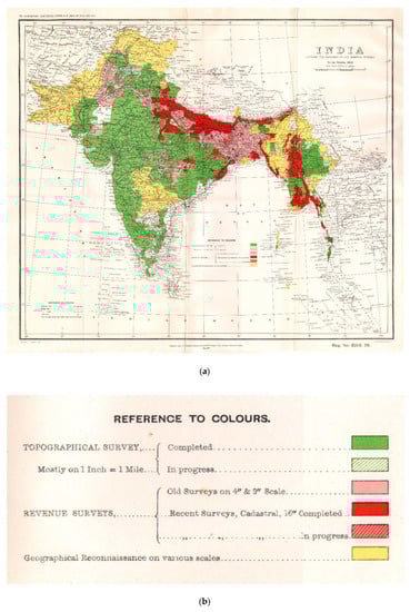
Figure 1.
(a) Map showing progress of imperial surveys up to 1st October 1904 (Image: Pahar.in; Public Domain [66]). (b) Close-up of the legend from the same map (Image: Pahar.in; Public Domain [66]).
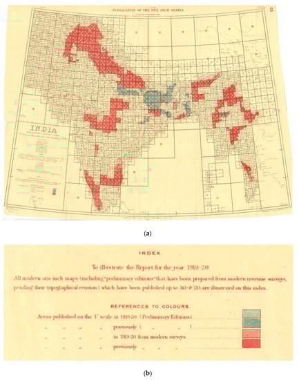
Figure 2.
(a) Map showing structure of 1” to 1-mile map series and its publication as at 1920 (Image: Pahar.in; Public Domain [66]). (b) Close-up of the legend from the same map (Image: Pahar.in; Public Domain [66]).
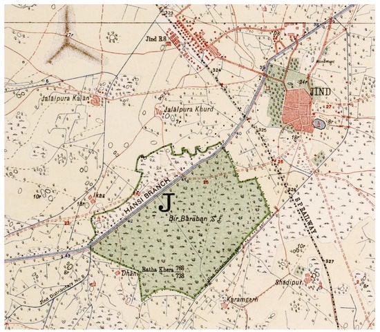
Figure 3.
Detail from 1” to 1-mile map sheet 53/C7/1915, showing the types and range of information being documented (e.g., built-up areas, railways, roads, ponds, irrigation canals, cultivated areas, forest, temples) (Image courtesy of Cambridge University Library).
The production of these maps in the early twentieth century occurred on the back of the topographic surveys that had started over 50 years before, and whose execution was documented in two editions of The Manual of Surveying in India [9,65]. The importance of these maps for both administrative and military purposes meant that specific guidance was given for the types of features that were essential to document, particularly rivers, streams, canals, populated areas, roads and areas suitable for military camps or positions ([9], pp. 441–448). As Thuillier and Smyth ([9], p. 281) noted “The conspicuous objects and all geographical items thus laid down, but all the different descriptions of land separated, viz. cultivation, waste, fallow, sites of villages and land fit for cultivation, the area of which being required for settlement purposes, is found by triangulation on the map”. The geographical and topographic features were supposed to be documented using the same system and/or a consistent set of principles, and reference was made to a number of core European military surveying manuals ([9], p. 285).
Specific choices were made about line style and thickness to ensure that photography could be used for reproducing the maps, and certain types of land were not mapped, including plots of barren waste and jungle of less than 40 acres in area ([9], p. 312). For reasons that will become clear below, it is notable that specific guidelines were in place for documenting hills and elevated areas, and reference was made to ‘vertical’ and ‘horizontal’ styles:
“In the first method the shade is formed by strokes of the pencil or pen radiating from or converging into any curved part of a hill, according as it projects or re-enters:—they are supposed to describe the same course as water would do, if it would trickle in streams down the slopes, and are darker or lighter according to the steepness of the slope. The other method has the shade formed by lines parallel, or nearly so, to the horizon. It is much more easy to apply, and more natural than the former, and has some claim to particular notice from its easy application in sketching, and the facility with which it may be demonstrated and acquired. The horizontal manner marks the contours of hills by waving lines, each line continuing on the same level, while following every undulation of the ground. In practice, either or both of the styles may be used at the pleasure of the draftsman, or as may be best suited to the nature of the ground he wishes to portray”([9], pp. 297–300)
Surveyors were thus granted a degree of agency in how they chose to depict hills or elevated ground, and they presumably adapted their symbology to suit the needs of depicting elevations on the relatively flat plains that predominate in many areas. Accuracy and precision were nonetheless critical, and “hilly features should invariably be put in, by the Surveyor himself, after a careful study of the ground, and without this personal examination in the field, it must be vain to attempt to give even an approximation to truth. It is evident that a map, to be anything, ought to be precise; it is otherwise worse than useless” ([9], p. 300).
During the period in which the systematic topographic mapping of the subcontinent was underway, Colonel Alexander Cunningham was appointed as the Archaeological Surveyor of the Government of India in November 1861. Cunningham had made the case that the government was honour bound to understand and preserve the ancient monuments of the British dominions in India. He argued that they must be “preserved by the accurate drawings and faithful descriptions of the archaeologist”, and that it “would redound equally to the honour of the British Government to institute a careful and systematic investigation of all existing monuments of ancient India” ([67], pp. iii, iv). It is notable that the Archaeological Survey of India (ASI) was established over twenty years before the UK’s Ancient Monuments Protection Act 1882, and 47 years before the various Royal Commissions on the Historic Monuments of Scotland, Wales and England (1908).
A major limitation of the early work of the ASI under Cunningham was that he and his subordinates largely documented settlements that were known from historical documents. Cunningham ([67], p. iv; [68], pp. xxi–xxxiv) started by following in the footsteps of the Chinese pilgrim Xuanzang, who travelled throughout South Asia in the seventh century AD. Cunningham also took account of other ‘foreign’ accounts of South Asia made by other Chinese pilgrims (e.g., Faxian, Song Yun), and the works of the Alexander historians (Arrian, Quintus Curtius) and their followers (Strabo, Pliny the elder, Ptolemy etc.). Furthermore, he also made use of the range of indigenous sources in various forms, including Vedic texts and the epic Ramayana and Mahabharata, as well sutras and astronomical works ([68], pp. xxxiv–lii). These approaches were paralleled in Arabia and the Levant, where the documentation of archaeological sites mentioned in the Bible, Classical, and Mesopotamian sources was a clear objective of the surveying that was carried out under the influence of the Survey of India ([54], pp. 42, 64, 113).
3.2. Parallel Developments in the Ordnance Survey and the Survey of India
Given that the ASI set out to complete a “systematic investigation of all existing monuments of ancient India”, it is instructive to consider the interconnection between the work of the ASI and that of the Survey of India. It is also important to consider contemporary developments in the mapping of archaeological sites that were taking place elsewhere.
The early twentieth century Ordnance Survey maps of the UK typically documented visible archaeological features such as earthworks and tumuli [50,69,70]. There were, however, several occasions (e.g., Haverfield’s 1906 lecture to the Royal Geographical Society on Hadrian’s Wall) when it was made clear that there was a disconnect between the work of the Ordnance Survey and their depiction of archaeological sites on maps, and the professional knowledge of the archaeology that was being depicted ([50], pp. 22–23; [71]). Major change in the mapping of ancient sites in the UK only occurred when OGS Crawford (who was, interestingly, born in India) was appointed the first Archaeology Officer of the Ordnance Survey in 1920 ([50], p. 23). It is also notable that during this period, an Empire Conference of Survey Officers was inaugurated to bring together surveyors from across the British Empire [71,72], and it was just before the second event that Crawford [73] published a paper on mapping ‘primitive English landmarks’. Survey of India representatives were present at the first Empire Conference [74], and it is almost certain that Crawford’s paper would have been read by representatives of the Survey of India. Although knowledge of archaeology in the UK increased exponentially during the twentieth century, it is notable that the majority of what is now depicted on maps are features visible above the ground, and subtle and/or sub-surface features are not typically displayed. In the UK context, such subtle features make up a substantial proportion of the preserved archaeological landscape, which has effectively left them ‘invisible’ on maps, even though they are well understood through the extensive use of aerial archaeology and geophysical prospecting.
While a substantial proportion of the archaeology in the UK is not visible on the surface, this is not the case for much of the Subcontinent. Much like areas in the ancient Near East, ancient settlements in India and Pakistan were typically made of mud-brick or fired brick, resulting in the creation of mounded sites. Such sites often have variations of local terms in their names that reflect that fact (e.g., khera, tibba, tibbi, tepe, tul, theh, tol, tell), and there are instances where such features are labelled on maps (e.g., Ratha Khera, which is indicated on Figure 4, and is also the location of a trigonometric point). There were almost certainly other types of archaeological sites that do not preserve as mounds, but mounds are the most visible type of archaeological remains.
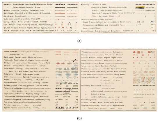
Figure 4.
(a) Reproduction of legend from a 1915 map (53/C3/1915); (b) Reproduction of legend from a 1936 map (53/D9/1936) (Images courtesy of Cambridge University Library).
3.3. Incidental Documentation of Archaeology in the Survey of India 1” to 1-Mile Maps
There has been a long tradition of archaeological survey in South Asia, which has recorded numerous site locations [75,76,77,78]. While substantial numbers of ‘proto-historic’ sites are now known, up until the large scale survey projects started in the 1970s, the extent of the distribution of these elevated mounds was largely unrecognised. Of the large number of settlements now known to relate to the Indus Civilisation (c.3000–1500 BC), for example, it is notable that only the ancient city at Harappa was known in the initial period of topographic survey in the nineteenth century AD, and that was largely because it had been described by Charles Masson and Alexander Burnes in the earlier nineteenth century ([79], p. 6). Rather than being able to conceive that this mound might be pre- or proto-historic in date, Cunningham ([68], p. 241) suggested that it may have been the location of “another city of the Malii” mentioned by Arrian. A number of other early Indus settlements were also discovered at that time (e.g., Sutkagen-dor, Dabar Kot, Periano Ghundai, Rana Ghundai ([76], pp. 53–56), but they are situated in areas that were only subjected to preliminary reconnaissance or low-resolution survey prior to the Second World War.
There was some general awareness amongst the surveyors of the Survey of India of major archaeological sites, as the Survey of India 1” to 1-mile series maps document the archaeological sites that had been documented by the Archaeological Survey of India and/or were known at the time of the production of the maps of the during the early decades of the twentieth century. There appears to have been a consistent approach to the symbology that was used to depict the mound sites, which was presumably a result of the actions of the Committee of 1905–06. There was, however, a degree of evolution in the way that legends were depicted, with specific differences evident in maps from 1915 (Figure 4a) and those from 1936 (Figure 4b), where ‘Antiquities’ are indicated at the top right of the latter. These same differences are evident in the legends of the Ordnance Survey maps from the same period. Such sites are indicated on the maps through the use of gothic script (e.g., Harapâ [80], pp. 105–108); Sites of Ancient Cities of Harappa, 44/B14/1936; Figure 5a), which is again something that appears in Ordnance Survey maps of the same period and up to the present. Furthermore, archaeological sites are mentioned in a number of District Gazetteers, and the Director General of the ASI and other subordinates are thanked for providing relevant information [81]. Significantly, the well-known archaeological sites that were comprised of elevated mounds were not typically depicted through the use of contours, but through the use of ‘form-lines’, which are ‘lines drawn on a map to indicate the estimated configuration or elevation between the contour lines’ (Oxford English Dictionary) (Figure 5a). Furthermore, elevated mounds that were not then known as archaeological sites, including the major Indus Civilisation city of Rakhigarhi, were also documented using ‘form lines’ (Figure 6a). Although there has been considerable development adjacent to both sites, they are still visible in modern satellite photos (Figure 5b and Figure 6b).
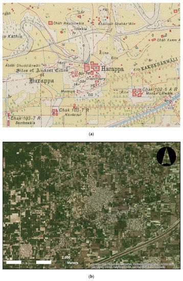
Figure 5.
(a) Detail showing documentation of the “Sites of Ancient Cities of Harappa”, including depiction of mounds delineated by ‘form-lines’, graves, and ‘x’ signifying deserted villages, and their relationship to the modern town (44/B14/1933) (Image courtesy of Cambridge University Library); (b) ESRI world imagery of the same region today.
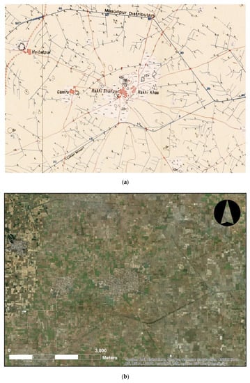
Figure 6.
(a) Detail showing documentation of mounds of the Indus city of Rakhigarhi and their relationship to the modern towns of Rakhi Shapur and Rakhi Khas (53/C3/1915) (Image courtesy of Cambridge University Library); (b) ESRI world imagery of the same region today.
Examination of a selection of Survey of India 1” to 1-mile maps from the region of northwest India has shown that a range of symbols were used to depict the elevated ground that has the potential to be archaeological mound sites. In addition to ‘form-lines’, these symbols include ‘sand-hills’ (either ‘surveyed’ or ‘conventional’), vertical hachures, which are not shown on the standard legend, and also areas of ‘graves’, which are often visible on top of areas indicated with ‘form-lines’ (Figure 4b). These graves are typically historic and/or contemporary Muslim cemeteries and not particularly ancient. There is also a distinctive ‘X’ symbol used to depict ‘deserted villages’, and these are sometimes accompanied by a note stipulating ‘(old site)’—which have been observed on the 1” to 1-mile maps sheets for Gujarat, and are also seen on the 1955 US Topo Map series, which were based on the Survey of India maps and produced in black-and-white.
Although the work of the Survey of India in the early twentieth century was taking place at an enormous scale and with considerable speed, the work was systematic and the survey methods that were used resulted in the incidental location and documentation of thousands of features that may have an archaeological origin. As far as we can ascertain, it is likely that the surveying teams, and the administrators who superintended them, had limited to no awareness of the archaeological significance of these small, elevated features that were being recorded with considerable fidelity. However, it is notable that Rondelli et al. [28] have argued that Soviet surveyors knew that they were documenting archaeological sites when they were working in Central Asia. The Survey of India currently regards the sites marked with an ‘X’ as being “A site that was inhabited in the past, but found uninhabited during field survey” (Surveyor General of India, personal communication 2015). It is thus possible that the Survey of India teams had a vague awareness that what they were documenting was historically significant.
Irrespective of whether the surveyors knew that they were recording archaeological sites, it is clear that the Survey of India 1” to 1-mile maps provide a major data source for identifying and locating mound shaped features that might be archaeological mound sites in advance of on-the-ground survey projects. There are however, a number of challenges and limitations to using this resource, and to overcome these we have developed methods to (a) geo-reference the 1” to 1-mile maps accurately, and (b) extract location information that can be ground-truthed to assess whether or not an archaeological site is present and ascertain its date.
4. Geo-Referencing Survey of India 1” to 1-Mile Maps
In order to make use of the Survey of India 1” to 1-mile maps as a prospecting resource we have established methods for georeferenciation using both ArcMap and QGIS georeferenciation tools (a plugin using GDAL in the case of QGIS). The maps themselves, and the processes of reproduction, were comparably accurate with the Ordnance Survey maps of the same period, and likely used the Everest 1830 spheroid. They were, nonetheless, printed on paper and have also subsequently been held in library collections where they are often folded, which creates the potential for distortion, particularly in digitisation processes that involve photography or scanning, and both of these can also introduce distortion. All of these factors affect the process of georeferenciation.
Using WGS84 as the geodetic datum, the first step in the georeferenciation process consisted of the selection of two points from opposite corners at the graticule of meridians and parallels available at the frame of the map (the corner of the map frames are always coincidental with every 15 minutes on a lat/long grid, so each map covers ¼ of a degree). The coordinate values of these points transformed to decimal degrees were then inserted manually into the georeferenciation tool. These steps produced a rough initial georeferenciation that made it possible to scale, orientate and situate the map in its approximate geographical location. It is notable that the use of coordinates from the map graticule (even when employing four or six points geometrically distributed) were not accurate enough when compared with independently geo-referenced imagery, and produced large deviations across the map. After this first step, a georeferenciation method using target data from an already georeferenced source was adopted. Typically, ground control points (GCPs) were obtained in ArcGIS and QGIS using their world imagery map services. Both feature high-resolution aerial imagery that can be employed to identify features that were extant at the time that the initial surveying for the maps was carried out.
A minimum of 20 GCPs distributed evenly across each map was considered necessary for a reliable georeferenciation. GCPs were obtained from clearly delimited structures and features visible on each map sheet and modern remote sensing imagery, particularly canals, old structures and intersections in villages. Given the degree of modifications that have affected the whole of the study during the last hundred years and the scale of the maps, it was often difficult to find reliable GCPs. Many elements of the landscape have disappeared since the late nineteenth century AD, and most urban areas have changed dramatically, such that their layout as shown in the maps is no longer recognisable. The most useful elements for the retrieval of GCPs were crossings within the water channel network. Channels were carefully mapped during the nineteenth century AD, due to a combination of their lineal nature, the detailed surveying that went into their construction, and the core objectives of the original surveys, all of which mean that they are a source of reliable GCPs. Much of the large network of channels that is still being used has existed since the late nineteenth and early twentieth centuries, including many crossings and junctions. These offer well-distributed and reliable GCPs that can be correlated to the features still preserved today that are clearly visible and easy to identify in high-resolution aerial and satellite imagery. For similar reasons regional roads and railroads were preferred elements for the extraction of GCPs. For areas that lacked these features, elements such as crossings of local roads or the central points of villages were selected.
After the selection of GCPs and the creation of links between map features and their real coordinates in high-resolution satellite imagery, an evaluation process for ascertaining the reliability of the georeferenciation followed for each map was developed. The initial four points that were used to position in the map frame were eliminated as they introduced large errors, and the residual error values for each of the remaining GCPs’ (the difference between the location provided as a result of the transformation and the actual coordinates of the GCP) were calculated. The root mean square error or RMSE is a measure of how well GCPs conform to the real coordinates using the root mean square sum of all GCPs’ residual error values. RMSE values are thus dependent on the transformation method employed, that is, the mathematical approach adopted to deform the image to adapt it to the distribution of real coordinates. The coordinates of the selected GCPs and those of the corresponding points from the original image map file were stored in a table. This table was used to establish the links between GCPs and original points and, during the same process, to calculate residual error for each GCP and RMS value for the whole map using different transformation methods.
The transformation methods chosen for the rectification and georeferenciation process took into account the characteristics of the original 1” to 1-mile maps. Zero and first order polynomials, Helmert transformation and other similar methods were not adequate given the internal distortions in the maps. These distortions were not just due to the quality or accuracy of the maps but, more importantly, to the types of affects that the paper have suffered over time (all maps presented folding marks) and in the digitisation process (maps digitised in 2008–2009 were photographed in keeping with University Library practices of the time, and those digitised from 2010 onwards were scanned using a drum scanner).
Thankfully, the maps maintained a high degree of integrity and their high quality and precision advised against the use of higher transformation orders that can produce important deformations in the margins and in areas where no GCPs are available. Consequently, two transformation methods were tested: a second order polynomial, which is a standard method in the georeferenciation of maps, and the Adjust transformation, which is an algorithm implemented in ArcMap that combines a polynomial transformation and triangulated irregular network interpolation approaches [82]. In most cases, the Adjust transformation was superior to the results of a second order polynomial and, therefore, this method was employed to generate rectified georeferenced maps.
As shown in Table 1, the georeferenciation process produced maps with an average RMSE of 0.000430° (equivalent to around 47 m at this latitude) using a second order polynomial with values between 0.000641° and and 0.000141°. Using the Adjust transformation the average RMSE was 0.000102357° (c.10.3 m) with values between 0 and 0.000244° (c.26.8 m). The rectified maps produced using the Adjust transformation were considered to have enough spatial accuracy to extract features that could be checked during fieldwork. With a maximum RMS value of 26.8 m (which could have been larger depending on the area explored in each individual map), these provided accurate locations for the central point of mounds. Mounds, being systematically much larger than these error values, would consistently fall within the location suggested in the rectified maps.

Table 1.
Calculation of the root mean square error for a selection of georeferenced Survey of India 1” to 1-mile maps using second order polynomials and the Adjust transformation. GCPs: ground control points.
Each individual map sheet in the Survey of India 1” to 1-mile series covers an area of 683.610 km2, and the resolution of the images used meant that there was a pixel size of between 2.69 m × 2.68 m to 2.65 m × 2.73 m, though for some images this reached 5 m. The area covered by the 64 maps shown in Table 1 is approximately 27,000 km2, and spans large parts of modern Haryana and Punjab in northwest India (Figure 7). This area is archaeological significant and was selected as it spans a variety of different climate zones and distinct ecological contexts [83].
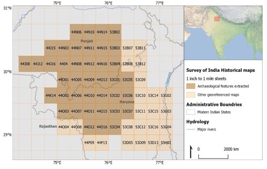
Figure 7.
Geographical location of the georeferenced Survey of India 1” to 1-mile map sheets used in this study.
5. Identifying mound features on Survey of India 1” to 1-mile maps
With the maps georectified, it is possible to extract features of archaeological interest with a high degree of accuracy, and the manual detection and digitisation was carried out by several of the co-authors. Two GIS shapefiles were created to store the results of the digitisation, one for points and another for linear features. Both shapefiles had an associated table with columns destined to store information about the digitised features. These information categories included location coordinates, feature type, relief height and size, which were chosen to offer the maximum possible detail about the original features to assist future analysis (see below).
The point layer shapefile was dedicated to the digitisation of mound features depicted in the maps and recorded a single point per mound located in the geometrical centre of the feature. The table associated with this layer included information about the individual maps, edition, and year of publication of the map from which each point was retrieved, but also important data about each individual feature that was recorded. The type and colour of the line used to represent the mound features was noted as it provides an important indication of how the surveyor perceived the feature while in the field. As noted above, the methods used by the Survey of India meant that features and/or mounds that were similar in terms of size, shape and height might have been drawn using different methods, including ‘horizontal’ continuous contour lines, discontinuous ‘form-lines’, shaded relief, ‘vertical’ hatching or using a combination of these approaches (see below).
The size of the mounds was measured using the largest axis of the feature, and we opted to divide them into three categories: (1) mound features measuring up to 200 m, which were the most common and typically measure around 100 m; (2) mound features between 200 and 400 m, and (3) mound features with diameters of more than 400 m. As many of the Survey of India 1” to 1-mile maps provide information on the relative height of the mound features in feet, it was also often possible to include a measure of height, which in combination with the measure of sizes provides a useful way to characterise the volume and character of each mound feature. Spot heights on these mounds were taken during the process of surveying, and the elevation of the mounds may have made them suitable places for circuit stations or survey points.
The second shapefile layer aimed at recording linear features. These appear to consist mostly of earthworks and relict field systems, and lines were recorded following the axis of the features. Apart from the information relative to the map from which linear features were extracted, the table associated to the linear feature shapefile layer included information on the type of line and relative height of the feature. The tables for both layers also included a field in which notes about the digitisation process could be included.
Digitisation was carried out using both ArcMap and QGIS. The manual digitisation of map features followed a systematic grid to ensure no areas were left uninspected. Observation of individual sheets and sets of sheets showed that mounds could be represented using three main approaches:
(a) ‘shaded mound features’, which were delineated with graded stippling and are perhaps the most common way of representing mounds, particularly those in the small size (1) category (Figure 8a). According to the Survey of India 1” to 1-mile map legends, these features were defined as ‘sand-hills’, and the darker shading around the edges and/or a spot height indicates that they were formally surveyed (Figure 8a);
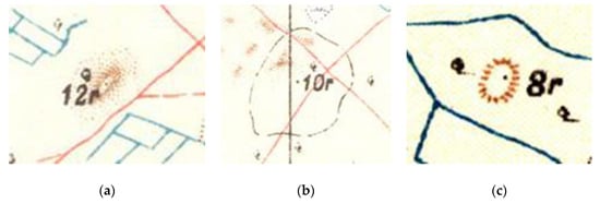
Figure 8.
(a) Shaded; (b) Form-line; (c) Hachure mound features (Images courtesy of Cambridge University Library).
(b) ‘form-line mound features’, which were delineated using a discontinuous horizontal brown or black line (Figure 8b) that was usually employed for medium size (2) and large size (3) mounds. The use of discontinuous ‘form-lines’ indicates that they represent clear areas of elevation. The use of the horizontal rather than vertical lines to depict elevation is potentially related to the shallowness of the slope. It is likely that the form-lines were used as break-lines marking the transition between the flat plain and the elevated mound. The presence of a spot height presumably marks the highest point of the mound. In the process of hill-sketching, Surveyors were advised to use 25 feet contours ([9], p. 557), so an elevation of up to 7.5 m would have only warranted one contour. The choice to use form lines rather than contours to depict such mounds is interesting, as it suggests that they were recognised as not being natural hills, but there are no clear references to methods for depicting such features in either edition of A Manual of Surveying for India [9,65];
(c) ‘hachure mound features’ were delineated using vertical lines to depict elevation, which was potentially related to the steepness of the slope. Vertical hachures were sometimes used to represent small (1) and medium size (2) mounds (Figure 8c).
Figure 9 shows the range of mound feature types that can appear on one sheet. This includes instances where a combination of approaches was employed to represent a mound feature, and in these cases, we used a ‘combined’ category.
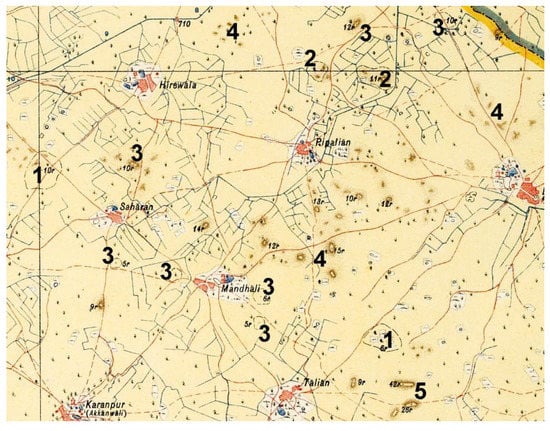
Figure 9.
Survey of India 1” to 1-mile map sheet of 44/O5/1915. Large mounds delineated by form-lines are labelled 1, and ‘combined’ features showing both form-lines and shaded relief are labelled 2. Medium-sized mounds delineated by either shading or form-lines are labelled 3, while clusters of small mound features delineated with shading are labelled 4. Linear mound features that may be traces of elevated roads or sand dunes are labelled 5 (Base map image courtesy of Cambridge University Library).
The use of continuous black lines to demarcate small features can be confusing, but it appears that these typically represent ponds (Figure 10a,b). When ponds contained water they were coloured blue (Figure 10a), while those that were dry at the time of survey were represented as a continuous black line without a colour fill (Figure 10b). Lines formed of points also appear, and appear to represent areas under cultivation (Figure 10c, also Figure 10a).
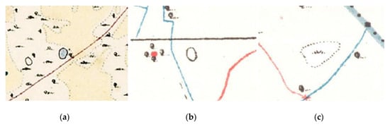
Figure 10.
(a) Full pond; (b) Dry pond; (c) Dotted line feature (Images courtesy of Cambridge University Library).
Figure 11a,b show the types of relationships that existed between some linear and mound features. Mound features are visible to the top left of Figure 11a [(b) form-line] and towards the centre of Figure 11b [(c) hachure marked with a relative height of 8 feet]. It is evident that some the lineal mound features follow the orientation and direction of then-modern roads, suggesting that they potentially follow earlier routes. Figure 11b also shows how water channels go around mound features, potentially because of the topography created by the mound, which needed to be avoided for the water to flow. Figure 11c shows a combined mound feature, where a discontinuous form-line co-occurs with graves. In these instances, it is likely that the graves were relatively modern, and were excavated into an existing mound feature.
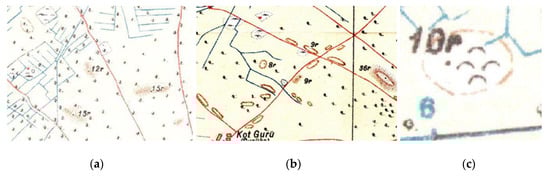
Figure 11.
(a) Form-line and linear shaded mound features with spot heights on the same sheet; (b) Hachure and linear shaded mound features with spot heights and close to roads on the same sheet; (c) Combination of mound and graves (Images courtesy of Cambridge University Library).
Almost 9000 mound features (Table 2) have been identified on 40 of the 64 Survey of India 1” to 1-mile map sheets listed in Table 1 (Figure 7). Within the area investigated for this study, shaded, form-line and hachure features were all common, but there is considerable variability in the number and size categories of mounds attested on individual sheets. The size 1 features in each category were the most abundant, but proportionally significant numbers of size 2 and 3 features were also located.
Table 2.
The mound feature type and size categories of features recorded on the georeferenced maps.
The variability in mound feature occurrence indicates that it is not yet statistically robust to attempt to produce summative data on the average number of mound features and the frequency of specific types per sheet, or to consider extrapolating this across a larger area. In future, when sheets that cover the full range of climate and ecological zones have been assessed, it will be possible to carry out predictive modelling of the number of mound types and size categories that might be expected in different zones.
6. Testing the Archaeological Viability of the Identification of Mound Features
The viability of the categorisation outlined here has been tested in the field over several field seasons [84,85,86,87] (Figure 12), and the detailed results of this analysis are the subject of a separate paper [88]. To facilitate the process of ground-truthing, each feature location was included in a field survey table and assigned Historical Feature Identification Numbers (hf_id), which will be used to create a comprehensive listing of preserved and potentially lost archaeological sites. Each hf_id was accompanied by information about its feature type and size category to allow the field survey team to assess the probability that a feature identified on the historical maps remains identifiable in the contemporary landscape, and the probability that the hf_id is (or more correctly, was) an archaeological site.
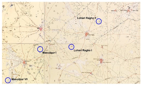
Figure 12.
Four map sheets combined to show the area to the southwest of the Indus Civilisation urban site of Rakhigarhi (visible as a number of mounds under two modern villages at top right; also Figure 6), and the location of a selection of form-line mound features that correspond with surveyed archaeological sites (Base map image courtesy of Cambridge University Library).
A sample of mound features in the size (2) or size (3) (i.e., those greater than 200 m across on the 1” to 1-mile maps) categories were visited and assessed to determine whether they were extant archaeological sites. This resulted in the identification of in excess of 200 archaeological sites within a delimited study area that were previously unknown [86,87,88]. In the early stages of this survey, it became clear that the smallest features on the historical maps were rarely preserved. As a result, in each survey unit, historical mound features in the size (1) category were visited until at least ten features tested negative. In many instances, this meant that every historical mound feature identified in a survey unit was visited, but in some, several size (1) historical mound features were not visited as their likelihood of being a preserved archaeological site was demonstrably low. It is clear that it is not feasible to simply assume that all mound features were archaeological sites, not least because there is variation in the detail and clarity of each feature, and some of these features are almost certainly geomorphological in origin. Importantly, there is significant variation in the number of mound features on each map, as some have 400+ features, while others have as few as 60. This variability by sheet no doubt reflects variation on the ground, with some areas having more features, and potentially more sites. In addition to checking mound features, it is also possible to visit locations that include topographic words within the name to ascertain whether archaeological mounds are present. It has been noted previously that a number of modern villages in this region are elevated, and are likely built on top of archaeological sites. Ground-truthing is the essential component for demonstrating the veracity of the historic map dataset. It is also important to remember that many sites have been lost as agricultural development in the region has unfolded, which is a factor that will need to be considered in future studies.
7. Discussion and Conclusions
Imperial mapping projects in South Asia were inevitably geared towards the systematic documentation of the landscape to facilitate military domination, administrative control and economic exploitation. The Survey of India and the Archaeological Survey of India began as large-scale systematic documentation projects, and there are clear instances where information about archaeological sites that had been documented made its way onto 1” to 1-mile maps (e.g., Figure 5). There are, however, also numerous instances where otherwise undocumented archaeological sites were recorded on these maps (e.g., Figure 6 and Figure 12), but the historical significance of these mound features does not appear to have been recognised formally at the time. It appears unlikely that the surveying teams were aware of the archaeological significance of what they were recording by and large, but the appearance of village names with some appellation of mound incorporated suggests that there was some awareness amongst local populations that these mounds were something unusual. Furthermore, many of these mounds are likely to have had significance for local populations as they were areas of sacred spaces as cemeteries, areas of economic exploitation – most particularly silt, sand and brick extraction - and their elevation means that they were not well suited for irrigation supported agriculture. This last factor also means that many mounds are currently under threat due to pressure from extensive and intensive farming and the ready availability of bulldozers.
These maps provide a new resource that can now be used to take major steps towards understanding long-term trajectories of human occupation in South Asia, and they will make it possible to develop new inclusive, comprehensive, and decolonised records of these evolving social landscapes. The systematic documentation of mound features visible on historic maps will make it possible to filter and query the data set at a later stage to select specific types of features, create thematic maps, quantify aspects of those features, and perform statistical analyses. Although substantial numbers of archaeological sites have already been documented across northwest India [75,76,77,78], attempts to conduct systematic survey using historic maps as a key data source has shown that the currently ‘known’ sites represent only a fraction of the actual archaeological settlements in the region [84,85,86,87,88]. Although a large number of the almost 9000 mound features visible in the historical maps that have been studied are likely to be natural, if even one tenth of them turn out to be archaeological sites, then the number of known sites in the region will increase dramatically. The Survey of India 1” to 1-mile maps thus have the potential to revolutionise our understanding of the archaeological landscapes of South Asia.
Beyond their use for identifying and locating hitherto unrecognised archaeological mound sites, these 1” to 1-mile maps have considerable potential for reconstructing other types of landscape features that are also often overlooked, including palaeochannel levees, relict sand-dunes, raised road-ways and relict field-systems [89]. This historical map data set can also be used to reconstruct historical landscape dynamics [90], and/or the development of land-use practices, hydrological schemes and irrigation, and urban growth from the late nineteenth and early twentieth centuries.
As with other remote sensing and aerial photography datasets, there are inevitably a range of limitations to the Survey of India 1” to 1-mile maps, not least the fact that some areas were mapped repeatedly, while others do not appear to have ever had maps produced and/or made publically available. There are, however, extant archives that contain maps of areas of archaeological interest, and further research will require the establishment of new collaborations involving scholars and governmental institutions in Pakistan, India and Afghanistan. The 1” to 2-mile and 1” to 4-mile maps typically cover the interstitial areas, and they also document important archaeological data, but these series are inevitably of lower resolution. Nonetheless, they are an additional data source that also needs to be considered.
It is important to acknowledge that the methods outlined here for making use of these Survey of India 1” to 1-mile maps are only likely to be useful for identifying mounded sites, and will not be suitable to aid detection of a wide range of other features of archaeological significance. Therefore, it is essential to integrate the use of these historical maps into comprehensive approaches that make use of the full suite of earth observation and remote sensing techniques, potentially integrating open-source multi-spectral data and the computational power of platforms like Google Earth Engine to identify hydrological and topographic features not easily visible on the surface [35,90,91]. It is also imperative that these remote prospection approaches are co-ordinated with large-scale ground-truthing surveys, that will verify which of the mound features are archaeological sites, and establish a reliable chronology for those sites and the associated landscapes. The combined analysis of these maps and the ground-truthing of the mound feature data will also make it possible to use machine learning-based approaches to carry out site detection across very large areas.
It is particularly timely to be able to add new evidence for the distribution of old settlements. The sobering truth is that in many instances, mound features in South Asia that were recorded in the early twentieth century are no longer extant, and in areas where farming is becoming increasingly mechanised and urban growth is unabated, mounds are disappearing with increasing speed. When such circumstances are in play archaeological sites and cultural heritage are clearly at-risk, and large-scale integrated mapping and survey projects cannot be commenced soon enough.
Author Contributions
Conceptualization, C.A.P., J.R.K. and R.N.S.; formal analysis, H.A.O., A.S.G., J.R.W., A.G. and F.C.; method, H.A.O.; writing—original draft, C.A.P. and H.A.O.; writing—review and editing, C.A.P., H.A.O., A.S.G., J.R.W., A.G., F.C., J.R.K. and R.N.S.
Funding
The Land, Water and Settlement project was primarily funded by a Standard Award from the UK India Education and Research Initiative (UKIERI) under the title “From the collapse of Harappan urbanism to the rise of the great Early Historic cities: investigating the cultural and geographical transformation of northwest India between 2000 and 300 B.C.”. Smaller grants were also awarded by the British Academy’s Stein Arnold Fund, the Isaac Newton Trust, the McDonald Institute for Archaeological Research and the Natural Environment Research Council (NERC). The TwoRains project has been primarily funded by the European Research Council under the European Union’s Horizon 2020 research and innovation program (grant agreement no. 648609), but has also received support from DST/UKIERI, the British Academy and the McDonald Institute for Archaeological Research. The WaMStrIn and Marginscapes projects have been funded by the European Union’s Horizon 2020 Research and Innovation programme under the Marie Skłodowska-Curie grant agreement no.s 746446 and 794711.
Acknowledgments
The research presented in this paper is the product of the long-term consideration of the importance of historic maps for understanding archaeological landscapes. Following initial steps made by J.R. Knox, the Land, Water and Settlement project made extensive use of these historic maps during reconnaissance and more extensive surveys, and the TwoRains project has developed a comprehensive method for using these maps as a large-scale data source for archaeological landscape reconstruction. The work of TwoRains has also been enhanced by two related projects entitled WaMStrIn and Marginscapes. The authors would like to thank the heads of the Department of AIHC and Archaeology at Banaras Hindu University and the Department of Archaeology at the University of Cambridge who have provided their support to the Land, Water and Settlement, TwoRains, WaMStrIn and Marginscapes projects. We would especially like to thank the staff of the Map Room and Imaging Services at the University Library at the University of Cambridge for providing access to and high-resolution copies of the Survey of India 1” to 1-mile maps in their collection.
Conflicts of Interest
The authors declare no conflict of interest.
References
- Wilkinson, T.J. Archaeological Landscapes of the Near East; University of Arizona Press: Tucson, AZ, USA, 2003. [Google Scholar]
- Petrie, C.A. Remote sensing in inaccessible lands: Plains and preservation along old routes between Pakistan and Afghanistan. ArchAtlas 2007, 3. Available online: http://www.archatlas.org/workshop/Petrie07.php (accessed on 8 November 2018).
- Thomas, D.C.; Kidd, F.J. On the margins: Enduring pre-modern water management strategies in and around the Registan desert, Afghanistan. J. Field Archaeol. 2017, 41, 29–42. [Google Scholar] [CrossRef]
- Hammer, E.; Seifried, R.; Franklin, K.; Lauricellaca, A. Remote assessments of the archaeological heritage situation in Afghanistan. J. Cult. Herit. 2018, 33, 125–144. [Google Scholar] [CrossRef]
- Franklin, K.; Hammer, E. Untangling palimpsest landscapes in conflict zones: A “remote survey” in Spin Boldak, Southeast Afghanistan. J. Field Archaeol. 2018, 43, 58–73. [Google Scholar] [CrossRef]
- Casana, J.; Laugier, E.J. Satellite imagery-based monitoring of archaeological site damage in the Syrian civil war. PLoS ONE 2017, 12, e0188589. [Google Scholar] [CrossRef] [PubMed]
- Orengo, H.A.; Krahtopoulou, A.; Garcia-Molsosa, A.; Palaiochoritis, K.; Stamati, A. Photogrammetric re-discovery of the hidden long-term landscapes of western Thessaly, central Greece. J. Archaeol. Sci. 2015, 64, 100–109. [Google Scholar] [CrossRef]
- Simpson, T. “Clean out of the map”: Knowing and doubting space at India’s high imperial frontiers. Hist. Sci. 2017, 55, 3–36. [Google Scholar] [CrossRef]
- Thuillier, H.L.; Smyth, R. A Manual for Surveying for India Detailing the Mode of Operations on the Trigonometrical, Topographical and Revenue Surveys of India, 3rd ed.; Thacker, Spink and Co.: Calcutta, India, 1875. [Google Scholar]
- Fairservis, W.A. Excavations in the Quetta Valley, West Pakistan; American Museum of Natural History: New York, NY, USA, 1956. [Google Scholar]
- Wiseman, J.R.; El-Baz, F. (Eds.) Remote Sensing in Archaeology; Springer: New York, NY, USA, 2007. [Google Scholar]
- Tapete, D. Remote Sensing and Geosciences for Archaeology. Geosciences 2018, 8, 41. [Google Scholar] [CrossRef]
- Fowler, M.J.F.; Curtis, H. Stonehenge from 230 kilometres. AARGnews 1995, 11, 8–16. [Google Scholar]
- Kennedy, D. Declassified satellite photographs and archaeology in the Middle East: Case studies from Turkey. Antiquity 1998, 72, 553–561. [Google Scholar] [CrossRef]
- Kouchoukos, N. Satellite images and the representation of Near Eastern landscapes. Near East. Archaeol. 2001, 64, 80–91. [Google Scholar] [CrossRef]
- Ogata, N. A study on cities, settlements and archaeological sites in the Silk Road region using satellite photos. Bull. Res. Cent. Silk Roadol. 2003, 17, 39–51. Available online: http://hdl.handle.net/10935/4395 (accessed on 9 November 2018).
- Pournelle, J. Marshland of Cities: Deltaic Landscapes and the Evolution of Early Mesopotamian Civilization. Ph.D. Dissertation, University of California, San Diego, CA, USA, 2003. [Google Scholar]
- Ur, J.A. CORONA satellite photography and ancient road networks: A northern Mesopotamian case study. Antiquity 2003, 77, 102–115. [Google Scholar] [CrossRef]
- Fowler, M.J.F. Declassified CORONA KH-4B satellite photography of remains from Rome’s desert frontier. Int. J. Remote Sens. 2004, 25, 3549–3554. [Google Scholar] [CrossRef]
- Galiatsatos, N. Assessment of the CORONA series of satellite imagery for landscape archaeology: A case study from the Orontes valley, Syria. Unpublished. Ph.D. Dissertation, Durham University, Durham, UK, 2004. [Google Scholar]
- Wilkinson, T.J.; Ur, J.; Casana, J. From nucleation to dispersal: Trends in settlement pattern in the Northern Fertile Crescent. In Side-by-Side Survey: Comparative Regional Studies in the Mediterranean World; Cherry, J., Alcock, S., Eds.; Oxbow Books: Oxford, UK, 2004; pp. 198–205. ISBN 1842170961. [Google Scholar]
- Altaweel, M. The use of ASTER satellite imagery in archaeological contexts. Archaeol. Prospect. 2005, 166, 151–166. [Google Scholar] [CrossRef]
- Hritz, C. The changing archaeoscape of southern Mesopotamia. In GIS and Archaeological Site Location Modelling; Mehrer, M., Wolcott, C., Eds.; Taylor & Francis: Boca Raton, FL, USA, 2005; pp. 413–436. ISBN 9780415315487. [Google Scholar]
- Alizadeh, K.; Ur, J.A. Formation and destruction of pastoral and irrigation landscapes on the Mughan Steppe, north-western Iran. Antiquity 2007, 81, 148–160. [Google Scholar] [CrossRef]
- Beck, A.; Philip, G.; Abdulkarim, M.; Donoghue, D.N. Evaluation of Corona and Ikonos high resolution satellite imagery for archaeological prospection in western Syria. Antiquity 2007, 81, 161–175. [Google Scholar] [CrossRef]
- Casana, J.; Cothren, J. Stereo analysis, DEM extraction and orthorectification of CORONA satellite imagery: Archaeological applications from the Near East. Antiquity 2008, 82, 732–749. [Google Scholar] [CrossRef]
- Mantellini, S.; Rondelli, B.; Stride, S. Analytical approach for representing the water landscape evolution in Samarkand Oasis (Uzbekistan). In On the Road to Reconstructing the Past. Computer Applications and Quantitative Methods in Archaeology (CAA2008); Jerem, E., Redö, F., Szeverényi, V., Eds.; Archaeolingua: Budapest, Hungary, 2011; pp. 387–396. ISBN 9789639911307. [Google Scholar]
- Rondelli, B.; Stride, S.; García-Granero, J.J. Soviet military maps and archaeological survey in the Samarkand region. J. Cult. Herit. 2013, 14, 270–276. [Google Scholar] [CrossRef]
- Ur, J.; de Jong, L.; Giraud, J.; Osborne, J.F.; MacGinnis, J. Ancient cities and landscapes in the Kurdistan region of Iraq: The Erbil Plain Archaeological Survey 2012 season. Iraq 2013, 75, 89–118. [Google Scholar] [CrossRef]
- Wright, R.P.; Hritz, C. Satellite remote sensing imagery: New evidence for site distributions and ecologies in the upper Indus. In South Asian Archaeology 2007; Frenez, D., Tosi, M., Eds.; BAR International Series 2454; Archaeopress: Oxford, UK, 2013; pp. 315–321. ISBN 9781407310626. [Google Scholar]
- Conesa, F.C.; Madella, M.; Galiatsatos, N.; Balbo, A.L.; Rajesh, S.V.; Ajithprasad, P. CORONA photographs in monsoonal semi-arid environments: Addressing archaeological surveys and historic landscape dynamics over North Gujarat, India. Archaeol. Prospect. 2015, 22, 75–90. [Google Scholar] [CrossRef]
- Ogata, N.; Yu, Z.; Ito, T.; Sohma, H.; Ideta, K. A study of settlement remains near the Qiemo Oasis in Northwestern China using Satellite Imagery and DEM. Stud. Geogr. Reg. Environ. Res. 2015, VIII, 9–29. Available online: http://jairo.nii.ac.jp/0059/00005522 (accessed on 9 November 2018).
- Hammer, E. New Research Directions in the CAMEL Lab. News and Notes, The Oriental Institute Members’ Magazine. 2016, Volume 228, pp. 4–9. Available online: https://oi.uchicago.edu/sites/oi.uchicago.edu/files/uploads/shared/docs/Publications/nn228-web.pdf (accessed on 9 November 2018).
- Hammer, E.; Lauricella, A. Historical imagery of desert kites in eastern Jordan. Near East. Archaeol. 2017, 80, 74–83. [Google Scholar] [CrossRef]
- Orengo, H.A.; Petrie, C.A. Large-scale, multi-temporal remote sensing of palaeo-river networks: A case-study from northwest India and its implications for the Indus Civilisation. Remote Sens. 2017, 9, 735. [Google Scholar] [CrossRef]
- Thomas, D.C. The Ebb and Flow of the Ghūrid Empire; Adapa Monographs; University of Sydney Press: Sydney, Australia, 2018; ISBN 9781743325414. [Google Scholar]
- Fuentes, J.; Varga, D.; Pinto, J. The Use of High-Resolution Historical Images to Analyse the Leopard Pattern in the Arid Area of La Alta Guajira, Colombia. Geosciences 2018, 8, 366. [Google Scholar] [CrossRef]
- Scollar, I.; Galiatsatos, N.; Mugnier, C. Mapping from CORONA geometric distortion in KH4 images. Photogramm. Eng. Remote Sens. 2016, 82, 7–13. [Google Scholar] [CrossRef]
- Crawford, O.G.S. A century of air photography. Antiquity 1954, 28, 206–210. [Google Scholar] [CrossRef]
- Kennedy, D.; Bewley, R. Aerial archaeology in Jordan. Antiquity 2009, 83, 69–81. [Google Scholar] [CrossRef]
- Braasch, O. Goodbye Cold War! Goodbye Bureaucracy? Opening the skies to aerial archaeology. In Aerial Archaeology: Developing Future Practice; Bewley, R., Rączkowski, W., Eds.; IOS Press: Amsterdam, The Netherlands, 2002; pp. 19–22. ISBN 1586031848. [Google Scholar]
- Bourgeois, J.; Meganck, M. (Eds.) Aerial Photography and Archaeology 2003: A Century of Information; Archaeological Reports Ghent University; Academia: Ghent, Belgium, 2005; ISBN 9789038207827. [Google Scholar]
- Hanson, W.S.; Oltean, I.A. (Eds.) Archaeology from Historical Aerial and Satellite Archives; Springer: New York, NY, USA, 2013; ISBN 978-1-4614-4505-0. [Google Scholar]
- Orengo, H.A.; Knappett, C. Toward a definition of Minoan agro-pastoral landscapes: Results of the survey of Palaikastro (Crete). Am. J. Archaeol. 2018, 122, 470–507. [Google Scholar] [CrossRef]
- Grady, D. Aerial Reconnaissance: Management of Research Projects in the Historic Environment; MoRPHE Project Planning Notes (PPN) 5; Historic England: London, UK, 2008; Available online: https://historicengland.org.uk/images-books/publications/morphe-project-planning-note-5/heag028-morphe-ppn5/ (accessed on 9 November 2018).
- Verhoeven, G.; Sevara, C.; Karel, W.; Ressl, C.; Doneus, M.; Briese, C. Undistorting the past: New techniques for orthorectification of archaeological aerial frame imagery. In Good Practice in Archaeological Diagnostics: Non-Invasive Survey of Complex Archaeological Sites; Corsi, C., Slapšak, B., Vermeulen, F., Eds.; Natural Science in Archaeology; Springer: Cham, Switzerland, 2013; pp. 31–67. ISBN 978-3-319-01784-6. [Google Scholar]
- Doneus, M.; Geert Verhoeven, G.; Atzberger, C.; Wess, M.; Ruš, M. New ways to extract archaeological information from hyperspectral pixels. J. Archaeol.l Sci. 2014, 52, 84–96. [Google Scholar] [CrossRef]
- McCarthy, J. Multi-image photogrammetry as a practical tool for cultural heritage survey and community engagement. J. Archaeol. Sci. 2014, 43, 175–185. [Google Scholar] [CrossRef]
- Oliver, R. Ordnance Survey Maps: A Concise Guide for Historians; Charles Close Society for the Study of Ordnance Survey Maps: London, UK, 2005; ISBN 978-1-870-598-31-6. [Google Scholar]
- Phillips, C.W. Archaeology in the Ordnance Survey 1791–1965; CBA: London, UK, 1980; ISBN 0900312904. [Google Scholar]
- Edney, M.H. Mapping an Empire: The Geographical Construction of British India, 1765–1843; University of Chicago Press: Chicago, IL, USA, 1997; ISBN 9780226184883. [Google Scholar]
- Barrow, I.J. Making History, Drawing Territory: British Mapping in India, c.1756–1905; Oxford University Press: Oxford, UK, 2003; ISBN 0195665465. [Google Scholar]
- Chester, L.P. Borders and Conflict in South Asia: The Radcliffe Boundary Commission and the Partition of Punjab; Studies in Imperialism; Manchester University Press: Manchester, UK, 2009; ISBN 978-0-7190-9136-0. [Google Scholar]
- Foliard, D. Dislocating the Orient: British Maps and the Making of the Middle East, 1854–1921; University of Chicago Press: Chicago, IL, USA, 2017; ISBN 9780226451336. [Google Scholar]
- Ball, W. Archaeological Gazetteer of Afghanistan/Catalogue des Sites Archéologiques d’Afghanistan; Editions Recherche sur les Civilisations: Paris, France, 1982; ISBN 2-86538-040-8. [Google Scholar]
- Hewitt, R. Map of a Nation—A Biography of the Ordnance Survey; Granta: London, UK, 2010; ISBN 978-1847082541. [Google Scholar]
- Chadha, S.M. Survey of India through the Ages; Royal Institution of Chartered Surveyors and the Royal Geographical Society: London, UK, 1990. [Google Scholar]
- Chadha, S.M. Survey of India through the ages. Himal. J. 1991, 47. Available online: https://www.himalayanclub.org/hj/47/2/survey-of-india-through-the-ages/ (accessed on 9 November 2018).
- Roy, W. An account of the mode proposed to be followed in determining the relative situation of the Royal Observatories of Greenwich and Paris. Philos. Trans. R. Soc. Lond. 1787, 77, 188–226. [Google Scholar] [CrossRef]
- Scholberg, H. The District Gazetteers of British India: A Bibliography; Inter Documentation: Zug, Switzerland, 1970; ISBN 9780800212650. [Google Scholar]
- Hunter, W.W. The Imperial Gazetteer of India; Clarendon Press: Oxford, UK, 1881. [Google Scholar]
- Black, C.E.D. A Memoir on the Indian Surveys, 1875–1890; E.A. Arnold: London, UK, 1891. [Google Scholar]
- Phillimore, R.H. Historical Records of the Survey of India; Survey of India: Dehra Dun, India, 1945–1968; Volumes 1–5. [Google Scholar]
- Kulkarni, M.N. Two centuries of surveying and mapping in India. Surv. Rev. 2006, 38, 452–458. [Google Scholar] [CrossRef]
- Smyth, R.; Thuillier, H.L. A Manual for Surveying for India Detailing the Mode of Operations on the Trigonometrical, Topographical and Revenue Surveys of India, 1st ed.; Thacker and Co.: Calcutta, India, 1851. [Google Scholar]
- Public Website. Available online: https://pahar.in/survey-of-india-report-maps/ (accessed on 8 November 2018).
- Cunningham, A. Four Reports Made During the Years 1862-673-64-65; Archaeological Survey of India Reports; Archaeological Survey of India: Calcutta, India, 1871; Volume I. [Google Scholar]
- Cunningham, A. The Ancient Geography of India; Chuckervertty, Chatterjee and Co.: Calcutta, India, 1871. [Google Scholar]
- Murray, D. Ordnance survey and the depiction of antiquities on maps: Past, present and future: The current and future role of the Royal Commissions as suppliers of heritage data to the Ordnance Survey. In Archaeology in the Age of the Internet. CAA97. Computer Applications and Quantitative Methods in Archaeology; Dingwall, L., Exon, S., Gaffney, V., Laflin, S., van Leusen, M., Eds.; BAR International Series 750; Archaeopress: Oxford, UK, 1999; pp. 235–239. ISBN 0860549453. [Google Scholar]
- Seymour, W.A. A History of the Ordnance Survey; Dawson: Folkestone, UK, 1980; ISBN 9780712909792. [Google Scholar]
- Godwin-Austin, A. The Conference of Empire Surveyors. Geogr. J. 1928, 72, 449–453. Available online: https://www.jstor.org/stable/1783349 (accessed on 9 November 2018).
- Evans, C.J.; Brittain, M.; Cessford, C. Inlands and Hinterlands: The Archaeology of North West Cambridge; CAU New Archaeologies of the Cambridge Region Series; McDonald Institute: Cambridge, UK; Volume IV, in preparation.
- Crawford, O.G.S. Primitive English land-marks and maps. Emp. Surv. Rev. 1931, 1, 3–12. [Google Scholar]
- Survey Review. Empire Conference of Survey Officers 1928. Surv. Rev. 2006, 38, 434–435. [Google Scholar] [CrossRef]
- Joshi, J.P.; Bala, M.; Ram, J. The Indus Civilisation: A reconsideration on the basis of distribution maps. In Frontiers of the Indus Civilisation: Sir Mortimer Wheeler Commemoration Volume; Lal, B.B., Gupta, S.P., Eds.; Books & Books: Delhi, India, 1984; pp. 511–530. ISBN 9780856722318. [Google Scholar]
- Possehl, G.L. Indus Age: The Beginnings; U Penn Museum: Philadelphia, PA, USA, 1999; ISBN 978-0812234176. [Google Scholar]
- Kumar, M. Harappan settlements in the Ghaggar-Yamuna divide. In Linguistics. Archaeology and the Human Past; Indus Project, Research Institute for Humanity and Nature: Kyoto, Japan, 2009; Volume 7, pp. 1–75. ISBN 9784902325423. [Google Scholar]
- Green, A.S.; Petrie, C.A. Landscapes of urbanisation and de-urbanization: Integrating site location datasets from northwest India to investigate changes in the Indus Civilization’s settlement distribution. J. Field Archaeol. 2018, 43, 284–299. [Google Scholar] [CrossRef]
- Possehl, G.L. A short history of archaeological discovery at Harappa. In Harappa Excavations 1986–1990: A Multi-Disciplinary Approach to Third Millennium Urbanism; Meadow, R.H., Ed.; Monographs in World Archaeology No. 3; Prehistory Press: Madison, WI, USA, 1996; pp. 5–11. ISBN 9780962911019. [Google Scholar]
- Cunningham, A. Report for the Year 1872–73; Archaeological Survey of India Reports; Archaeological Survey of India: Calcutta, India, 1875; Volume V. [Google Scholar]
- Gazetteer of Attock District 1930; Punjab District Gazetteers: Lahore, Pakistan, 1932.
- ArcGIS Desktop, Fundamentals of Georeferencing A Raster Dataset. Available online: http://desktop.arcgis.com/en/arcmap/latest/manage-data/raster-and-images/fundamentals-for-georeferencing-a-raster-dataset.htm (accessed on 9 November 2018).
- Petrie, C.A.; Singh, R.N.; Bates, J.; Dixit, Y.; French, C.A.I.; Hodell, D.; Jones, P.J.; Lancelotti, C.; Lynam, F.; Neogi, S.; et al. Adaptation to variable environments, resilience to climate change: Investigating Land, Water and Settlement in northwest India. Curr. Anthropol. 2017, 58, 1–30. Available online: http://www.journals.uchicago.edu/doi/full/10.1086/690112 (accessed on 9 November 2018). [CrossRef]
- Singh, R.N.; Petrie, C.A.; Pawar, V.; Pandey, A.K.; Neogi, S.; Singh, M.; Singh, A.K.; Parikh, D.; Lancelotti, C. Changing patterns of settlement in the rise and fall of Harappan urbanism: Preliminary report on the Rakhigarhi Hinterland Survey 2009. Man Environ. 2010, 35, 37–53. [Google Scholar]
- Singh, R.N.; Petrie, C.A.; Pawar, V.; Pandey, A.K.; Parikh, D. New insights into settlement along the Ghaggar and its hinterland: A preliminary report on the Ghaggar Hinterland Survey 2010. Man Environ. 2011, 36, 89–106. [Google Scholar]
- Singh, R.N.; Green, A.S.; Green, L.M.; Ranjan, A.; Alam, A.; Petrie, C.A. Between the Hinterlands: Preliminary Results from the TwoRains Survey in Northwest India 2017. Man Environ. 2018, in press. [Google Scholar]
- Singh, R.N.; Green, A.S.; Alam, A.; Petrie, C.A. Beyond the Hinterlands: Preliminary Results from the TwoRains Survey in Northwest India 2018. Man Environ. 2019, in press. [Google Scholar]
- Green, A.S.; Singh, R.N.; Alam, A.; Garcia, A.; Green, L.M.; Conesa, F.; Orengo, H.A.; Ranjan, A.; Petrie, C.A. Re-discovering dynamic ancient landscapes: Archaeological survey of features from historical maps in northwest India and their implications for the large-scale distribution of settlements throughout South Asia. Remote Sens. in preparation.
- Walker, J.R. Human-Environment Interactions in the Indus Civilisation: Reassessing the Role of Rivers, Rain and Climate Change in northwest India. Ph.D. Thesis, Department of Archaeology, University of Cambridge, Cambridge, UK. in preparation.
- Garcia, A.; Orengo, H.A.; Conesa, F.C.; Green, A.S.; Petrie, C.A. Remote Sensing and historical morphodynamics of alluvial plains: The 1909 Indus flood and the city of Dera Ghazi Khan (Province of Punjab, Pakistan). Geosciences 2018, 9, in press. [Google Scholar]
- Orengo, H.A.; Petrie, C.A. Multi-Scale Relief Model (MSRM): A new algorithm for the analysis of subtle topographic change in digital elevation models. Earth Surf. Process. Landf. 2018, 43, 1361–1369. [Google Scholar] [CrossRef] [PubMed]
© 2018 by the authors. Licensee MDPI, Basel, Switzerland. This article is an open access article distributed under the terms and conditions of the Creative Commons Attribution (CC BY) license (http://creativecommons.org/licenses/by/4.0/).