Numerical Modelling of Salt-Related Stress Decoupling in Sedimentary Basins–Motivated by Observational Data from the North German Basin


Institute of Applied Geosciences, TU Darmstadt, Schnittspahnstraße 9, 64287 Darmstadt, Germany
*
Author to whom correspondence should be addressed.
Geosciences 2019, 9(1), 19; https://doi.org/10.3390/geosciences9010019
Submission received: 12 October 2018
/
Revised: 17 December 2018
/
Accepted: 19 December 2018
/
Published: 29 December 2018
(This article belongs to the Special Issue Stress Quantification in Sedimentary Basins)
Abstract
:A three dimensional (3D) finite element model is used to study the conditions leading to mechanical decoupling at a salt layer and vertically varying stress fields in salt-bearing sedimentary basins. The study was inspired by observational data from northern Germany showing stress orientations varying up to 90° between the subsalt and the suprasalt layers. Parameter studies address the role of salt viscosity and salt topology on how the plate boundary forces acting at the basement level affect the stresses in the sedimentary cover above the salt layer. Modelling results indicate that mechanical decoupling occurs for dynamic salt viscosities lower than 1021 Pa·s, albeit this value depends on the assumed model parameters. In this case, two independent stress fields coexist above and below the salt layer, differing in tectonic stress regime and/or stress orientation. Thereby, stresses in the subsalt domain are dominated by the shortening applied, whereas in the suprasalt section they are controlled by the local salt topology. For a salt diapir, the orientation of the maximum horizontal stress changes from a circular pattern above to a radial pattern adjacent to the diapir. The study shows the value of geomechanical models for stress prediction in salt-bearing sedimentary basins providing a continuum mechanics–based explanation for the variable stress orientations observed.

1. Introduction
Lateral variations in the orientation of the maximum horizontal stress (SHmax) are a common observation on the scale of sedimentary basins (hundreds to thousands of km; e.g., [1,2,3,4]) as well as of individual hydrocarbon or geothermal fields (1 km to tens of km; e.g., [5,6,7,8,9,10]). In contrast, documented examples of stress orientations varying vertically, e.g., along a borehole trajectory, are less common, e.g., [1,11,12,13,14,15]. An interesting case study showing depth-dependent variations in SHmax orientations within a confined region has been presented by [16]. They show a dataset of observed SHmax orientations from the eastern North German Basin (NGB) which is part of the large Central European Basin System [17]. There local stress orientations differ vertically by up to 90°; orientations in the deeper subsurface (i.e., below ~5 km) consistently follow the regional N–S trend in the area whereas at shallower depths some scatter and SHmax orientations up to a W–E direction are observed (Figure 1a,b). Similar findings have been reported by [18] for other parts of the NGB. Besides the rotation of SHmax orientations, stress gradients were found to differ above and below the Zechstein unit. Figure 1c compiles magnitudes of the difference between vertical stress (SV) (from the weight of the overburden, assumed to be the maximum principal stress (S1)) and measured minimum principal stress S3 (assumed to be similar to minimum horizontal stress (Shmin)), from wells in the NGB [12]. Overall, stress gradients in the supra- and subsalt sections differ from each other, while within the salt unit, SV-Shmin essentially vanishes.
Vertical differences in SHmax orientation within a confined region require a mechanically weak lithological unit or structural element which allows for decoupling of the stress fields above and below. An exception are local variations that can for example occur along the flank of a diapir. In the case of the NGB, the Upper Permian Zechstein, a stratigraphic unit deposited about 255 Ma ago and consisting of salt (halite, sylvite), carbonates and anhydrites [19,20], is a likely candidate. Salt layers have been considered responsible for stress decoupling also in various other sedimentary basins e.g., [1,5,11] and have been identified as décollement horizons facilitating thin-skinned tectonics in both compressional domains (as in the foreland of mountain ranges, e.g., [21]), and extensional settings (such as gravity-controlled sliding at passive margins, e.g., [22]). Such thin-skinned scenarios have been modelled with both analogue and numerical techniques (e.g., [23,24]).
In this study, we apply numerical modelling techniques to assess quantitatively the conditions leading to laterally and especially vertically variable stress orientations in salt-bearing basins. Thereby, we focus specifically on the impact of salt rheology and salt morphology on the magnitude and orientation of the stress field in the surrounding sedimentary layers. Although the model geometry is inspired by the situation in the NGB, modelling results are also of interest for other parts of the Central European Basin System, e.g., [14,25] as well as salt-bearing basins in general, e.g., [1,5]. Thus, the study also contributes to a better understanding of the spatial variations of in situ stresses which are relevant for a variety of subsurface operations including, among others, drilling (e.g., borehole stability) and production (e.g., stress-dependent permeability anisotropies, hydraulic frac planning) issues.
2. Modelling Concept
In the following, the modelling concept is outlined by presenting the geometry of the model, the constitutive laws and rock properties as well as the boundary conditions applied. Our quantitative assessment of stresses and strains in salt-bearing sedimentary basins utilises the finite element method, e.g., Reference [26], and the Simulia AbaqusTM software package (version 6.11-2; Dassault Systèmes, Vélizy-Villacoublay, France) is used. Table 1 provides an overview of the various model scenarios studied and the coding used to discriminate them.
2.1. Model Geometry
The three-dimensional (3D) finite element model consists of three layers, i.e., the potential decoupling horizon over- and underlain by mechanically stronger units. The model dimensions and the property assignment are inspired by the geological situation in the NGB, but no representation of a specific area is intended. The top unit of the model representing the suprasalt is a homogeneous layer, which is a simplifiying assumption for the alternating sequence of siliciclastic and carbonate rocks, i.e., Quaternary to Triassic sediments in case of the NGB. For the decoupling level, a salt layer equivalent to the Permian Zechstein unit is assumed. Finally, the basal model layer stands for deeply buried sedimentary and crystalline basement rocks. Thus, the model geometry can also be described in terms of a suprasalt layer above and a subsalt layer below the salt unit in the middle (Figure 2).
The entire model covers an area of 80 × 80 km² and has a thickness of 10 km. The subsalt layer has a constant thickness of 5 km. Thus, the flat base of the salt layer is at 5 km depth which is typical for the Zechstein base in the NGB [27]. We investigate two basic cases with respect to the morphology of the top of the salt unit. First, a salt layer with a uniform thickness of 1000 m and, hence, a flat top (Model Series A, see Table 1), and second, a salt diapir situated in the centre of the model (Model Series B; see Table 1). The thickness of the flat salt layer corresponds approximately to the average deposited salt during the Zechstein in the NGB [28]. The consideration of a salt diapir in addition to a flat salt layer is motivated by the fact that halokinetic flow is a characteristic feature of salt-bearing sedimentary basins, changing the initially flat-lying salt layers to locally thickened salt bodies with pillow-like to diapiric shapes [29]. The topology of the salt diapir in the middle of the model is described geometrically in terms of the first half of a sine curve period with a wavelength of 12.3 km and an amplitude of 2 km. Thus, the salt thickness in Model Series B (e.g., Model B-01) varies between 1 and 3 km whereas the thickness of the suprasalt unit ranges between 2 and 4 km. The effect of different heights of the diapir is investigated in two special model variants (Models B-03 and B-05). The model geometry described above is discretised using the HyperMeshTM software. (Altair Engineering, Troy, Michigan, USA). The resulting mesh is a combination of linear tetrahedral and hexahedral elements. The total number of elements is ~106 and the elements have an average edge length of a few hundred meters
2.2. Constitutive Laws and Material Parameters
Starting from two basic model geometries, various parameter studies are carried out to assess the factors controlling the decoupling of the stress field and related stress perturbations. We solve for the equilibrium of forces neglecting inertia forces:
where, σij is the stress tensor and Fi the volume forces, herein the gravity.
For the suprasalt and subsalt we assume linear elastic material behavior described by Hooke’s Law:
where σij is the stress tensor, εkl the strain tensor and Cijkl the stiffness tensor [30]. This choice is appropriate to investigate the evolving stress field but will start to break down where failure and deformation would be expected. This may be the case in models with large amounts of shortening and will be addressed in the respective section. For the salt, linear viscoelastic rheology is assumed, where the viscous part is described by:
where σij,dev is the deviatoric stress tensor describing the non-isotropic part of the stress tensor, η is the dynamic viscosity and ij,cr the creep strain rate [30]. Thus, linear viscosity is assumed. For details on the implementation of the combined elastic and creep material models, the reader is referred to the Theory Manual of Simulia Abaqus [31].
The material parameters assigned to the three model layers are listed in Table 2. They represent typical values for the lithologies encountered in the NGB and in salt-bearing basins in general. For the salt layer, a standard dynamic viscosity of 1018 Pa·s is assumed. This value results from the work of [32], considering a grain size of 1 cm, a temperature of 160 °C and a strain rate of about 4 × 10⁻¹⁶ s−1. Thereby, the grain size represents an average value for natural salt [33], and the temperature corresponds to the depth of the salt layer base in the model assuming a typical geothermal gradient of about 30 °C/km. The strain rate stated above holds for shortening of the model at a rate of 1 mm/a (see below). However, the impact of other assumptions leading to dynamic viscosities ranging between 1016 and 1024 Pa·s is investigated in various parameter studies.
2.3. Loads and Boundary Conditions
Gravity acts as a body force on the model volume. Boundary conditions applied to the model are shown in Figure 2b. The model top is a free surface while its base is fixed in a vertical direction. A velocity boundary condition is exerted to the southern side of the model describing northward-directed horizontal displacement at a rate of 1 mm/a. Hence, the model undergoes north-directed shortening and is time-dependent. The implicit solver is used [31]. The initial time increment is 1 × 10⁵ s and increments become progressively larger. If applied to the NGB, such boundary conditions honor the present-day tectonic setting of the basin in the foreland of the Alpine collision zone and differential movements derived from GPS measurements north of the Alps [38]. Depending on the model scenario (Table 1), the total amount of shortening applied is either 100, 200 or 400 m. Hence, the calculations comprise periods of 100, 200 and 400 ka, respectively.
While horizontal shortening is applied to the subsalt unit on the southern side of the model, the salt and suprasalt layers above are fixed laterally. This prevents them from moving outwards and avoids the associated strong tensile stresses which otherwise would affect the entire model domain. A lithostatic pressure boundary condition was tested as an alternative option for these parts of the model boundary, but it turned out that tensile horizontal stresses could not be completely omitted. On the remaining three sides of the model, no displacements orthogonal to the model boundaries are allowed. In summary, the selection of boundary conditions implies that the plate boundary stresses, which are responsible for the tectonic stress component in a particular area, are transmitted primarily through the strong, i.e., crystalline, part of the crust, e.g., [39]. However, in one model variant, also the suprasalt section is subject to shortening as an alternative scenario (Model B-02). In the case of the salt diapir (Model Series B), the ascent of the diapir and the associated evolution of stress in the surrounding rock is not considered explicitly. We focus on the stress field around a viscoelastic diapir as a response to shortening in the subsalt and gravity.
3. Results
In the following chapter, results of the different modeling scenarios (Table 1) are presented. The various model runs differ regarding salt viscosities, salt morphologies and the boundary conditions applied. For evaluation and comparison of the models, a hypothetical vertical well (W1) at the centre of the model—which is at the same time the centre of diapir in Model Series B—and a vertical section (P) through the middle of the model in the direction of shortening are used (Figure 2c).
3.1. Model Series A: Flat Salt Layer
Models of Series A with a uniform 1000-m thick salt layer subject to 400 m of shortening in the subsalt section at a rate of 1 mm/a show vertical variations in the orientation of SHmax and in the tectonic regime as an indication for stress decoupling. For a model with a rather low dynamic viscosity of 1016 Pa·s (Model A-01), a vertical section through the model parallel to the direction of shortening (Figure 3a) shows that the maximum principal stress S1 is horizontal below the salt unit, indicating a strike-slip or thrusting regime (depending on the position of the minimum principal stress (S3)). In contrast, S1 is vertical in the suprasalt section, notifying a normal regime. A similar observation can be made also for the standard salt viscosity of 1018 Pa·s (Model A-02). A further increase in the viscosity of the salt progressively suppresses the vertical differences in the tectonic regime. Assuming an unrealistically high viscosity of 1024 Pa·s for the salt, S1 is also horizontal in the suprasalt section (Figure 3b; Model A-03) in spite of the velocity boundary condition being applied to the subsalt part of the model only. In this case, a uniform tectonic regime prevails throughout the entire model domain, except for the lowermost part of the subsalt section. Here, the vertical stress exceeds the horizontal stress at a certain depth. This change in stress regime near the bottom of the model does not emerge with low salt viscosity (Figure 3a). Strain energy is transferred to the suprasalt at high salt viscosity, which lowers horizontal stress in the subsalt.
A decoupling of the stress field is also apparent from the differential stress. Figure 4 shows the differential stress (S1–S3) along a vertical path through the model (equivalent to the hypothetical well W1) for a salt viscosity of 1018 Pa·s (Model A-02). Across the salt layer, differential stresses drop to nearly zero. This implies a close-to-isotropic stress state within the salt as any differential stresses are relaxed via creep. In contrast, in the supra- and subsalt parts of the model, substantial differential stresses occur which increase with depth.
3.2. Model Series B: Salt Layer with Diapir
For a model geometry with a salt diapir, vertical variations in the tectonic regime and a significant drop in differential stresses across the salt layer similar to Model Series A are observed. In addition, the diapir itself leads to local variations in the stress field, independent of the shortening in the underlying layer. For a diapir height of 2000 m and a salt viscosity of 1018 Pa·s (Model B-04d), the orientation of S1 in the suprasalt section is mainly vertical, while it is horizontal in the subsalt part where shortening is applied (Figure 5a). Horizontal S1 orientations also occur in the shallow subsurface above the crest of the diapir. In addition, tilted stress orientations are observed locally close to the salt–sediment interface. A higher viscosity of 1021 Pa·s of the salt (Figure 5b; Model B-07b) leads to larger model parts in the suprasalt section with a horizontal S1 orientation and less parts within a normal faulting regime, respectively. In particular, the corresponding areas above the salt diapir and in the shallow subsurface towards the fixed model boundary are enlarged. The asymmetry with horizontal maximum stresses emerging only to the right of the diapir and close to the surface in Figure 5b can be attributed to two facts. First, velocity boundary conditions act from the left whereas the boundary on the right is fixed; and second, that the vertical stress vanishes towards the surface, whereas the horizontal stress does not. The gradient of vertical stress is greater than that of the horizontal stress in the model also before shortening is applied. Increasing horizontal stress during coupling affects the stress regime more easily at a shallow depth, where the difference between vertical and horizontal stress is small. Thus, with increased horizontal shortening, the transition where the vertical stress overcomes the horizontal stress is shifted to greater depth.
These stress perturbations and, in particular, vertical variations in the orientation of SHmax become apparent in map view. Figure 6 shows the orientation of SHmax at depths of 10000, 3500, 1500 and 500 m for Model B-04c. Below the salt, at 10000 m, SHmax is uniformly oriented N–S reflecting the boundary conditions applied to the subsalt unit (Figure 6a). At 3500 m depth, at about half the height of the salt diapir, SHmax takes an orientation perpendicular to the boundary of the salt body (Figure 6b). Right above the top of the salt diapir at 1500 m depth, SHmax still shows the radial pattern of the SHmax orientations below (Figure 6c). At 500 m depth, however, the orientation of SHmax is rotated by 90°, exhibiting a circular pattern parallel to the boundary of the diapir below (Figure 6d).
Further insights into stress decoupling effects are provided by a detailed analysis of the magnitudes of the three principal stresses and their variation with depth. In addition to SV, SHmax and Shmin we also plot S1, S2 and S3 in order to show possible deviations of the assumption that SV is vertical. For example, stress profiles for Model B-04c (Figure 7) show that above the salt, SHmax and Shmin have the same magnitude. This implies the absence of horizontal differential stresses in spite of the applied shortening below the salt. Right above the salt diapir the magnitudes of the two horizontal stresses become very small or even slightly negative indicating extension above the diapir. Within the salt, all three principal stresses are the same as differential stresses are released by viscous creep of the salt. Below the salt, SHmax far exceeds Shmin due to the applied shortening. A strike-slip regime appears with SHmax > SV > Shmin which turns into a normal faulting regime with SV > SHmax > Shmin about 2500 m below the base of the salt. Note that this change in stress regime does not occur in Model B-04d (Figure 5a), where the amounts are shortened to 400 m, thus double the amount of shortening applied in Model B-04c in Figure 7.
However, as Figure 6 shows, most of the stress perturbations take place at the flanks of the diapir and are therefore not recorded by the stresses depicted in Figure 7. Therefore, Figure 8 shows the principal stresses for two additional hypothetical wells (W2 and W3) located in the northern flank of Model B-04c (Figure 2c). The subsalt stresses are quite similar to the data from well W1, but the salt and suprasalt show some differences. The depth section in which the principal stresses are almost equal decreases with the decreasing salt thickness from the middle to the edge, from W1 to W3, respectively. In the suprasalt, S1, S2 and S3 have nearly the same magnitudes as SV, SHmax and Shmin, respectively, except in the vicinity of the salt, where minor deviations occur, indicating that principal stresses are not exactly vertical and horizontal there, respectively. In the Suprasalt, SV hardly varies between the three locations, but the horizontal stresses SHmax and Shmin show clear differences. While the horizontal stresses for W1 are nearly equal, they differ clearly for W2 and W3, reaching a maximum difference at about 500 to 1000 m above the salt, and the difference between SHmax and Shmin increases with distance from the centre of the diapir. It can be estimated from the stress profiles in Figure 7 and Figure 8 that the differential stresses are relatively large compared to the average stress. This is an example where failure and deformation would be expected of a sedimentary material and the purely elastic rheology of the model material may no longer be justified.
3.3. Sensitivity Analysis: Salt Viscosity
In this section, the impact of salt viscosity on the stress magnitudes as well as on the orientation of SHmax at different depths is analysed. Figure 9 shows the stress difference SV-Shmin versus depth at the symmetry axis of the salt diapir (“W1” in Figure 2c) for different viscosities ranging from 1016 to 1024 Pa·s (Models B-01, B-04c, B-06, B-08 and B-09). In this figure we show the stress difference between SV and Shmin instead of the “real” differential stress to get better comparability with the data from the NGB (Figure 1c). SV-Shmin in the salt drops to nearly zero for viscosities of 1022 Pa·s or less. For higher viscosities, stress differences of SV-Shmin in the salt layer of up to a few tens of MPa are encountered. Immediately above and below the salt layer, SV-Shmin increase and return to a linear depth trend. The gradient of SV-Shmin is larger above than below the salt.
The impact of the salt layer and the salt diapir on the stress field in its surroundings can also be analysed in terms of frequency distributions of the SHmax orientations. These orientations are compiled from a circular area of 12.3 km radius at different depths centred in the middle of the model rather than from a square in order to avoid biasing from unequal representation of distances in the distribution. The SHmax orientations within the diapir are not considered due to the small differences between the horizontal stress magnitudes. Figure 10 shows the resulting frequency distribution for SHmax orientations at different depths for two different dynamic viscosities. For the salt diapir a height of 2000 m is assumed and the viscosities considered are 1018 Pa·s (Model B-04c) and 1021 Pa·s (Model B-07a), respectively. For the lower viscosity (Figure 10a), a N–S orientation of SHmax prevails in the subsalt part, which corresponds to the shortening direction applied at the southern model boundary. In the suprasalt section, very variable orientations of SHmax but with a similar frequency of occurrence are encountered. Figure 10b shows the frequency distribution of SHmax orientations at the same depths as above but for a salt viscosity of 1021 Pa·s (Model B-07a). Overall, the N–S orientation of SHmax dominates not only below the salt but also in the suprasalt section. This is in contrast to the essentially uniform distribution above the salt in case of a lower viscosity (Figure 10a). At about half of the diapir’s height (i.e., at 2500 and 3500 m depth in Figure 10b), the N–S orientation is less present compared to further above and below the salt, reflecting stress deflections towards the diapir.
3.4. Sensitivity Analysis: Alternative Boundary Conditions
Figure 11 compares the orientation of SHmax above the salt layer at 3500 m depth, which is about half of the diapir’s height, for salt viscosities of 1018 and 1021 Pa·s, respectively (Models B-04c and B-07a). Again, coupling is reflected by a predominant N–S orientation of SHmax in the suprasalt for the higher viscosity, whereas the occurrence of variable stress orientations is associated with lower salt viscosities indicating mechanical decoupling. If shortening is applied also in the suprasalt section of the low salt viscosity model (Model B-02), albeit at only half the rate that is applied in the subsalt part, N–S orientation of SHmax dominates even more than for the high viscosity scenario.
4. Discussion
The various model scenarios outlined above show that in a sedimentary basin vertical variations in tectonic regime, in the orientation of SHmax, as well as in stress magnitudes can occur due to the presence of a salt layer. In general, the stress decoupling effects are larger the more pronounced the topology and the lower the dynamic viscosity of the salt layer are. For a flat salt layer (Model Series A), vertical changes in the tectonic regime occur. While the subsalt part can exhibit a strike-slip regime as a consequence of plate boundary forces acting, the suprasalt layer at the same time can show a normal faulting regime. Such a vertical change in the stress regime was, e.g., described by Reference [40]. These differences are apparent for dynamic viscosities of 1016 Pa·s (Model A-01) and 1018 Pa·s (Model A-02) and gradually disappear for higher viscosities. In case of an unrealistically high viscosity of 1024 Pa·s (Model A-03), strong mechanical coupling across the salt layer is achieved, thereby transmitting the stress field exerted to the subsalt section and also to the suprasalt part of the model. Maximum stress being vertical, as in the models showing mechanical decoupling, agrees with the stress regime observed in the NGB, which is primarily normal but in transition to strike-slip [41].
These findings regarding the importance of the salt rheology are also supported by the Model Series B which includes a salt diapir. These models show a complete decoupling of the stress field for viscosities from 1016 to 1020 Pa·s and an onset of coupling for a viscosity of 1021 Pa·s for our given model set-up (see Figure 5, Model B-04d and B-07b; Figure 6a,b, Model B-04c; Figure 10, Model-B-07a and B-04c; Figure 11, B-02, B-04c and B-07a). A viscosity of 1021 Pa·s is also considered as the maximum for natural salt [32].
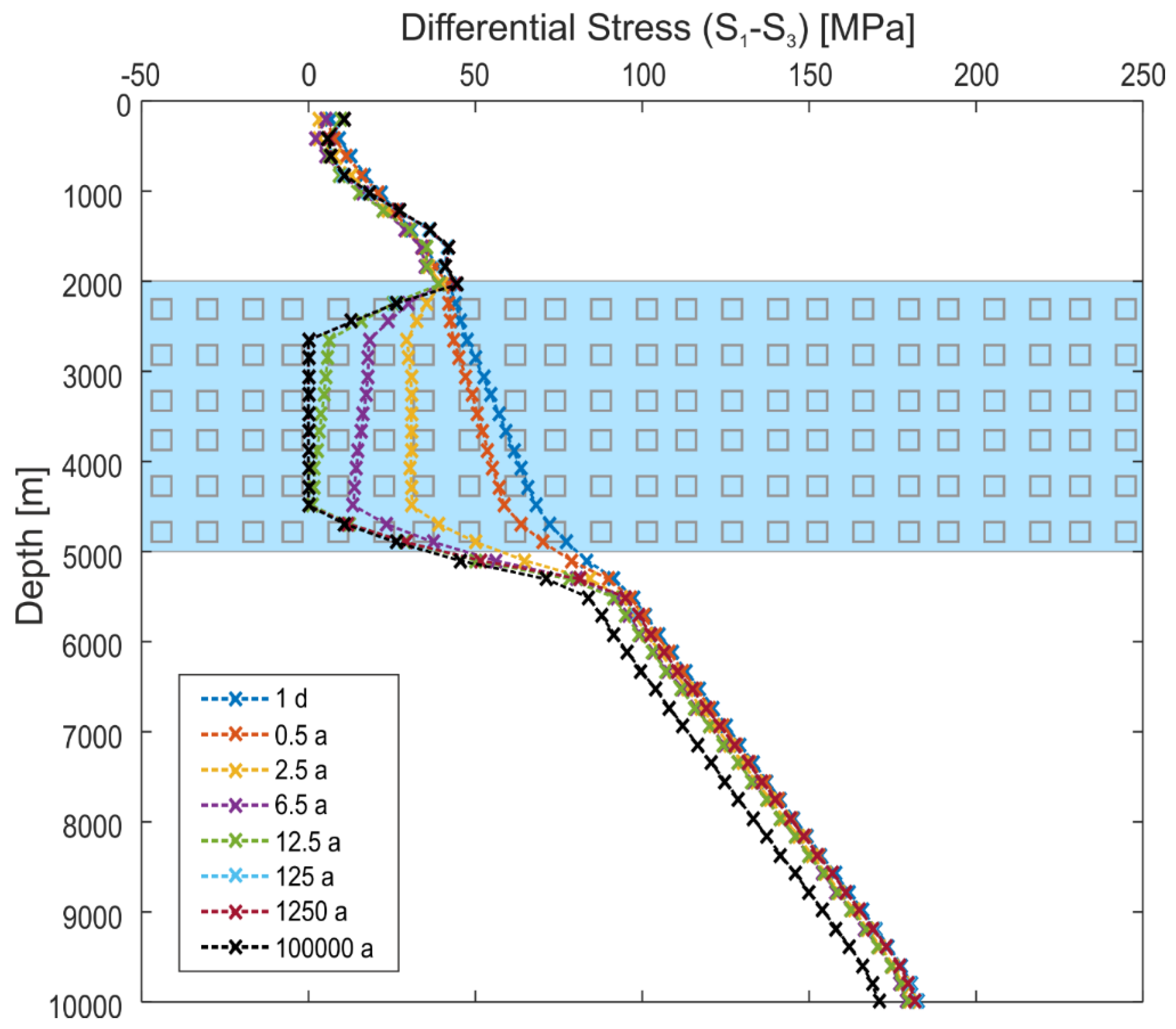
However, it should be noted that the decoupling is time-dependent. This means that decoupling does not always occur from the very beginning of the calculation, even for low viscosities. As an example, the temporal evolution of stress after the commencement of shortening in the subsalt section is shown in Figure 12 for Model B-04b. Changes of differential stress occur in all three sections (suprasalt, salt and subsalt). Within the salt, differential stress becomes very small after about 12.5 years, whereas after a few years only there is no full decoupling reached yet. The reduction of differential stress in the subsalt can be referred to the reduced difference between SV and Shmin, the latter being increased by shortening. Above the top of the diapir, differential stress evolves non-uniformly. Right above the top of the diapir, differential stress increases, whereas it decreases further upward.
In addition, our model results show that stress decoupling comprises not only vertical changes in the tectonic regime as in Model Series A, but causes also pronounced variability in the orientation of SHmax. For a viscosity of 1021 Pa·s this results from the superposition of the mechanical decoupling effects of the salt and deflections of the regional stress field due to the topology of the salt diapir. For the case of decoupling (salt viscosities lower than 1021 Pa·s), the stress field in the suprasalt is however only influenced by the interactions between the salt diapir and the surrounding suprasalt. This means, e.g., that the stress field in the suprasalt for the Model B-04c equals a suprasalt stress field for a model without subsalt shortening. The combined analysis of vertical and horizontal sections through the model domain shows that highly variable stress orientations can occur. For example, Figure 5 (Model B-04d and B-07b) indicates that S1 orientations are either parallel or perpendicular to the salt–sediment interface as the creeping salt cannot sustain any shear stresses. As a result, tilted stress fields occur in the vicinity of the salt body. For these parts of the model, the common assumption that one of the three principal stresses is vertical is not valid (See differences between SV, SHmax, Shmin and S1, S2, S3 in Figure 7 and Figure 8). Consequently, a description of the stress state therefore requires the complete stress tensor, i.e., the orientations and magnitudes of the three principal stress vectors. Another feature observed in the cross-sectional view is a small depression in the centre of the model, which is underlain by horizontal S1 orientations (Figure 5a and Figure 13). This depression can be explained by the lithostatic stress state within the salt diapir beneath, i.e., the magnitudes of horizontal stresses being equal to the vertical stress (e.g., Figure 7). Thus, horizontal stresses are higher in the salt than in the adjacent sediments, pushing the diapir’s walls outward against the sediments and, thereby, creating subsidence above. The effect of the density contrast across the flank of the diapir may add to the overall extensional stress field but it is not further investigated in this study. The small depression above the diapir and the outward movements are shown in Figure 13. The deformation of the purely elastic suprasalt material is likely not representative of the deformation of sedimentary rocks that can fail and deform plasticly. However, the stress field captured by these simplified models can help to understand the dynamics around salt–sediment contact. The stress field shows higher horizontal stresses (in extension direction) at the flank of the diapir (Figure 8) in contrast to the centre (Figure 7) and negative SV-Shmin values in the uppermost about 500 m, where the horizontal stress exceeds the vertical stress. Such negative stress differences of SV-Shmin are also observed in the uppermost ~1000 m of the NGB (Figure 1c). We like to emphasize that this stress difference is not the differential stress, which is defined as S1-S3 and can never be negative. The labelling in Figure 1c is often used by drilling engineers as a proxy for differential stress, as there is no better data available.
In the map view (Figure 6; Model B-04c), further depth-dependent deviations from the regional SHmax trend imposed by the salt topology become apparent. Three different patterns can be distinguished: a uniform, parallel SHmax orientation in the subsalt section, a radial pattern next to and immediately above the salt diapir and, finally, a circular pattern in the uppermost section, i.e., in the sediments above the salt diapir. The uniform pattern in the subsalt part simply reflects the boundary conditions imposed, i.e., displacements from the south. The radial pattern is a consequence of the close-to-lithostatic stress state in the salt diapir. There, the horizontal stresses have the same magnitude as Sv, which exceeds the horizontal stresses in the sediments surrounding the diapir (Figure 8). As a result, SHmax is oriented perpendicular to the diapir, which creates the radial patterns shown in Figure 6b,c. Such a radial pattern of SHmax in the vicinity of salt diapirs has also been described in the general case (e.g., by References [40,42,43]) and for special cases (e.g., for the North Sea [44]). The circular pattern and the rotation of SHmax by 90° in the uppermost suprasalt section can be explained by the same processes which also led to the formation of the small depression described above. The lithostatic stress state within the salt diapir leads to horizontal expansion of the salt diapir’s flanks while the sediments above are subsiding (Figure 13). This creates the stress orientation pattern observed in Figure 6d with circular SHmax orientations and Shmin radially pointing outward. A circular pattern of SHmax around salt diapirs has been found in the Gulf of Mexico where diapirs are surrounded by weak deltaic sediments contrary to our model assumptions [45,46]. Looking at the fault patterns around salt diapirs, these two stress fields are reflected there by radial and concentric fault patterns (e.g., described for the North Sea by [47,48] and for the general case by References [40,49,50]). Various analogue and numerical models address this relation between faults and the stress field, e.g., [51,52,53].
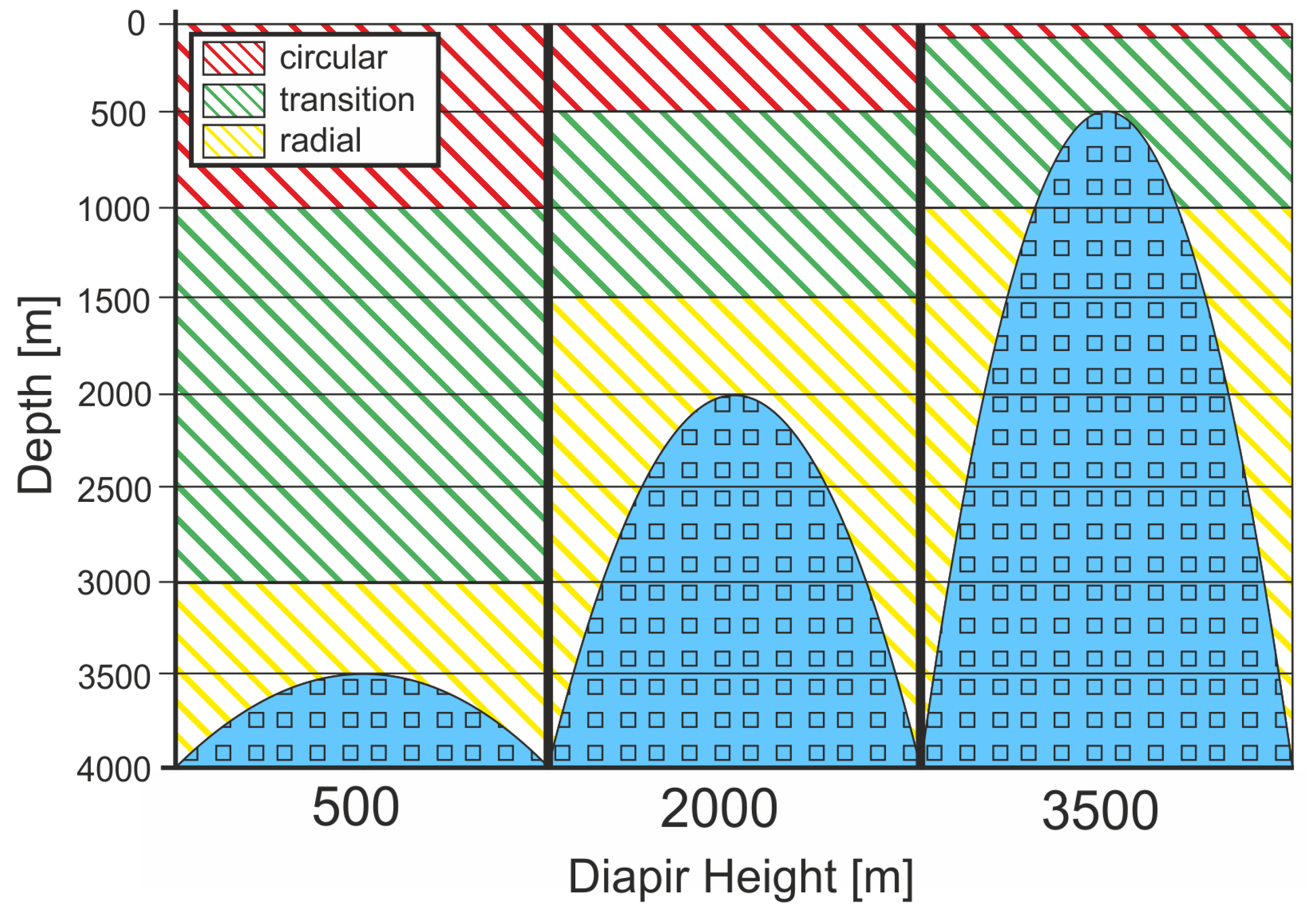
The depth interval where the switch from the radial to the circular pattern occurs, is found to depend on the height of the salt diapir (Figure 14). For a height of the salt diapir of 500 m (Model B-03), the transition from the radial to the circular pattern occurs between 500 and 2500 m above the diapir. For a 2000-m-high salt diapir (Model B-04a–B-04d), the rotation takes place between 500 m and 1500 m above the diapir, hence, within only half the vertical distance. The results for the diapir with a height of 3500 m (Model B-05) confirm this trend. The rotation already starts beneath the top of the diapir and shows the circular pattern ~500 m above. While the transition may take place within a narrower range at increased numerical resolution, this result nevertheless shows that the topology of the diapir affects the size of the depth interval above the diapir in which changes of the stress field can be expected.
Regarding depth-dependent variations in stress magnitude, the salt causes changes with respect to principal stress magnitudes as well as the stress difference Sv-Shmin. In the suprasalt section the modelled gradients are strongly influenced by the proximity to the salt diapir. Particularly above the salt diapir, SV-Shmin gradients of up to ~22.5 MPa/km have been modelled (Figure 9). This results from the decrease of the horizontal stresses in this part of the model (Figure 7). At distance from the salt diapir, lower stress gradients are encountered, also in case of the flat salt layer with ~18.5 MPa/km (Model A-02). In the sub- and suprasalt section, the modelled SV-Shmin gradients are higher than the data actually measured (Figure 1c). The average suprasalt gradient in the NGB is ~7.1 MPa/km and the subsalt gradient is ~11.4 MPa/km; our results suggest a gradient of ~20 MPa/km in the subsalt. The vertical stress in the model is essentially the weight of the overburden, therefore, this discrepancy can be explained by an underestimation of the horizontal stress magnitudes in the model. To overcome this discrepancy, lower SV-Shmin gradients would be obtained by applying higher shortening rates or by applying shortening over a longer period in order to increase horizontal stresses. However, geodetic observations do not provide evidence for higher shortening rates than about 1 mm/a as Central Europe is considered as a region of very low deformation rates. Observed rates with respect to an Eurasia Plate fixed reference system are in the range of measurement errors. This, however, does not exclude that accrued shortening in the past is still stored in the subsurface. As the aim of this study is the analysis of the conditions controlling mechanical decoupling we did not pursue this aspect further by considering the increase of the amount of shortening.
Regarding the effects of density, we tested a number of models with different density contrasts between salt and sediments (suprasalt) and found no significant differences in the resulting stress fields. This is probably due to our model setup and the fact that we do not consider bouyancy forces during the rise of the diapir.
The modelling results presented rely on a constant linear viscosity of the salt and show that the first-order pattern of stress redistribution in the suprasalt section of a sedimentary basin is subject to shortening in the basement. In reality, variable viscosities arising from (1) spatially variable salt mineralogy, which is common in subsequent evaporitic cycles [33], and (2) mechanisms involved in the deformation of salt such as dislocation creep [33] can be expected. These deformation mechanisms are commonly described by various types of non-linear relationships between the stress and strain rate and depend exponentially on temperature [32]. Such salt rheologies lead to (1) lower viscosities and, thus, higher strain rates in areas of higher temperature, and (2) higher strain rates in areas of high deviatoric stress. Thus, viscous deformation concentrates in particular areas. Applied to the models presented, non-linear viscosities would lead to spatial variations in strain, e.g., higher viscous strain (rates) in the lower part of the salt layer and the diapir, respectively.
5. Conclusions
We use a 3D finite element model to study the conditions leading to mechanical decoupling at a salt layer and vertically varying stress fields in salt-bearing sedimentary basins, respectively. The study was inspired by observational data from northern Germany, which shows stress orientations varying up to 90° between the subsalt and the suprasalt layers e.g., [12,16,18]. Even though the models do not incorporate the evolution of the salt diapir from a flat salt layer to its present-day shape, they provide valuable information on how the salt affects the contemporaneous stress field in the basin. The modelling work focused particularly on the role of salt viscosity and salt morphology and to what extent the recent plate boundary forces acting at the basement level also affect the stresses in the sedimentary cover above the salt layer.
The results of the modeling study can be summarised as follows:
- Stress decoupling is observed for dynamic salt viscosities of less than 1021 Pa·s at the assumed shortening rate of 4 × 10⁻¹⁶ s−1 and flat layer thickness of 1000 m. Larger viscosities foster mechanical coupling so that the stresses exerted only to the lower part of the model are transmitted to a shallower level, affecting also the stress field there.
- In case of mechanical decoupling, two independent stress fields exist above and below the salt layer which differ in tectonic stress regime and/or stress orientation. Thereby, stresses in the subsalt domain are dominated by the shortening applied, whereas in the suprasalt section they are controlled by the local salt topology.
- The orientation of SHmax above and in the vicinity of a salt diapir changes with increasing depth from a circular to a radial pattern. This reorientation is caused by the close-to-lithostatic stress state within the salt diapir, which leads to lateral expansion at the diapir’s flanks and subsidence above. In addition, the distance between the two stress patterns depends on the height of the diapir.
- The topology of the salt and the inability of the salt to sustain shear stress results in stress perturbations at the salt–sediment interface. Tilted stress fields can occur for which none of the principal stresses is oriented vertically.
- Regarding the NGB, modelling results show that uniform stress orientations below and very variable ones above the salt layer can coexist. Thus, the results are in broad agreement with the stress data actually observed. Models reproduce the negligible differential stresses within the salt layer, but some further tuning of the boundary conditions would be required to match also the stress gradients exactly.
Such a pronounced stress heterogeneity with stress orientations and magnitudes varying both laterally and vertically as indicated by the models can only occur in salt-bearing sedimentary basins. For basins without a mechanically weak decoupling layer, i.e., for those filled with siliciclastic and/or carbonate rocks only, the stress field orientation (apart from faults) is much more uniform and the plate boundary forces exerted at the basement level will be transmitted also to shallower levels. The study emphasises the value of geomechanical-numerical models as a tool for stress prediction in salt-bearing sedimentary basins. This approach, incorporating both the dynamic viscosity and the topology of the salt, can provide a continuum mechanics–based explanation for apparently conflicting stress observations.
Author Contributions
Conceptualization, A.H. and T.H.; Investigation, S.A. and T.H.; Methodology, S.A. and T.H.; Numerical models, S.A.; Visualization, S.A.; Writing—original draft preparation, S.A., T.H. and A.H.; Writing—review and editing, S.A., T.H. and A.H.; Project administration, A.H. and T.H.
Funding
This research received no external funding.
Acknowledgments
We thank two anonymous reviewers for helpful comments that improved the manuscript. We acknowledge support by the German Research Foundation and the Open Access Publishing Fund of Technische Universität Darmstadt.
Conflicts of Interest
The authors declare no conflict of interest.
References
- Tingay, M. State and origin of present-day stress fields in sedimentary basins. Australian Society of Exploration Geophysicists Extended Abstracts. In Proceedings of the Australian Society of Exploration Geophysicists 20th International Conference and Exhibition, Adelaide, Perth, 22 February 2009; Rod Lovibond, Ed.; CSIRO Publishing: Clayton, Australia, 2009. [Google Scholar]
- Heidbach, O.; Tingay, M.; Barth, A.; Reinecker, J.; Kurfeß, D.; Müller, B. Global crustal stress pattern based on the World Stress Map database release 2008. Tectonophysics 2010, 482, 3–15. [Google Scholar] [CrossRef] [Green Version]
- Lund Snee, J.-E.; Zoback, M.D. State of stress in Texas: Implications for induced seismicity. Geophys. Res. Lett. 2016, 43, 10208–10214. [Google Scholar] [CrossRef]
- Rajabi, M.; Tingay, M.; Heidbach, O.; Hillis, R.; Reynolds, S. The present-day stress field of Australia. Earth-Sci. Rev. 2017, 168, 165–189. [Google Scholar] [CrossRef]
- Bell, J.S. Petro geoscience 2. In situ stresses in sedimentary rocks (part 2): Applications of stress measurements. Geosci. Can. 1996, 23, 135–153. [Google Scholar]
- Yale, D.P. Fault and stress magnitude controls on variations in the orientation in situ stress. In Fracture and In-Situ Stress Characterization of Hydrocarbon Reservoirs; Ameen, M.S., Ed.; Geological Society of London: London, UK, 2003; pp. 55–64. [Google Scholar]
- Henk, A. Pre-drilling prediction of the tectonic stress field with geomechanical models. First Break 2005, 23, 53–57. [Google Scholar] [CrossRef]
- Fischer, K.; Henk, A. Modeling the Pre-Production Stress State in a Gas Reservoir—An Applied Workflow. Oil Gas Eur. Mag. 2014, 130, 190–195. [Google Scholar]
- Rajabi, M.; Tingay, M.; Heidbach, O. The present-day state of tectonic stress in the Darling Basin, Australia: Implications for exploration and production. Mar. Pet. Geol. 2016, 77, 776–790. [Google Scholar] [CrossRef]
- Rajabi, M.; Ziegler, M.; Tingay, M.; Heidbach, O.; Reynolds, S. Contemporary tectonic stress pattern of the Taranaki Basin, New Zealand. J. Geophys. Res. 2016, 121, 6053–6070. [Google Scholar] [CrossRef] [Green Version]
- Tingay, M.; Bentham, P.; de Feyter, A.; Kellner, A. Present-day stress-field rotations associated with evaporites in the offshore Nile Delta. GSA Bull. 2011, 123, 1171–1180. [Google Scholar] [CrossRef]
- Cornet, F.H.; Röckel, T. Vertical stress profiles and the significance of “stress decoupling”. Tectonophysics 2012, 581, 193–205. [Google Scholar] [CrossRef]
- Hübner, W.; Wellbrink, M.; Röckel, T.; Steuer, S.; Krug, S.; Tischner, T. Stress rotation in the suprasalt beneath Hanover (North German Basin) derived from image logs of the deep well Groß Buchholz Gt1. Z. Dtsch. Ges. Geowiss. 2015, 166, 361–373. [Google Scholar] [CrossRef] [PubMed]
- Williams, J.D.O.; Fellgett, M.W.; Kingdon, A.; Williamson, J.P. In-situ stress orientations in the UK Southern North Sea: Regional trends, deviations and detachment of the post-Zechstein stress field. Mar. Pet. Geol. 2015, 67, 769–784. [Google Scholar] [CrossRef] [Green Version]
- Hehn, R.; Genter, A.; Vidal, J.; Baujard, C. Stress field rotation in the EGS well GRT-1 (Rittershoffen, France). In European Geothermal Congress Conference Paper–2016; European Geothermal Congress: Strasbourg, France, 2016. [Google Scholar]
- Roth, F.; Fleckenstein, P. Stress orientations found in NE Germany differ from the West European trend. Terra Nova 2001, 13, 289–296. [Google Scholar] [CrossRef]
- Maystrenko, Y.; Bayer, U.; Brink, H.-J.; Littke, R. The Central European Basin system; an overview. In Dynamics of Complex Intracontinental Basins: The Central European Basin System; Littke, R., Bayer, U., Gajewski, D., Nelskamp, S., Eds.; Springer: Berlin/Heidelberg, Germany, 2008; pp. 15–34. [Google Scholar]
- Röckel, T.; Lempp, C. Der Spannungszustand im Norddeutschen Becken. Erdöl-Erdgas-Kohle 2003, 119, 73–80. [Google Scholar]
- Stollhofen, H.; Bachmann, G.H.; Barnasch, J.; Bayer, U.; Beutler, G.; Franz, M.; Kästner, M.; Legler, B.; Mutterlose, J.; Radies, D. Upper Rotliegend to early Cretaceous basin development. In Dynamics of Complex Intracontinental Basins: The Central European Basin System; Littke, R., Bayer, U., Gajewski, D., Nelskamp, S., Eds.; Springer: Berlin/Heidelberg, Germany, 2008; pp. 181–210. [Google Scholar]
- Warren, J.K. Salt as sediment in the Central European Basin System as seen from a deep time perspective. In Dynamics of Complex Intracontinental Basins: The Central European Basin System; Littke, R., Bayer, U., Gajewski, D., Nelskamp, S., Eds.; Springer: Berlin/Heidelberg, Germany, 2008; pp. 247–276. [Google Scholar]
- Pfiffner, O.A. Thick-skinned and thin-skinned tectonics: A global perspective. Geosciences 2017, 7, 71. [Google Scholar] [CrossRef]
- Lundin, E.R. Thin-skinned extensional tectonics on a salt detachment, northern Kwanza Basin, Angola. Mar. Pet. Geol. 1992, 9, 405–411. [Google Scholar] [CrossRef]
- Gemmer, L.; Ings, S.J.; Medvedev, S.; Beaumont, C. Salt tectonics driven by differential sediment loading: Stability analysis and finite-element experiments. Basin Res. 2004, 16, 199–218. [Google Scholar] [CrossRef]
- Ruh, J.B.; Kaus, B.J.P.; Burg, J.-P. Numerical investigation of deformation mechanics in fold-and-thrust belts: Influence of rheology of single and multiple décollements. Tectonics 2012, 31. [Google Scholar] [CrossRef]
- Hillis, R.R.; Nelson, E.J. In situ stresses in the North Sea and their applications: Petroleum geomechanics from exploration to development. In Proceedings of the 6th Petroleum Geology Conference Petroleum Geology: North-West Europe and Global Perspectives, London, UK, 6–9 October 2003; Dóre, A.G., Vining, B.A., Eds.; Geological Society: London, UK, 2005; pp. 551–564. [Google Scholar]
- Zienkiewicz, O.C.; Taylor, R.L. The Finite Element Method, 5th ed.; Butterworth-Heinemann: Oxford, UK, 2010. [Google Scholar]
- Scheck-Wenderoth, M.; Lamarche, J. Crustal memory and basin evolution in the Central European Basin System—New insights from a 3D structural model. Tectonophysics 2005, 397, 143–165. [Google Scholar] [CrossRef]
- Maystrenko, Y.P.; Bayer, U.; Scheck-Wenderoth, M. Salt as a 3D element in structural modeling—Example from the Central European Basin System. Tectonophysics 2013, 591, 62–82. [Google Scholar] [CrossRef]
- Fossen, H. Structural Geology, 3rd ed.; Cambridge University Press: Cambridge, UK, 2012. [Google Scholar]
- Jaeger, J.C.; Cook, N.G.W.; Zimmerman, R.W. Fundamentals of Rock Mechanics, 4th ed.; Blackwell Publishing: Malden, MA, USA; Oxford, UK; Carlton, ON, Canada, 2007. [Google Scholar]
- Abaqus. Abaqus 6.11 Documentation; Dassault Systèmes Simulia Corporation: Providence, RI, USA, 2011. [Google Scholar]
- Van Keken, P.E.; Spiers, C.J.; van den Berg, A.P.; Muyzert, E.J. The effective viscosity of rocksalt: Implementation of steady-state creep laws in numerical models of salt diapirism. Tectonophysics 1993, 225, 457–476. [Google Scholar] [CrossRef]
- Urai, J.L.; Schléder, Z.; Spiers, C.J.; Kukla, P.A. Flow and transport properties of salt rocks. In Dynamics of Complex Intracontinental Basins: The Central European Basin System; Littke, R., Bayer, U., Gajewski, D., Nelskamp, S., Eds.; Springer: Berlin/Heidelberg, Germany, 2008; pp. 277–289. [Google Scholar]
- Reyer, D.; Philipp, S.L. Empirical relations of rock properties of outcrop and core samples from the Northwest German Basin for geothermal drilling. Geotherm. Energy Sci. 2014, 2, 21–37. [Google Scholar] [CrossRef] [Green Version]
- Turcotte, D.L.; Schubert, G. Geodynamics, 3rd ed.; Cambridge University Press: Cambridge, UK, 2014. [Google Scholar]
- Braeuer, V.; Eickemeier, R.; Eisenburger, D.; Grissemann, C.; Hesser, J.; Heusermann, S.; Kaiser, D.; Nipp, H.-K.; Nowak, T.; Plischke, I.; et al. Standortbeschreibung Gorleben Teil 4. Geotechnische Erkundung des Salzstocks Gorleben; Schweizerbart Science Publishers: Stuttgart, Germany, 2012. [Google Scholar]
- Marotta, A.M.; Bayer, U.; Thybo, H.; Scheck, M. Origin of the regional stress in the North German Basin–results from numerical modelling. Tectonophysics 2002, 360, 245–264. [Google Scholar] [CrossRef]
- Kaiser, A.; Reicherter, K.; Huebscher, C.; Gajewski, D.; Marotta, A.M.; Bayer, U. Variation of the present-day stress field within the North German Basin; insights from thin shell FE modeling based on residual GPS velocities. Tectonophysics 2005, 397, 55–72. [Google Scholar] [CrossRef]
- Bjørlykke, K. Effects of compaction processes on stresses, faults, and fluid flow in sedimentary basins: Examples from the Norwegian margin. In Analogue and Numerical Modelling of Crustal-Scale Processes; Bujter, S.J.H., Schreuers, G., Eds.; Geological Society: London, UK, 2006; pp. 359–379. [Google Scholar]
- Dusseault, M.B.; Maury, V.; Sanfilippo, F.; Santarelli, F.J. Drilling Around Salt: Risks, Stresses, and Uncertainties. In Proceedings of the 6th North America Rock Mechanics Symposium (NARMS), Gulf Rocks Houston, TX, USA, 5–6 June 2004; ARMA Conference Paper–2004; American Rock Mechanics Association: Alexandria, VA, USA, 2004. [Google Scholar]
- Reiter, K.; Heidbach, O.; Müller, B.; Reinecker, J.; Röckel, T. Spannungskarte Deutschland 2016. GFZ Data Serv. 2016. [Google Scholar] [CrossRef]
- Luo, G.; Nikolinakou, M.A.; Flemings, P.B.; Hudec, M.R. Geomechanical modeling of stresses adjacent to salt bodies; Part 1, Uncoupled models. AAPG Bull. 2012, 96, 43–64. [Google Scholar] [CrossRef]
- Nikolinakou, M.A.; Hudec, M.R.; Flemings, P.B. Comparison of evolutionary and static modeling of stresses around a salt diapir. Mar. Pet. Geol. 2014, 57, 537–545. [Google Scholar] [CrossRef]
- Schutjens, P.M.T.M.; Snippe, J.R.; Mahani, H.; Turner, J.; Ita, J.; Mossop, A.P. Production-induced stress change in and above a reservoir pierced by two salt domes: A geomechanical model and its applications. SPE J. 2012, 17, 80–97. [Google Scholar] [CrossRef]
- King, R.; Backé, G.; Tingay, M.; Hillis, R.; Mildren, S. Stress deflections around salt diapirs in the Gulf of Mexico. In Faulting, Fracturing and Igneous Intrusion in the Earth’s Crust; Healy, D., Sibson, R.H., Shipton, Z., Butler, R., Eds.; Geological Society: London, UK, 2012; pp. 141–153. [Google Scholar]
- Yassir, N.A.; Zerwer, A. Stress regimes in the Gulf coast, offshore Louisiana: Data from well-bore breakout analysis. AAPG Bull. 1997, 81, 293–307. [Google Scholar]
- Davison, I.; Alsop, G.I.; Evans, N.G.; Safaricz, M. Overburden deformation patterns and mechanisms of salt diapir penetration in the Central Graben, North Sea. Mar. Pet. Geol. 2000, 17, 601–618. [Google Scholar] [CrossRef]
- Carruthers, D.; Cartwright, J.; Jackson, M.P.A.; Schutjens, P. Origin and timing of layer-bound radial faulting around North Sea salt stocks: New insights into the evolving stress state around rising diapirs. Mar. Pet. Geol. 2013, 48, 130–148. [Google Scholar] [CrossRef]
- Stewart, S.A. Implications of passive salt diapir kinematics for reservoir segmentation by radial and concentric faults. Mar. Pet. Geol. 2006, 23, 843–853. [Google Scholar] [CrossRef]
- Quinta, A.; Tavani, S.; Roca, E. Fracture pattern analysis as a tool for constraining the interaction between regional and diapir-related stress fields: Poza de la Sal Diapir (Basque Pyrenees Spain). In Salt Tectonics, Sediments and Prospectivity; Archer, S.G., Alsop, G.I., Hartley, A.J., Grant, N.T., Hodgkinson, R., Eds.; Geological Society: London, UK, 2012; pp. 521–532. [Google Scholar]
- Withjack, M.O.; Scheiner, C. Fault Patterns Associated with Domes—An experimental Study. AAPG Bull. 1982, 66, 302–316. [Google Scholar]
- Yin, H.; Groshong, R.H., Jr. A three-dimensional kinematic model for the deformation above an active diapir. AAPG Bull. 2007, 91, 343–363. [Google Scholar] [CrossRef]
- Yin, H.; Zhang, J.; Meng, L.; Liu, Y.; Xu, S. Discrete element modeling of the faulting in the sedimentary cover above an active salt diapir. J. Struct. Geol. 2009, 31, 989–995. [Google Scholar] [CrossRef]
Figure 1.
Observed stress orientations and magnitudes in the North German Basin (NGB). (a) Orientation of the maximum horizontal Stress (SHmax) (black bars) above and (b) below the Zechstein stratigraphic unit in part of the NGB (modified after [16]). (c) Magnitudes of SV-Shmin-vertical stress (SV) minus minimum horizontal stress (Shmin)—from borehole measurements in the eastern part of the NGB. The blue line corresponds to the Zechstein (salt) layer, the red triangles to the subsalt and the green triangles to the suprasalt (simplified after [12]).

Figure 2.
Model set-up. (a) Geometry and finite element grid of Model Series B with three layers and central salt diapir (which does not exist in Model Series A). (b) Sketch showing a vertical section through the model and the boundary conditions applied (not to scale). (c) Horizontal section through the central part of the model at a depth of 3000 m. P marks the position of a vertical profile through the model and parallel to the shortening direction (as shown in b), while W1–W3 are the sites of hypothetical vertical wells. P and W1–W3 are used to present modelling results as vector diagrams and stress vs. depth plots, respectively.

Figure 3.
Orientation of the maximum stress (S1) along a vertical section through the centre of a model with a flat salt layer (in blue; see P in Figure 2c) for two different dynamic salt viscosities. Shortening amounts to 400 m and is applied to the subsalt section on the left. (a) For a salt viscosity of 1016 Pa·s (Model A-01), S1 is vertical in the suprasalt and horizontal in the subsalt region. This also implies a change in the tectonic regime—a normal faulting regime in the upper part and a strike-slip regime in the lower part of the model domain. (b) For a salt viscosity of 1024 Pa·s (Model A-03), S1 is horizontal in the supra- and most of the subsalt section in spite of the velocity boundary condition being applied to the subsalt part of the model only. Hence, the tectonic regime is largely uniform throughout the model.

Figure 4.
Differential stress (S1–S3) for a model with a salt viscosity of 1018 Pa·s (Model A-02) along a vertical path through the centre of the model (equivalent to a hypothetical well; see W1 in Figure 2c). The blue layer marks the depth interval of the salt. Within the salt layer, differential stresses essentially vanish.

Figure 5.
Orientation of S1 along a vertical section (see P in Figure 1c) through the centre of a model with a salt diapir (x = 40000 m) for two different dynamic viscosities of the salt (blue layer). Shortening amounts to 400 m and is applied to the subsalt on the left. (a) Viscosity of 1018 Pa·s (Model B-04d); S1 is mainly vertical in the suprasalt and horizontal in the subsalt region. Some stress perturbations are observed in the suprasalt section near the top of the salt layer and above the diapir. (b) Viscosity of 1021 Pa·s (Model B-07b); in comparison to (a), larger parts of the model in the suprasalt domain are characterised by a horizontal orientation of S1.

Figure 6.
Four horizontal sections through the central part of Model B-04c showing the orientation of SHmax. (a) at 10000 m depth, below the salt; (b) at 3500 m depth at about the middle of the salt diapir marked by the blue circular cross section; (c) at 1500 m depth right above the top of the salt diapir; and (d) at 500 m depth. Shortening amounts to 200 m and is applied to the subsalt (below 5000 m) in y-direction. Salt viscosity is 1018 Pa·s.

Figure 7.
Principal stress magnitudes for a hypothetical well (see W1 in Figure 2c) located in the centre of the model and of the salt diapir, respectively. Results are for Model B-04c, i.e., a salt diapir of 2000 m height, a salt viscosity of 1018 Pa·s and 200 m of shortening in the subsalt section. The blue layer marks the depth interval covered by the salt diapir.

Figure 8.
Principal stress magnitudes for two hypothetical wells (W2 and W3) in the northern flank of the diapir of Model B-04c (Figure 2c). (a) W2—1500 m north of W1 in the middle of the diapir flank. (b) W3—3000 m north of W1 and 1500 m north of (a) at the lower edge of the diapir flank.
Figure 8.
Principal stress magnitudes for two hypothetical wells (W2 and W3) in the northern flank of the diapir of Model B-04c (Figure 2c). (a) W2—1500 m north of W1 in the middle of the diapir flank. (b) W3—3000 m north of W1 and 1500 m north of (a) at the lower edge of the diapir flank.

Figure 9.
Stress difference SV-Shmin for five different salt viscosities ranging from 1016 to 1024 Pa·s. Stresses are plotted along a vertical well path through the centre of the salt diapir (see W1 in Figure 2c) for Models B-01, B-04c, B-06, B-08 and B-09. SV-Shmin of Model B-01 (1016 Pa·s) is hard to see as it is almost identical to Model B-04c (1018 Pa·s). The blue layer marks the depth interval covered by the salt diapir.

Figure 10.
Frequency distribution of SHmax orientations at different depths and for different viscosities. An orientation of 0° corresponds to a N–S strike of SHmax, which is the direction of shortening applied to the model boundary. Negative values indicate a counterclockwise rotation of SHmax towards the west, whereas positive angles show clockwise rotation towards the east. (a) Salt viscosity is 1018 Pa·s (Model B-04c). (b) Salt viscosity is 1021 Pa·s (Model B-07a).

Figure 11.
Frequency distribution of SHmax orientations at 3500 m depth for different viscosities (Models B-04c and B-07a) and in case of additional shortening in the suprasalt section by half the amount applied to the subsalt unit (Model B-02).
Figure 11.
Frequency distribution of SHmax orientations at 3500 m depth for different viscosities (Models B-04c and B-07a) and in case of additional shortening in the suprasalt section by half the amount applied to the subsalt unit (Model B-02).

Figure 12.
Differential Stress (S1–S3) after different total times for Model B-04b along the hypothetical well W1 (Figure 2). The blue line corresponds to the total time after the initial increment of 1 × 10⁵ s and the black line to the total time after the last increment (3.154 × 10¹² s). All times are roughly rounded.

Figure 13.
Vertical and lateral movements along the hypothetical wells W1–W3 (See Figure 2c). The red line crosses show the movement in y-direction. The blue line and crosses show the relative surface movement related to the average subsidence of the whole model for Model B-04a.
Figure 13.
Vertical and lateral movements along the hypothetical wells W1–W3 (See Figure 2c). The red line crosses show the movement in y-direction. The blue line and crosses show the relative surface movement related to the average subsidence of the whole model for Model B-04a.

Figure 14.
Distribution of the pattern of SHmax around and above the salt diapir with regard to the diapir height (Model B-03–B-05). The yellow hatched areas show the radial pattern (e.g., Figure 6b), the red hatched areas show the circular pattern (e.g., Figure 6d) and the green hatched areas show the transition zone between these two patterns.


Table 1.
Overview of model variants.
| Model | Viscosity (Pa·s) | Amount of Shortening (m) | Shortened Layer(s) | Height of Diapir (m) | Figure(s) | |
|---|---|---|---|---|---|---|
| Series A (flat salt layer) | A-01 | 1016 | 400 | Subsalt | - | 3a |
| A-02 | 1018 | 200 | Subsalt | - | 4 | |
| A-03 | 1024 | 400 | Subsalt | - | 3b | |
| Series B (salt layer with diapir) | B-01 | 1016 | 200 | Subsalt | 2000 | 9 |
| B-02 | 1018 | 200 (100) | Sub- and Suprasalt | 2000 | 11 | |
| B-03 | 1018 | 200 | Subsalt | 500 | 14 | |
| B-04a | 1018 | 0 | Subsalt | 2000 | 13 | |
| B-04b | 1018 | 100 | Subsalt | 2000 | 12 | |
| B-04c | 1018 | 200 | Subsalt | 2000 | 6,7,8,9,10,11,14 | |
| B-04d | 1018 | 400 | Subsalt | 2000 | 5a | |
| B-05 | 1018 | 200 | Subsalt | 3500 | 14 | |
| B-06 | 1020 | 200 | Subsalt | 2000 | 9 | |
| B-07a | 1021 | 200 | Subsalt | 2000 | 10,11 | |
| B-07b | 1021 | 400 | Subsalt | 2000 | 5b | |
| B-08 | 1022 | 200 | Subsalt | 2000 | 9 | |
| B-09 | 1024 | 200 | Subsalt | 2000 | 9 |
© 2018 by the authors. Licensee MDPI, Basel, Switzerland. This article is an open access article distributed under the terms and conditions of the Creative Commons Attribution (CC BY) license (http://creativecommons.org/licenses/by/4.0/).
Share and Cite
MDPI and ACS Style
Ahlers, S.; Hergert, T.; Henk, A. Numerical Modelling of Salt-Related Stress Decoupling in Sedimentary Basins–Motivated by Observational Data from the North German Basin. Geosciences 2019, 9, 19. https://doi.org/10.3390/geosciences9010019
AMA Style
Ahlers S, Hergert T, Henk A. Numerical Modelling of Salt-Related Stress Decoupling in Sedimentary Basins–Motivated by Observational Data from the North German Basin. Geosciences. 2019; 9(1):19. https://doi.org/10.3390/geosciences9010019
Chicago/Turabian StyleAhlers, Steffen, Tobias Hergert, and Andreas Henk. 2019. "Numerical Modelling of Salt-Related Stress Decoupling in Sedimentary Basins–Motivated by Observational Data from the North German Basin" Geosciences 9, no. 1: 19. https://doi.org/10.3390/geosciences9010019
Note that from the first issue of 2016, this journal uses article numbers instead of page numbers. See further details here.