Simulations of Fine-Meshed Biaxial Tests with Barodesy

Abstract

Recent experimental studies showed that shear band development starts at the beginning of triaxial tests. In experimental testing, it is impossible to obtain a soil sample with a homogeneous void ratio. Therefore, a homogeneous deformation, i.e., an element test, is questionable well before the peak. In this article we carry out finite element simulations of fine-meshed biaxial tests with the constitutive model barodesy, where the stress rate is formulated as a function of stress, stretching and void ratio. The initial void ratio in the simulations is normally distributed over all elements in a narrow range. In this article, we evaluate the pre-peak shear band development. We further compare stress paths and stress-strain curves of the biaxial test of relevant elements (e.g., in- and outside the shear band) with the results of the average response of all elements. We show how the response in an element test differs from the average response of the fine-meshed test. We present the resulting potential for understanding (early) shear band development and stress-strain behaviour in a biaxial test: The inhomogeneous void ratio distribution in a sample favours early shear band development. This effect is modelled with barodesy. The obtained stress paths and stress-strain curves show that the maximum deviatoric stress is higher in the element test than it is in the average response of the fine-meshed test.

1. Introduction

Soil is a material which consists of different grain sizes and grain shapes. The density or void ratio in a soil sample is naturally scattered and is thus not constant. Even for an ideal material consisting of spheres of the same size, inhomogeneities are to be expected due to inhomogeneous sample mounting. Experiments, e.g., triaxial tests, are carried out to investigate soil behaviour. In the evaluation of stress and strain, it is common to assume the sample to be a single homogeneous element with rectilinear deformation. In experimental testing, however, it is impossible to obtain a completely homogeneous sample with constant void ratio. In addition, the deformation of the sample in the experiment is not rectilinear: lateral barreling of the sample and/or development of shear band(s) are observed.

Finite element simulations on homogeneous samples lead to homogeneous deformations and not to development of shear bands. However, the pronounced localization in a biaxial test results in different stress-strain curves in- and outside the shear band. Thus, a single element test obviously cannot reproduce a realistic stress-strain response, e.g., [1]. To obtain shear bands, at least one weak element must be included in the simulation, e.g., [2,3,4]. Tomographic investigations on experiments by Desrues et al. [5] show that shear bands develop from the very beginning of triaxial tests. Therefore, a homogeneous deformation, i.e., an element test, is questionable well before the peak.

We perform finite element simulations of fine-meshed biaxial tests with barodesy [6]. Barodesy is a material model which includes the void ratio as a state variable. In this article, the initial void ratio is normally distributed over all elements in a narrow range, comparable to [7]. Thus, the natural scattering of density is modelled. The randomly distributed void ratio leads to a scatter of dilatancy and therefore in a scatter of peak strength in the elements. Hence, patterns of shear bands develop from the very beginning of the biaxial test. We evaluate stress-strain curves, stress paths and the pattern of the shear bands with ongoing deviatoric strain [8].

The innovative part of this research is to scatter the void ratio in combination with an evaluation of the average response of stress and strain of the fine-meshed test. The aim of this work is to find out whether and in which cases the approximation of a soil sample by a single element is justified and valid. In this context, it is possible to distinguish what has to be modelled by the constitutive relation and what by the numerical approach. We therefore compare the different response of a single element test with the average response of a fine-meshed test.

2. Material and Methods

2.1. Constitutive Model—Barodesy

Barodesy is a material model that differs from conventional elasto-plastic models: it does not distinguish between elastic and plastic deformations and does not require expressions such as yield function, plastic potential or flow rule. The stress rate is formulated as a tensorial function of the current stress, stretching and the void ratio, i.e., $\mathring{\sigma }=\mathbf{h}(\sigma ,\mathbf{D},e)$. Thus, barodesy has certain similarities with hypoplasticity [9,10]. Appendix A summarizes all equations of barodesy.

2.1.1. Critical State Soil Mechanics

The following concepts from Critical State Soil Mechanics are included in the mathematical formulation of barodesy [6]:

• A critical stress state locus [11,12], which is a line, the Critical State Line (CSL), in the $p^{\prime }$-q plot:

  $$q=M·p^{\prime }$$

  (1)

  with $M=6sin{\phi }_c/(3-sin{\phi }_c)$ for axisymmetric triaxial compression, ${\phi }_c$ is the critical friction angle. In three dimensional stress space, the critical stress locus of barodesy practically coincides with the Matsuoka–Nakai failure criterion [11], see Figure 1.
• A stress dependent critical void ratio $e_c$ (CSL from [13]) in the $p^{\prime }$-e plot, in order to distinguish between normally to slightly overconsolidated soil ($e>e_c$) and highly overconsolidated soil ($e<e_c$):

  $$ln(1+e_c)=N-{\lambda }^{*}ln\frac{2p^{\prime }}{{\sigma }^{*}}.$$

  (2)
• The isotropic normal compression line (NCL) from [14], in order to define the loosest possible packing:

  $$ln(1+e)=N-{\lambda }^{*}ln\frac{p^{\prime }}{{\sigma }^{*}},$$

  (3)

  ${\sigma }^{*}=1$ kPa is a reference stress, N and ${\lambda }^{*}$ are soil parameters from Critical State Soil Mechanics.

Further details of the mathematical formulation of barodesy are given in [6,12,15,16,17,18,19]. For the calibration procedure, we refer to [6].

2.1.2. Barotropy and Pyknotropy

By including the actual void ratio e as a state variable in barodesy, effects such as pyknotropy (i.e., the dependence of stiffness and strength on density) and barotropy (i.e., the dependence of stiffness and strength on stress level) can be modelled. In Figure 2 consolidated drained (CD) triaxial tests with Weald clay (parameters in

Table 1. Critical state soil mechanics parameters used for the calibration of barodesy.

Material	${\mathit{\phi }}_{\mathit{c}}$	N	${\mathit{\lambda }}^{*}$	${\mathit{\kappa }}^{*}$	Source
Weald clay	24${}^{\circ }$	0.8	0.059	0.018	Mašín [10]

) with the initial void ratio $e_{\mathrm{ini}}=$ const are simulated with barodesy. Highly overconsolidated samples (grayed area) dilate, normally and slightly overconsolidated samples contract, see Figure 2a. The stress states and the void ratios then reach the critical state. Highly overconsolidated samples achieve higher peak friction angles than the critical friction angle. The stress states reach the CSL after softening.

Similar results are obtained if the mean stress $p^{\prime }$ is kept constant and the void ratio is varied: In Figure 3 consolidated drained (CD) triaxial tests with Weald clay with $p_{\mathrm{ini}}^{\prime }=$ const are simulated with barodesy. The highly overconsolidated samples dilate, the normally and slightly overconsolidated samples contract, see Figure 3b. The lower the initial void ratio is, the higher is the maximum deviatoric stress q, see Figure 3b. Again the highly overconsolidated samples reach peak friction angles that are larger than the critical friction angle of ${24}^{\circ }$, see Figure 3c.

2.2. Biaxial Tests

We simulate drained plane strain triaxial compression (biaxial) tests, i.e., ${\epsilon }_2=0$ and ${\sigma }_3^{\prime }=100$ kPa = const. Biaxial tests on Weald clay with different overconsolidation ratios are investigated. The parameters of Weald clay are in Table 1. It is common to define the overconsolidation ratio (OCR = $p_e^{\prime }/p^{\prime }$) by means of the so-called Hvorslev’s equivalent consolidation pressure $p_e^{\prime }=exp\left(\frac{N-ln(1+e)}{{\lambda }^{*}}\right)$, divided by the actual mean stress $p^{\prime }$. $p_e^{\prime }$ is the value of mean stress on the isotropic normal consolidation line which refers to the current specific volume $(1+e)$.

2.2.1. Initial Conditions

We simulate biaxial tests, with a width of 37 mm and a height of 74 mm, see Figure 4a. Multiple elements and the stress boundary condition (${\sigma }_3^{\prime }=$ const) allow barreling of the sample in direction 3. The shear band thickness in finite element simulations is mesh-dependent, as the mesh serves as an internal length parameter, e.g., [20]. As the stress-strain curves in- and outside the shear band differ, the thickness certainly has an effect on the average response, see [21,22] and Figure 4b,c.

Gylland et al. [23] report about shear band thicknesses in the range of 2 to 8 mm for clay. In our simulations, the number elements (5000) have been chosen in a way that the final shear band thickness is in the reported range. In Figure 4b the final shear band is about 3 mm. By determining the preferred shear band thickness, we expect realistic predictions in the average response of strain and strain. This approach is only applicable for small dimensions due to the large number of elements. To overcome the mesh-dependency, a regularization technique is required [2,20,21].

The simulations in this work are carried out with abaqus 6.14 [24]. Four-node plane strain elements are used, see Figure 4b. The umat of barodesy [6] is available at SoilModels [25]. Finite element applications with barodesy can be found in [4,26,27].

In our simulations the initial void ratio is randomly and normally distributed over all 5000 elements in a narrow range (The standard deviation in our simulations is 0.005. In the simulations by Schneider-Muntau et al. [3], one weak element with an increased void ratio of 0.02 was included to obtain a shear band.) for different overconsolidation ratios according to

Table 2. Initial conditions for the FE simulations.

	OCR	Mean Value ${\overline{\mathit{e}}}_{\mathbf{ini}}$	Standard Deviation	${\mathit{p}}_{\mathbf{ini}}^{\prime }$
	1.5	0.656	0.005	100 kPa
	3	0.590	0.005	100 kPa
	6	0.526	0.005	100 kPa
	54	0.340	0.005	100 kPa

.

For an OCR of 6, the void ratio distribution is shown in Figure 5a. The mean value of ${\overline{e}}_{\mathrm{ini}}=0.526$ is marked with a black line. The red lines show the standard deviation, i.e., ${\overline{e}}_{\mathrm{ini}}\pm 0.005$. In order to better estimate the size of this standard deviation, we mark ${\overline{e}}_{\mathrm{ini}}$ and ${\overline{e}}_{\mathrm{ini}}\pm 0.005$ in the mean stress—void ratio plot with black and red lines in Figure 5b.

2.2.2. Evaluation of Stress Paths in the Deviatoric Plane

The deviatoric direction of a stress path is indicated by the Lode angle ${\alpha }_{\sigma }$, Equation (4):

$$\begin{array}{ccc}\hfill {\alpha }_{\sigma }& ={\displaystyle \frac{1}{3}}arcsin{\displaystyle \frac{-3\sqrt{6}det{\sigma }^{*}}{|{\sigma }^{*}{|}^3}}\mathrm{with}{\sigma }^{*}& =\sigma -\frac{tr\sigma }{3}\mathbf{1}\hfill \end{array}$$

(4)

${\alpha }_{\sigma }={30}^{\circ }$ refers to triaxial compression, ${\alpha }_{\sigma }=-{30}^{\circ }$ refers to triaxial extension. Nakai [28] reports that stress paths of plane strain conditions lie within $0^{\circ }<{\alpha }_{\sigma }<{15}^{\circ }$. The experimental findings by Nakai have been carried out on normally consolidated Fujinomori clay. However, the values also provide an indication for overconsolidated samples. Investigations under plane strain conditions were carried out with barodesy in [12,26].

2.2.3. Evaluation of the Inclination of Final Shear Band

The higher the overconsolidation ratio is, the steeper is the inclination of the final shear band. In barodesy, for a higher overconsolidation ratio there is a higher dilatancy and thus a higher mobilized friction angle, see Figure 3. The angle of dilatancy $\psi$ under plane strain conditions (e.g., [29]) is

$$\psi =arcsin{\displaystyle \frac{{\dot{\epsilon }}_1+{\dot{\epsilon }}_3}{-{\dot{\epsilon }}_1+{\dot{\epsilon }}_3}}.$$

(5)

The orientation of the shear band is reported (e.g., [23,30]) to lie between Roscoe’s solution [31] with

$${\theta }_{\mathrm{R}}={45}^{\circ }+\psi /2$$

(6)

and the Mohr-Coulomb solution with

$${\theta }_{\mathrm{M}C}={45}^{\circ }+{\phi }_m^{\max }/2.$$

(7)

Arthur et al. [32] propose

$${\theta }_{\mathrm{A}}=\frac{1}{2}({\theta }_{\mathrm{M}C}+{\theta }_{\mathrm{R}})$$

(8)

based on their experimental results. The angle $\psi$ in Equations (6) and (7) is the angle of dilatancy at the peak of q. ${\phi }_m^{\max }$ is the maximum mobilized friction angle, which is for the simulations in this article at the peak of q.

3. Results

In this Section we evaluate the simulations of fine-meshed biaxial tests. The results of the overconsolidation ratios 1.5, 3, 6 and 54 are discussed. We focus on early shear band development, stress-strain behaviour, stress paths in the deviatoric plane and inclination of the final shear band. All simulations are carried out with the material model barodesy [6]. Further details concerning the model are in Section 2.1. Information about the initial conditions and evaluation of the biaxial tests are in Section 2.2.

3.1. Early Shear Band Development

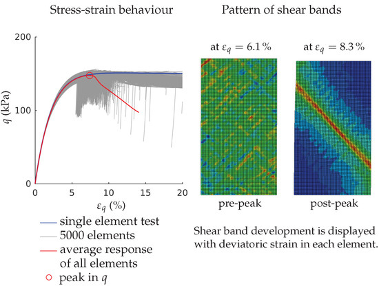
In Figure 6, Figure 7, Figure 8 and Figure 9 we show the development of shear bands at different global deviatoric strain ${\epsilon }_q$. Figure 6 corresponds to an OCR of 1.5, Figure 7 to an OCR of 3, Figure 8 to an OCR of 6 and Figure 9 to an OCR of 54. For all overconsolidation ratios, it is visible that shear bands develop well before the peak. The peak state is marked in the figures or figures captions. For example, Figure 6a–c show pre-peak pattern of shear bands, (d) is just at peak state and (e,f) show the final shear band. As expected, the smaller the OCR, the more pronounced is the barreling of the sample. For all OCRs a final shear band develops. The development of the final shear band has a strong influence on the shape of the average response of the stress-strain curve, especially in the post-peak range.

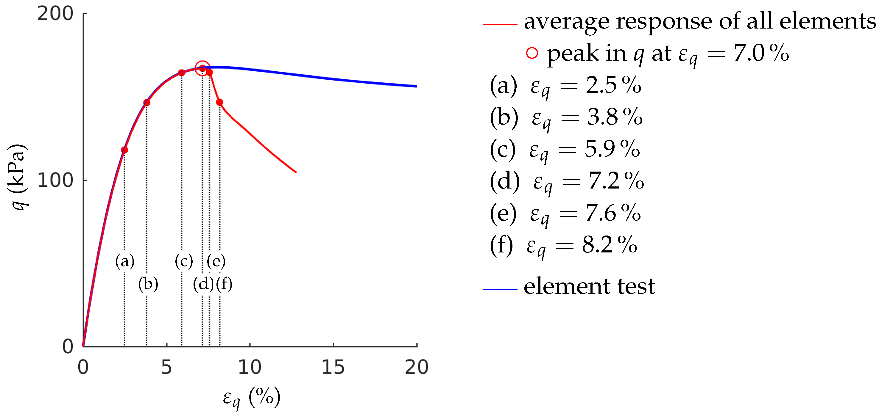
In Figure 10, Figure 11, Figure 12 and Figure 13 the result of an element test (blue), as well as the average response of the fine-meshed test (red) are shown for the OCRs of 1.5, 3, 6 and 54. The average densities of the fine-meshed biaxial test and the single element test coincide for each OCR. The global deviatoric strain corresponding to Figure 6, Figure 7, Figure 8 and Figure 9 is marked in Figure 10, Figure 11, Figure 12 and Figure 13. In Figure 10, the average response of the fine-meshed test (red) and the element test (blue) give similar results until ${\epsilon }_q\approx 8\%$. An overconsolidation of 1.5 corresponds to a slightly overconsolidated specimen. Therefore, the element test does not show any softening. It is interesting to note that the average response of the fine-meshed test has a peak with subsequent softening. Biaxial tests on loose Hostun sand samples [33] show a similar stress-strain behaviour. For all OCRs, the peak and subsequent softening is more pronounced in the average response of the fine-meshed test than it is in the element test.

In the element test, the maximum deviatoric stress is higher than in the fine-meshed test. The lower the initial overconsolidation ratio is, the larger is the difference, see

Table 3. Maximum deviatoric stress $q^{\max }$ in the element test and in the average response of all elements and maximum mobilized friction angles ${\phi }_m^{\max }$ in the element test and in the average response of all elements.

OCR	${\mathit{q}}^{\mathbf{max}}$		Difference in q	${\mathit{\phi }}_{\mathit{m}}^{\mathbf{max}}$		Difference in ${\mathit{\phi }}_{\mathit{m}}$
	Element Test	FE		Element Test	FE
1.5	$149.46$ kPa	$136.32$ kPa	$9.64\%$	${27.43}^{\circ }$	${25.86}^{\circ }$	$6.07\%$
3	$151.05$ kPa	$147.57$ kPa	$2.36\%$	${27.62}^{\circ }$	${27.23}^{\circ }$	$1.43\%$
6	$167.61$ kPa	$166.88$ kPa	$0.44\%$	${29.33}^{\circ }$	${29.40}^{\circ }$	$0.24\%$
54	$241.38$ kPa	$240.50$ kPa	$0.37\%$	${35.44}^{\circ }$	${35.37}^{\circ }$	$0.18\%$

. For the OCR of 1.5, the difference is $9.64\%$ and for the OCR of 54, $0.37\%$. In Table 3 the maximum mobilized friction angles ${\phi }_m^{\max }$ in the element tests and in the average response of all elements are added for the different overconsolidation ratios.

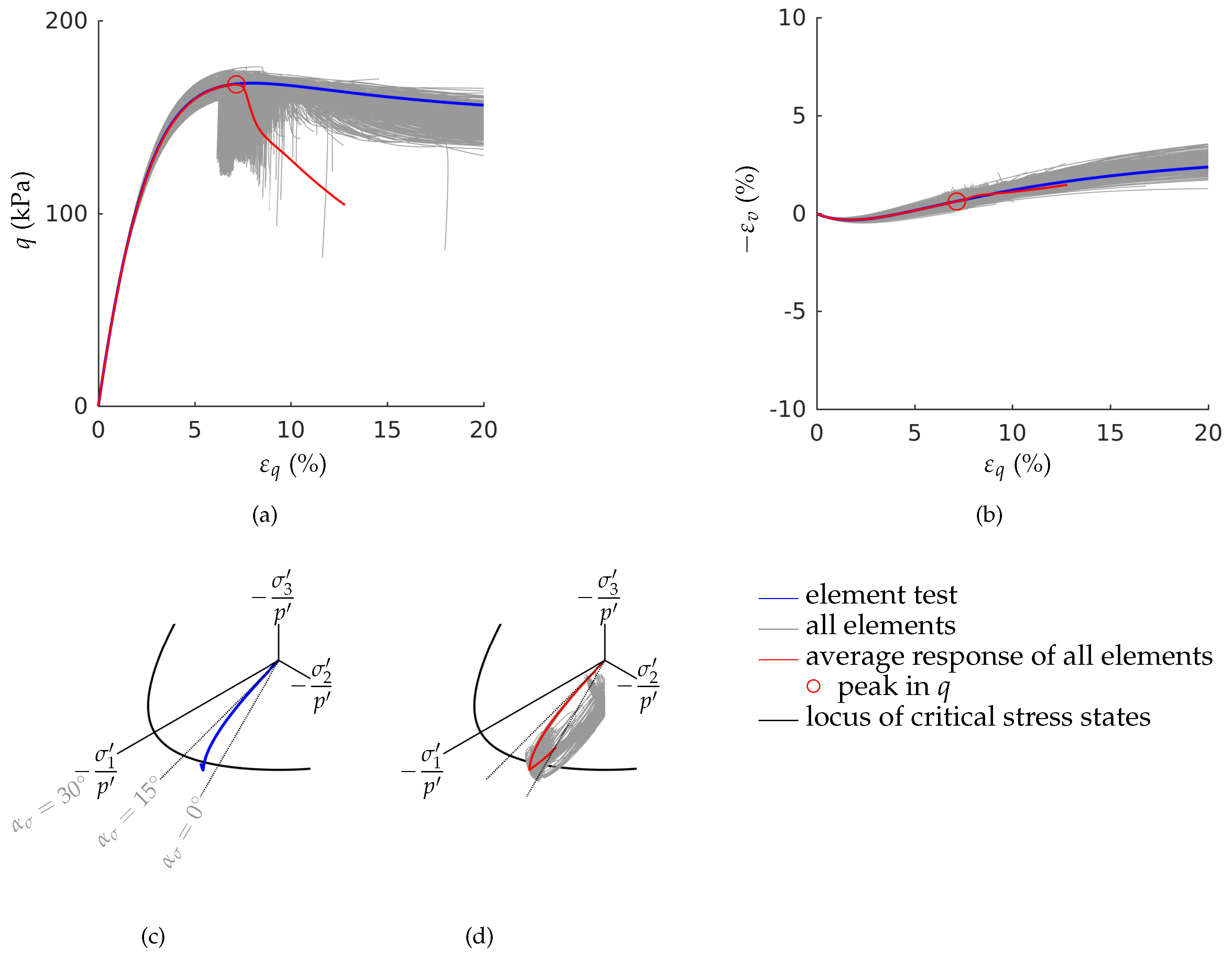
After the peak, the average response of the fine-meshed test shows a pronounced decrease in deviatoric stress compared to the single element test. The pronounced decrease results from the varying stress-strain curves in the individual elements, during softening, see Figure 14a, Figure 15a, Figure 16a and Figure 17a. The stress-strain curves that are close to the element test are inside the shear band. The stress-strain curves that are similar to unloading curves are outside the final shear band, see also Figure 4c and [22]. The average response shows a typical stress-strain curve of a biaxial test (e.g., [33]). Figure 14b, Figure 15b, Figure 16b and Figure 17b show the volumetric behaviour. Again the average response differs from the single element test.

3.2. Stress Paths in the Deviatoric Plane

In Figure 14c, Figure 15c, Figure 16c and Figure 17c the Lode angles according to Equation (4) ${\alpha }_{\sigma }=0^{\circ },{15}^{\circ }$ and ${30}^{\circ }$ are marked. At failure, stress paths of the average response of all elements (red line) as well as the stress paths of the element test in the simulations do not leave the range of $0^{\circ }<{\alpha }_{\sigma }<{15}^{\circ }$ for the OCR $=1.5$, 3 and 6. The experimental findings by Nakai [28], that the Lode angles under plane strain compression are within $0^{\circ }<{\alpha }_{\sigma }<{15}^{\circ }$ have been carried out on normally consolidated samples. The element test in Figure 14c reaches the locus of critical stress states of barodesy, whereas the average response reached a lower maximum mobilized friction angle which is inside the locus of critical stress states, see Figure 14d.

For the simulation with OCR $=54$, the increase of ${\sigma }_2^{\prime }$ is larger than in the simulations with lower overconsolidation ratios. The higher the OCR is, the higher is the dilatancy. By keeping the lateral expansion to zero (${\epsilon }_2=0$), higher stresses ${\sigma }_2^{\prime }$ develop for the OCR of 54 in Figure 17c,d than for OCR of $1.5$, 3 and 6, see Figure 14, Figure 15 and Figure 16c,d.

As expected, the highly overconsolidated samples in Figure 16 and Figure 17c,d include peak states which lie outside the locus of critical stress states; see also Figure 2b.

3.3. Inclination of the Final Shear Band

The shear band inclination is evaluated for the tests with $\psi >0^{\circ }$, that are the highly overconsolidated samples with OCR 6 and 54. The orientations of the shear bands are estimated according to Equations (6)–(8), see

Table 4. Inclination of final shear band.

OCR	$\mathit{\psi }$	${\mathit{\phi }}_{\mathit{m}}^{\mathbf{max}}={\mathit{\phi }}_{\mathit{FE}}^{\mathbf{max}}$	${\mathit{\theta }}_{\mathbf{R}}$	${\mathit{\theta }}_{\mathbf{MC}}$	${\mathit{\theta }}_{\mathbf{A}}$	$\mathit{\theta }$
6	${2.8}^{\circ }$	${29.4}^{\circ }$	${46.4}^{\circ }$	${59.7}^{\circ }$	${53.0}^{\circ }$	${49.5}^{\circ }$
54	${28.9}^{\circ }$	${35.4}^{\circ }$	${59.4}^{\circ }$	${62.7}^{\circ }$	${61.1}^{\circ }$	${60}^{\circ }$

. In the finite element simulations, the inclination of the shear band is evaluated just after the peak as soon as the inclination of the shear band is clearly visible, see Figure 8e and Figure 9d.

For an OCR of 6, the measured angle of $\theta ={49.5}^{\circ }$ lies between Roscoe’s solution (${\theta }_{\mathrm{R}}={49.4}^{\circ }$) and Arthur et al.’s predictions (${\theta }_{\mathrm{A}}={53.0}^{\circ }$), see Table 4. For the OCR of 54, the measured angle of $\theta ={60}^{\circ }$ is close to Roscoe’s solution with ${\theta }_{\mathrm{R}}={59.4}^{\circ }$, see Table 4.

4. Discussion and Conclusions

Soil is an inhomogeneous material as it consists of different grain sizes and grain shapes. A constant void ratio distribution over the entire sample is therefore not possible. Inhomogeneities in the samples density are also generated due to inhomogeneous sample mounting.

• Inhomogeneities in the samples density may be one cause for early shear bands development. Finite element simulations of fine-meshed biaxial test with the material model barodesy show this effect: In barodesy, the density is considered with the void ratio as state variable. A randomly distributed void ratio results in a scatter of dilatancy. Thus, pre-peak patterns of shear bands develop from the very beginning of the biaxial tests.
• The stress-strain behaviour of a biaxial test—in particular the post-peak behaviour—cannot be modelled with a single element test. In our simulations, the number of elements has been chosen in a way that the final shear band thickness is in the experimental confirmed range. A realistic estimation of the shear band thickness results in a realistic average response of the stress-strain behaviour, due to the pronounced localization.
• The stress paths in the deviatoric plane show reasonable results: The Lode angles of the stress paths for the OCRs 1.5, 3 and 6 are in the range of $0^{\circ }<{\alpha }_{\sigma }<{15}^{\circ }$, which is experimentally confirmed for plane strain failure.
• The maximum deviatoric stress in the element test is higher than the maximum deviatoric stress of the average response of the fine-meshed test. The lower the initial overconsolidation ratio is, the larger is the deviation in peak strength.
• The inclination of the final shear band is dependent on the overconsolidation ratio: The higher the overconsolidation ratio is, the larger is the inclination of the final shear band.

The investigations and results of this work can only be used for qualitative purposes. Future investigations should compare experiments with simulations. Other material models, e.g., hypoplastic models, which include the void ratio as a state variable are also suitable for the simulations.

References

- Herle, I. On basic features of constitutive models for geomaterials. J. Theor. Appl. Mech. 2008, 38, 61–80. [Google Scholar]
- Tejchman, J.; Herle, I.; Wehr, J. FE-studies on the influence of initial void ratio, pressure level and mean grain diameter on shear localization. Int. J. Numer. Anal. Methods Geomech. 1999, 23, 2045–2074. [Google Scholar] [CrossRef]
- Schneider-Muntau, B.; Chen, C.H.; Bathaeian, S.M.I. Simulation of shear bands with Soft PARticle Code (SPARC) and FE. GEM Int. J. Geomath. 2017, 8, 135–151. [Google Scholar] [CrossRef] [PubMed] [Green Version]
- Medicus, G.; Schneider-Muntau, B.; Kolymbas, D. Second-order work in barodesy. Acta Geotech. 2018. [Google Scholar] [CrossRef]
- Desrues, J.; Andò, E.; Bésuelle, P.; Viggiani, G.; Debove, L.; Charrier, P.; Toni, J.B. Localisation Precursors in Geomaterials? In Proceedings of the Bifurcation and Degradation of Geomaterials with Engineering Applications, IWBDG 2017, Limassol, Cyprus, 21–25 May 2017; Papamichos, E., Papanastasiou, P., Pasternak, E., Dyskin, A., Eds.; Springer International Publishing: Cham, Switzerland, 2017; pp. 3–10. [Google Scholar] [CrossRef]
- Medicus, G.; Fellin, W. An improved version of barodesy for clay. Acta Geotech. 2017, 12, 365–376. [Google Scholar] [CrossRef]
- Nübel, K. Experimental and Numerical Investigation of Shear Localization in Granular Material. Ph.D. Thesis, Veröffentlichungen des Institutes für Bodenmechanik und Felsmechanik der Universität Karlsruhe, Karlsruhe, Germany, 2002. [Google Scholar]
- Medicus, G.; Schneider-Muntau, B. Stress-dilatancy in barodesy. In Book of Extended Abstracts, 4th International Symposium on Computational Geomechanics, ComGeo IV, Assisi, Italy, 2–4 May 2018; International Centre for Computational Engineering: Rhodes, Greece; Swansea, UK, 2018; pp. 22–23. [Google Scholar]
- Von Wolffersdorff, P.A. A hypoplastic relation for granular materials with a predefined limit state surface. Mech. Cohesive-Frict. Mater. 1996, 1, 251–271. [Google Scholar] [CrossRef]
- Mašín, D. Clay hypoplasticity with explicitly defined asymptotic states. Acta Geotech. 2013, 8, 481–496. [Google Scholar] [CrossRef]
- Fellin, W.; Ostermann, A. The critical state behaviour of barodesy compared with the Matsuoka–Nakai failure criterion. Int. J. Numer. Anal. Methods Geomech. 2013, 37, 299–308. [Google Scholar] [CrossRef]
- Medicus, G.; Kolymbas, D.; Fellin, W. Proportional stress and strain paths in barodesy. Int. J. Numer. Anal. Methods Geomech. 2016, 40, 509–522. [Google Scholar] [CrossRef]
- Mašín, D. A hypoplastic constitutive model for clays. Int. J. Numer. Anal. Methods Geomech. 2005, 29, 311–336. [Google Scholar] [CrossRef]
- Butterfield, R. A natural compression law for soils (an advance on e-logp′). Géotechnique 1979, 29, 469–480. [Google Scholar] [CrossRef]
- Kolymbas, D. Sand as an archetypical natural solid. In Mechanics of Natural Solids; Kolymbas, D., Viggiani, G., Eds.; Springer: Berlin, Germany, 2009; pp. 1–26. [Google Scholar]
- Kolymbas, D. Introduction to barodesy. Géotechnique 2015, 65, 52–65. [Google Scholar] [CrossRef]
- Kolymbas, D.; Medicus, G. Genealogy of hypoplasticity and barodesy. Int. J. Numer. Anal. Methods Geomech. 2016, 40, 2532–2550. [Google Scholar] [CrossRef]
- Medicus, G. Barodesy and Its Application for Clay. Ph.D. Thesis, University of Innsbruck, Innsbruck, Austria, 2014. [Google Scholar]
- Medicus, G.; Fellin, W.; Schranz, F. Konzepte der Barodesie. Bautechnik 2018, 95, 620–638. [Google Scholar] [CrossRef]
- D’Ignazio, M.; Länsivaara, T. Shear bands in soft clays: Strain-softening behaviour in finite element method. Rakenteiden Mekaniikka 2015, 48, 83–98. [Google Scholar]
- Jostad, H.; Andresen, L.; Thakur, V. Calculation of shear band thickness in sensitive clays. In Proceedings of the 6th European Conference on Numerical Methods in Geotechnical Engineering, Graz, Austria, 6–8 September 2006; pp. 27–32. [Google Scholar]
- Pouragha, M.; Wan, R. Micromechanical study of instability in granular materials using μ-GM constitutive model. In Book of Extended Abstracts, 4th International Symposium on Computational Geomechanics, ComGeo IV, Assisi, Italy, 2–4 May 2018; International Centre for Computational Engineering: Rhodes, Greece; Swansea, UK, 2018; pp. 51–52. [Google Scholar]
- Gylland, A.S.; Jostad, H.P.; Nordal, S. Experimental study of strain localization in sensitive clays. Acta Geotech. 2014, 9, 227–240. [Google Scholar] [CrossRef]
- abaqus FEA 6.14, Simulia, Dassault Systèmes. 78140 Vélizy-Villacoublay, France, 2018. Available online: https://www.3ds.com/de/produkte-und-services/simulia/produkte/abaqus/ (accessed on 28 November 2018).
- Gudehus, G.; Amorosi, A.; Gens, A.; Herle, I.; Kolymbas, D.; Mašín, D.; Muir Wood, D.; Nova, R.; Niemunis, A.; Pastor, M.; et al. The soilmodels.info project. Int. J. Numer. Anal. Methods Geomech. 2008, 32, 1571–1572. [Google Scholar] [CrossRef]
- Bode, M.; Schranz, F.; Medicus, G.; Fellin, W. Vergleich unterschiedlicher Materialmodelle an einer Aushubsimulation. Geotechnik 2018, in press. [Google Scholar]
- Schneider-Muntau, B.; Medicus, G.; Fellin, W. Strength reduction method in Barodesy. Comput. Geotech. 2018, 95, 57–67. [Google Scholar] [CrossRef]
- Nakai, T. Modeling of soil behaviour based on tij concept. In Proceedings of the 13th ARCSMGE, Kolkata, India, 10 December 2007; Volume 2, pp. 69–89. [Google Scholar]
- Muir Wood, D. Soil Behaviour and Critical State Soil Mechanics; Cambridge University Press: Cambridge, UK, 1990. [Google Scholar]
- Alshibli, K.A.; Akbas, I.S. Strain localization in clay: Plane strain versus triaxial loading conditions. Geotech. Geol. Eng. 2006, 25, 45. [Google Scholar] [CrossRef]
- Roscoe, K.H. The Influence of Strains in Soil Mechanics. Géotechnique 1970, 20, 129–170. [Google Scholar] [CrossRef]
- Arthur, J.R.F.; Dunstan, T.; Al-Ani, Q.A.J.L.; Assadi, A. Plastic deformation and failure in granular media. Géotechnique 1977, 27, 53–74. [Google Scholar] [CrossRef]
- Desrues, J.; Zweschper, B.; Vermeer, P. Database for Tests on Hostun RF Sand; Technical Report; Institute for Geotechnical Engineering, University of Stuttgart: Stuttgart, Germany, 2000. [Google Scholar]
Figure 1.
Matsuoka-Nakai and Mohr-Coulomb failure surface are compared with barodesy in the deviatoric plane. Barodesy and Matsuoka-Nakai practically coincide [11]. Figure modified from [12].
Figure 2.
Barotropy in barodesy, figure modified from [19]: simulations with barodesy of CD triaxial tests with Weald clay with const. (a) mean stress - void ratio plot: highly overconsolidated samples (grayed area) dilate, normally and slightly overconsolidated samples contract under shearing. (b) mean stress - deviatoric stress plot: highly overconsolidated samples reach peak states which are higher than critical strength. (c) axial strain - stress ratio plot: highly overconsolidated samples reach higher stress ratios/mobilized friction angles than the critical friction angle.
Figure 3.
Pyknotropy in barodesy: simulations with barodesy of CD triaxial tests with Weald clay with const. (a) mean stress - void ratio plot: highly overconsolidated samples (grayed area) dilate, normally and slightly overconsolidated samples contract under shearing. (b) axial strain - deviatoric stress plot: the lower the initial void ratio is, the higher is peak strength. (c) axial strain - stress ratio plot: highly overconsolidated samples reach higher stress ratios/mobilized friction angles than the critical friction angle.
Figure 4.
(a) FE model (b) Final shear band at global deviatoric strain of , displayed as deviatoric strain, green: to red: (c) Stress-strain curves in-
A and outside B the shear band, single element test.
Figure 5.
For OCR follows the mean value , black line. The standard deviation is 0.005. The red lines mark the standard deviation, i.e., . (a) The initial void ratio is normally distributed over all 5000 elements. (b) shows the range in the e- plot with and .
Figure 6.
OCR = 1.5: Shear band development displayed with deviatoric strain in each element at different global deviatoric strain , peak in q is at . (a–c) show pre-peak pattern of shear bands, (d) peak and (e,f) post-peak pattern of shear bands.
Figure 7.
OCR = 3: Shear band development displayed with deviatoric strain in each element at different global deviatoric strain , peak in q is at . (a–c) show pre-peak pattern of shear bands, (d) peak and (e,f) post-peak pattern of shear bands.
Figure 8.
OCR = 6: Shear band development displayed with deviatoric strain in each element at different global deviatoric strain , peak in q is at . (a–c) show pre-peak pattern of shear bands, (d–f) post-peak pattern of shear bands.
Figure 9.
OCR = 54: Shear band development displayed with deviatoric strain in each element at different global deviatoric strain , peak in q is at . (a–c) show pre-peak pattern of shear bands, (d) peak and (e,f) post-peak pattern of shear bands.
Figure 10.
OCR : The global deviatoric strain marked with (a–f) corresponds to Figure 9a–f.
Figure 11.
OCR : The global deviatoric strain marked with (a–f) corresponds to Figure 7a–f.
Figure 12.
OCR : The global deviatoric strain marked with (a–f) corresponds to Figure 8a–f.
Figure 13.
OCR : The deviatoric strain marked with (a–f) corresponds to Figure 9a–f.
Figure 14.
OCR : (a) Deviatoric strain -deviatoric stress q plot; (b) Deviatoric strain -volumetric strain plot; (c,d) Stress paths for OCR in the deviatoric plane normalized with the mean effective stress .
Figure 15.
Figure 16.
Figure 17.