Hybrid Fixed-Point Fixed-Stress Splitting Method for Linear Poroelasticity

Abstract

Efficient and accurate poroelasticity models are critical in modeling geophysical problems such as oil exploration, gas-hydrate detection, and hydrogeology. We propose an efficient operator splitting method for Biot’s model of linear poroelasticity based on fixed-point iteration and constrained stress. In this method, we eliminate the constraint on time step via combining our fixed-point approach with a physics-based restraint between iterations. Three different cases are considered to demonstrate the stability and consistency of the method for constant and variable parameters. The results are validated against the results from the fully coupled approach. In case I, a single iteration is used for continuous coefficients. The relative error decreases with an increase in time. In case II, material coefficients are assumed to be linear. In the single iteration approach, the relative error grows significantly to 40% before rapidly decaying to zero. This is an artifact of the approximate solutions approaching the asymptotic solution. The error in the multiple iterations oscillates within ${10}^{-6}$ before decaying to the asymptotic solution. Nine iterations per time step are enough to achieve the relative error close to ${10}^{-7}$. In the last case, the hybrid method with multiple iterations requires approximately 16 iterations to make the relative error $5\times {10}^{-6}$.

1. Introduction

Linear poroelasticity is the relatively small deformations of fluid flow within a deformable porous medium. It can be found in diverse engineering fields such as reservoir engineering, biomechanics, environmental engineering [1,2,3,4], and earthquake engineering [5,6,7,8]. Stress analysis of bore-hole with poroelastic models can be found in [9,10]. In Biomechanics, such models are used to simulate tumor-induced stress levels in the brain [11,12]. In storage reservoirs, those models predict critical stresses [13,14] which compromise caprock integrity [15] and wellbore stability [16]. The accuracy of these stresses via prior or empirical approximations of material parameters and source term variability [17] depends on the representations of the elastic moduli and permeability factors [18]. However, a bias toward non-intrusive uncertainty quantification methods such as Collocation [19,20] and Monte Carlo [21,22,23] methods in many engineering applications [19,20,24,25,26,27], including poroelasticity [28,29]. These methods only require weighted sums of solutions to a problem at specific points in the random space [19]. However, intrusive methods are more efficient in achieving convergence per degree of freedom [17,30,31,32,33,34,35].

Poroelasticity is a coupled multiphysics problem where systems of partial differential equations describe the interactions between two or more field variables. Multiphysics problems differ from general mixed partial differential equation (PDE) formulations in that “neither domain can be solved separately from each other, and neither set of dependent variables can be explicitly eliminated” [36,37,38]. Such multiphysics problems often result in significant degrees of freedom and present computational challenges. Accurate and efficient poroelasticity models are critical in modeling such multiphase flows including geophysical issues. For example, oil exploration, gas-hydrate detection, and hydrogeology [39]. These models also play an essential role in other engineering applications such as induced seismicity, groundwater contamination, and material processing and mitigating associated concerns. High dimensionality and multiscale nature of these applications make the modeling a daunting task. Moreover, much progress has been made in mathematical modeling, numerical analysis, discretization techniques, and high-performance computing [40]. Stochastic models can address the high dimensional problem. However, it is challenging to carry out parametric or sensitivity analysis as those models are computationally expensive. On the other hand, advances in preconditioners for linear systems [17,41] and parallelization [42] methods can result in accurate results with far fewer total degrees of freedom compared to non-intrusive methods [30] and reduce the computational cost. The high fidelity multiscale simulations may be possible with advanced high-performance computers. Therefore, splitting methods are prevalent in modeling geomechanical problems due to their inherent ability to reuse existing fluid flow and solid mechanics solvers. The practical approach for poroelasticity is based solely on constraining the physics between iterations. The pioneering work of Kim [43] analyzed the stability and consistency of several splitting strategies, including the drained, undrained, fixed strain, and the fixed rate of stress. It was found that the fixed rate of stress approach yielded consistency even when a single iteration was used [44,45]. Rigorous stability and convergence analysis for those splitting methods can be found in [46]. We explored an alternative splitting strategy based on fixed point iteration [47,48]. We obtained a convergent splitting strategy based on fixed point iteration which did not depend on artificially constraining the physics between iterations. We found that our method was, however, conditionally stable upon choosing sufficiently large time steps. In the present work, we overcome the constraint on time step by combining our fixed-point approach with a physics-based restraint between iterations. The current approach differs from our previous work in that we constrain the stress directly, without considering the rate of strain. The hybrid method proposed in this work can be used to simulate complex geomechanics problems [49,50].

We propose a method which decomposes the multiscale poroelasticity equations [48,51,52] into a sequence of elliptic partial differential equations sufficiently general to capitalize on the ample algorithms available for multiscale elliptic PDE’s. This method is based on block operator splitting of poroelasticity equations based on fixed-point iterations. The resulting formulation contains a pair of continuous elliptic PDE subproblems with multiscale coefficients. The present method is unconditionally stable for various material parameters, grid spacings, and time step sizes. Besides, it is convergent even for linearly as well as randomly varying material parameters. The fixed-point iterative process is described in Section 2. The hybrid method is presented in Section 3. The convergence analysis of this method is presented in Section 4. In Section 5, we demonstrate that our approach has similar convergent properties to the undrained splitting method, but also converges in a single iteration in case of constant material parameters.

2. Fixed Stress Splitting

Consider a system modeling diffusion in an elastic medium where the inertial effects are negligible. This quasi-static assumption arises naturally in the classical Biot model of consideration for a linearly elastic and porous solid which is saturated by a slightly compressible viscous fluid. The fluid pressure is denoted by p and the displacement of the structure by u. The equations governing the poro-elastic system [53] for a homogeneous and isotropic medium are

$$-(\lambda +\mu )\nabla (\nabla .u)-\mu {\nabla }^{2}u+\alpha \nabla p=f,$$

(1)

$$\frac{\partial }{\partial t}(c_{0}p+\alpha \nabla .u)-\nabla .k(\nabla p)=g.$$

(2)

where, $\lambda$, $\mu$, $\alpha$, $c_0$, and k are material parameters, f is the body force, and g is the source term. The flow Equation (2) can be discretized in time (t) and space (x) with the forward finite difference scheme as

$$c_0\frac{p^{t+1}-p^t}{\Delta t}+\alpha \frac{{ϵ}_v^{t+1}-{ϵ}_v^t}{\Delta t}-\frac{d}{dx}(k(x)\frac{d{p}^{t+1}}{dx})=g,$$

(3)

where ${ϵ}_v^t\equiv \nabla ·u^t$ is the volumetric strain. The superscript t and $t+1$ represents quantities at time t and $t+1$, respectively. The traditional fixed rate of stress operator splitting strategy [44] for poroelasticity is a well-studied method with good convergence properties. It is based on imposing a constraint upon the volumetric stress in the flow equation. However, it is more appropriately interpreted not as fixed stress, but as fixed rate of stress since it constrains the variation in the time derivative of the volumetric stress (${\sigma }_v$) as

$$\delta {\dot{\sigma }}_v=0.$$

(4)

The discrete form of Equation (4) is

$$\frac{{\sigma }_v^{t+1}-{\sigma }_v^t}{\Delta t}-\frac{{\sigma }_v^t-{\sigma }_v^{t-1}}{\Delta t}=0,$$

(5)

To convert Equation (5) in terms of the primary variable u, we use the following relation between volumetric stress (${\sigma }_v$), volumetric strain (${ϵ}_v$), and pore pressure (p)

$${\sigma }_v-{\sigma }_{v,0}=K_{dr}(x){ϵ}_v-\alpha \left(p-p_0\right),$$

(6)

where $K_{dr}$ is unit bulk modulus constant. The derivative of Equation (6) with respect to t is

$$\frac{d{\sigma }_v}{dt}=K_{dr}(x)\frac{d{ϵ}_v}{dt}-\alpha \frac{dp}{dt}.$$

(7)

The forward and backward finite difference approximations of Equation (7) with respect to time step t are

$$\frac{{\sigma }_v^{t+1}-{\sigma }_v^t}{\Delta t}=K_{dr}(x)\frac{{ϵ}_v^{t+1}-{ϵ}_v^t}{\Delta t}-\alpha \frac{p^{t+1}-p^t}{\Delta t}$$

(8)

and

$$\frac{{\sigma }_v^t-{\sigma }_v^{t-1}}{\Delta t}=K_{dr}(x)\frac{{ϵ}_v^t-{ϵ}_v^{t+1}}{\Delta t}-\alpha \frac{p^t-p^{t+1}}{\Delta t},$$

(9)

respectively. By substituting these discrete derivatives into Equaton (5) and solving for ${ϵ}_v^{t+1}$, we get

$${ϵ}_v^{t+1}=2{ϵ}_v^t-{ϵ}_v^{t-1}+\frac{\alpha }{K_{dr}(x)}\left(p^{t+1}-2p^t+p^{t-1}\right).$$

(10)

By substituting Equation (10) into Equation (3), we eliminate the flow equation’s dependence on ${ϵ}_v^{t+1}$ and can solve for $p^{t+1}$ alone. Note that Equation (10) suggests that this splitting strategy requires only a single solve of the flow equation and requires information at time-steps t and $t-1$.

3. Hybrid Method

Based on our fixed stress splitting strategy, we propose a simple method to accelerate our iterative splitting strategy. First, we recall our semi-discrete Equation (3) and consider a sequence of approximations n within the time-step $t+1$ by replacing the unknown variables ${\sigma }_v^{t+1}$ and $p^{t+1}$ with ${\sigma }_v^{t+1,n+1}$ and $p^{t+1,n+1}$, respectively. This applies to both the fluid and solid equations, but we modify the fluid equation using a slightly different method. Substituting the $n+1$ iterates into Equation (3), we get

$$\begin{array}{c}\hfill \left(c_0+\frac{K_{dr}(x)}{\alpha }\right)\frac{p^{t+1,n+1}-p^t}{\Delta t}+\left(\frac{\alpha }{K_{dr}(x)}\right)\frac{{ϵ}_v^{t+1,n+1}-{ϵ}_v^t}{\Delta t}-\frac{d}{dx}\left(k(x)\frac{d{p}^{t+1,n+1}}{dx}\right)=g.\end{array}$$

(11)

Note that the iterations occur only over the unknowns $p^{t+1}$ and ${ϵ}_v^{t+1}$ and that dependence of Equation (11) on ${ϵ}_v^{t+1,n+1}$ implies dependence on $\nabla ·u^{t+1,n+1}$ as well. To remove this dependence, we impose a slightly different constraint from the traditional fixed stress splitting. Instead of constraining the variation in the rate of volumetric stress $\delta \dot{{\sigma }_v}=0$, we constrain the variation in volumetric stress at the time level $t+1$ over the iterations n and $n+1$. This constraint is written as

$$\delta {\dot{\sigma }}_v^{t+1,n}=0$$

or equivalently

$${\sigma }_v^{t+1,n+1}-{\sigma }_v^{t+1,n}=0.$$

(12)

Again, we use the relation between volumetric stress, volumetric strain, and pore pressure in Equation (6). By reformulating this relation in terms of iterations n and $n+1$ and substituting that in Equation (12), we obtain

$${ϵ}_v^{t+1,n+1}={ϵ}_v^{t+1,n}+\frac{\alpha }{K_{dr}(x)}\left(p^{t+1,n+1}-p^{t+1,n}\right).$$

(13)

Substituting Equation (13) into Equation (11), we eliminate the flow equation’s dependence on $u^{t+1,n+1}$ and enable a solution in terms of pressure terms $p^{t+1,n+1}$ only. Note that this new approach differs from both the traditional fixed-stress splitting and the fixed-point iteration described earlier and is a hybrid of both approaches. This approach is also like the undrained splitting method, as described by Mikelić and Wheeler in [46]. The primary difference is that our method removes the flow equation dependence on ${ϵ}_v$ instead of removing solid equation dependence on p.

We utilize the fixed-point iteration to set up a fully implicit sequence of approximations within the time step t. We also utilize the volumetric stress equation to remove the dependencies on the volumetric strain in the current iteration. Unlike the traditional fixed-stress splitting, we hold the volumetric stress constant between iterations instead of its time derivative. In doing so, the new approximation $p^{t+1,n+1}$ in our hybrid approach does not require the information from two previous time steps $p^t$ and $p^{t-1}$ as seen in the traditional fixed-stress splitting approach. Instead, it utilizes only information from the previous time step $p^t$ and the previous iteration $p^{t+1,n}$ to determine the variable in the next iteration $p^{t+1,n+1}$.

4. Convergence

Instead of analyzing the eigenvalues of the stationary matrix as in [47], we establish stability by von Neumann analysis in the case of constant coefficients $K_{dr}(x)\equiv K_{dr}$ and $k(x)\equiv k$. To achieve this, we first reinterpret the hybrid fixed point iteration method as a single-pass splitting method. Consider the fixed-point iteration equations with no source terms (g)

$$\begin{array}{c}\hfill -K_{dr}\frac{d}{dx}\left(\frac{d{u}^{t+1,n+1}}{dx}\right)+\alpha \frac{d{p}^{t+1,n+1}}{dx}=0,\end{array}$$

(14)

$$\begin{array}{c}\hfill \left(c_0+\frac{K_{dr}}{\alpha }\right)\frac{p^{t+1,n+1}-p^t}{\Delta t}+\left(\frac{\alpha }{K_{dr}}\right)\frac{{ϵ}_v^{t+1,n+1}-{ϵ}_v^t}{\Delta t}-k\frac{d}{dx}\left(\frac{d{p}^{t+1,n+1}}{dx}\right)=0.\end{array}$$

(15)

Substituting Equation (13) into Equation (15), the flow equation yields

$$\begin{array}{c}\hfill \frac{c_0+\frac{1}{\tau }+{\tau }^2}{\Delta t}{p}^{t+1,n+1}+\frac{c_0+\tau }{\Delta t}{p}^t-\frac{{\tau }^2}{\Delta t}{p}^{t+1,n}+\frac{\tau }{\Delta t}{ϵ}_v^{t+1,n}-\frac{\tau }{\Delta t}{ϵ}_v^t-k\frac{d}{dx}\left(\frac{d{p}^{t+1,n+1}}{dx}\right)=0,\end{array}$$

(16)

where $\tau \equiv \frac{\alpha }{K_{dr}}$. If we invoke only a single iteration in Equation (15), then we can write Equation (16) as

$$\begin{array}{c}\hfill \frac{c_0+\frac{1}{\tau }+{\tau }^2}{\Delta t}{p}^{t+1}+\frac{c_0+\tau }{\Delta t}{p}^t-\frac{{\tau }^2}{\Delta t}{p}^{*}+\frac{\tau }{\Delta t}{ϵ}_v^{*}-\frac{\tau }{\Delta t}{ϵ}_v^t-k\frac{d}{dx}\left(\frac{d{p}^{t+1}}{dx}\right)=0,\end{array}$$

(17)

where ${ϵ}_v^{*}$ and $p^{*}$ are predicted values at the time step $t+1$. Naturally, if $\Delta t$ is sufficiently small, then we expect the predicted values are close to the values at the previous time-step t. Thus, we choose $p^{*}=p^t$ and ${ϵ}_v^{*}={ϵ}_v^t$. Substituting these predictors into Equation (17), we completely decouple the flow equation from its dependence on displacement u by canceling the ${ϵ}_v$ terms. Hence, (17) becomes

$$\frac{c_0+\frac{1}{\tau }+{\tau }^2}{\Delta t}\left(p^{t+1}-p^t\right)-k\frac{d}{dx}\left(\frac{d{p}^{t+1}}{dx}\right)=0.$$

(18)

We can write Equation (15) as

$$-K_{dr}\frac{d}{dx}\left(\frac{d{u}^{t+1}}{dx}\right)+\alpha \frac{d{p}^{t+1}}{dx}=0.$$

(19)

Now, we discretize this system of equations on an equispaced, staggered finite volume cell grid and obtain

$$\begin{array}{c}\hfill -\frac{K_{dr}}{\Delta x}\left(u_{j-\frac{3}{2}}^{t+1}-2u_{j-\frac{1}{2}}^{t+1}+u_{j+\frac{1}{2}}^{t+1}\right)+\alpha \left(p_j^{t+1}-p_{j-1}^{t+1}\right)=0\end{array}$$

(20)

$$\begin{array}{c}\hfill \frac{\Delta x\left(c_0+\frac{1}{\tau }+{\tau }^2\right)}{\Delta t}\left(p_j^{t+1}-p_j^t\right)-\frac{k}{\Delta x}\left(p_{j-1}^{t+1}-2p_j^{t+1}+p_{j+1}^{t+1}\right)=0\end{array}$$

(21)

In a similar manner to [43], we assess the stability of the time stepping scheme in the context of Von Neumann analysis by considering a characteristic solution of the form $p_j^t={\gamma }^n{e}^{ij\theta }\widehat{P}$ and $u_j^t={\gamma }^n{e}^{ij\theta }\widehat{U}$, with $\theta \in [-\pi ,\pi ]$ and amplification factor $\gamma$. Substituting these expressions in Equation (20) and utilizing half angle and complex exponential identities, we obtain

$$\begin{array}{c}\hfill \left[\begin{array}{cc}\frac{1}{\tau \Delta x}\left(1-cos\theta \right)& \alpha isin\left(\frac{\theta }{2}\right)\\ 0& \left(b_1\left(\gamma -1\right)+b_2\gamma \right)\end{array}\right]\left[\begin{array}{c}\widehat{U}\\ \widehat{P}\end{array}\right]=\left[\begin{array}{c}0\\ 0\end{array}\right],\end{array}$$

(22)

where $b_1=\Delta x\left(c_0+\frac{1}{\tau }+{\tau }^2\right)$ and $b_2=\frac{2k\Delta t}{\Delta x}\left(1-cos\theta \right)$. We equate the determinant of the matrix in Equation (22) to zero and obtain the characteristic polynomial in terms of $\gamma$ as

$$\frac{1}{\Delta x}\left(1-cos\theta \right)·\left((b_1+b_2)\gamma -b_1\right)=0.$$

(23)

Note that Equation (23) is automatically satisfied for $(1-cos\theta )=0$. Thus, to show stability we need to demonstrate that the roots of Equation (23) have magnitude less than 1 in the case when $(1-cos\theta )\ne 0$. If we assume $(1-cos\theta )\ne 0$, then the root is

$$\gamma =\frac{b_1}{b_1+b_2}=\frac{\left(c_0+\frac{1}{\tau }+{\tau }^2\right)}{\left(c_0+\frac{1}{\tau }+{\tau }^2\right)+\frac{2k\Delta t}{\Delta x^2}(1-cos\theta )}.$$

(24)

Since $c_0,\tau ,\Delta t$, and $\Delta x$ are positive and $(1-cos\theta )>0$ for all $\theta$, the numerator is clearly smaller than the denominator in magnitude. Thus, $\left|\gamma \right|<1$ and our method is stable.

Stability alone does not necessarily result in convergence. By Lax equivalence theorem, we also need to show consistency. That is, the local truncation error $L(\Delta t,\Delta x)\to 0$ as $(\Delta t,\Delta x)\to (0,0)$ must hold true. By Taylor series expansions of the finite difference scheme, it is clear that Equation (18) has local truncation error $O(\Delta t+\Delta x^2)$. If we consider the pressure term in Equation (20) as a source term, then the displacement terms clearly retain a local truncation error $O(\Delta x)$. Since the local truncation errors in both equations are linear combinations of $\Delta t$ and $\Delta x$, their limits converge to 0 as $(\Delta t,\Delta x)\to (0,0)$.

5. Numerical Experiments

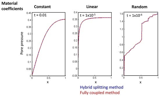
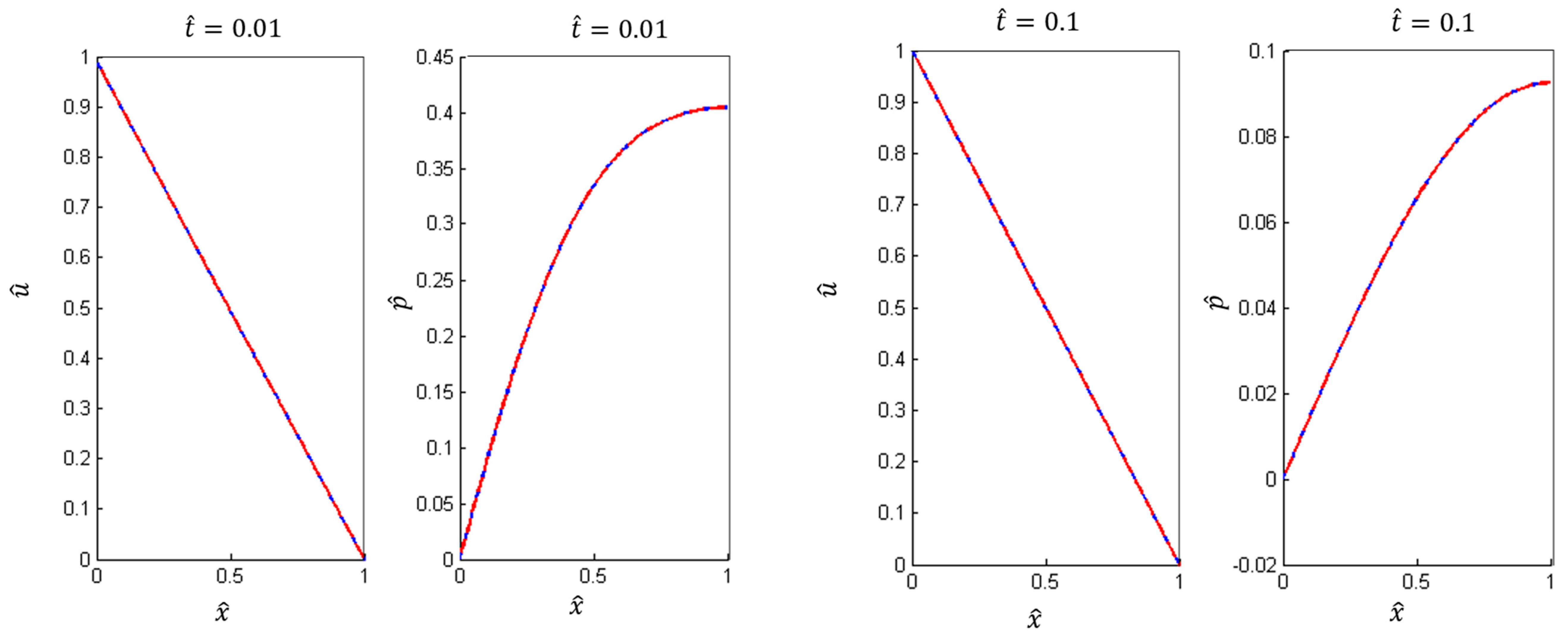
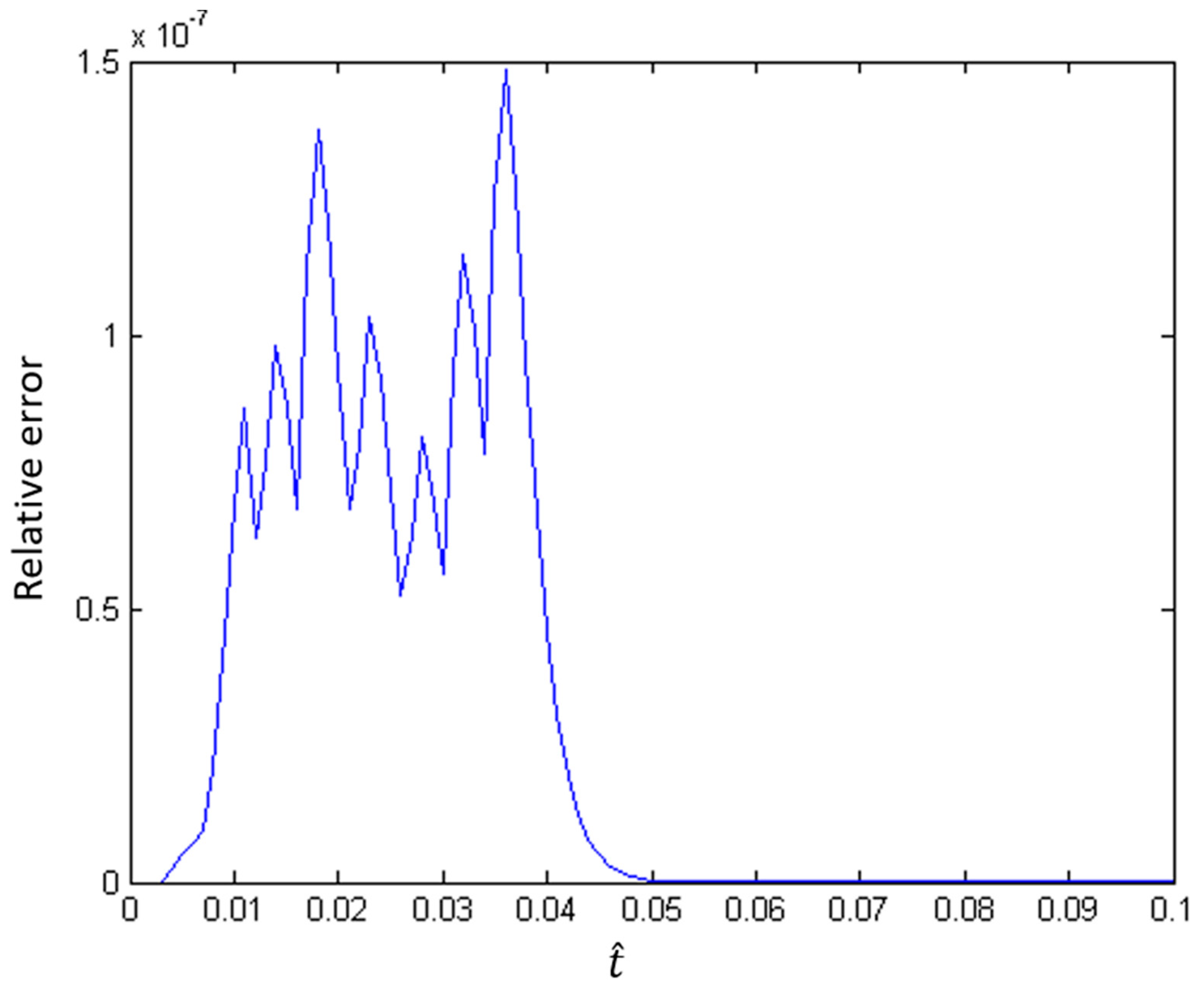
We have demonstrated the convergence of the hybrid splitting method in the case of constant material parameters with a single iteration. However, this analysis does not necessarily hold for the general example of variable coefficient parameters. In the present study, we demonstrate that this method does, indeed, converge over a wide range of cases when multiple iterations are allowed. The technique is particularly useful in the case of different material parameters.

We considered three different cases. In Case I, we have demonstrated the convergence of the hybrid splitting method in the case of constant material parameters with a single iteration. However, this analysis does not necessarily hold for the general example of variable coefficient parameters. We demonstrate that this method does, indeed, converge over a wide range of cases when multiple iterations are allowed. The splitting method is particularly useful in case of different material parameters. Case II explores the convergence of the hybrid splitting method with bulk modulus and mobility parameters expressed as linear functions of the form $f(x)=mx+b$. The third/final case illustrates the application of the hybrid method for randomly distributed $K_{dr}$ and k in the range $[1,1000]$ for both parameters.

In all the three cases, we chose a staggered spatial discretization consisting of $N=1000$ intervals in both u and v, yielding a total of $2N+2$ nodes on the unit interval $\Omega =[0,1]$. We applied the standard boundary conditions for the Terzaghi problem (See Figure 1). On the left boundary, pressure ($p_L=0$) and traction ($T_L=-1$) is specified. On the right boundary, displacement ($u_R=0$) and flux ($f_R=0$) is applied. If $p_L=u_R=f_R=0$ and $\lambda$, $\mu$, $\alpha$, $c_0$ and k are constant, then Equations (1) and (2) are equivalent to the classic Terzaghi Problem where a constant (compressive) load $T_L$ is suddenly applied on the top ($x=0$) of a column of fluid-saturated porous medium over a finite length. The load is induced by a permeable plunger or piston such that fluid drains through the top boundary as shown in Figure 1. Due to draining, the medium at the top boundary is also subject to zero excess pore pressure conditions. The Dirichlet and Neumann conditions at $x=1$ model the situation where the bottom wall is both rigid and impermeable, respectively. The medium is constrained in the transversal directions by a rigid container such that it is subject only to uniaxial strain. The initial condition captures the fact that there is no increment in fluid content upon initial loading. Next, we assume the lame parameters $\lambda$, $\mu$, and permeability k in Equations (1) and (2) vary in space but not in time. We further assume that these variable material parameters are highly heterogeneous, but not necessarily periodic.

To verify convergence, we compare the hybrid splitting solution to the numerical solution of the fully coupled poroelasticity equations. For both the hybrid splitting and fully combined solutions, the initial condition is obtained by imposing the increment in fluid content as zero. To simplify our analysis, we nondimensionalize the governing equations by introducing new spatial, temporal, and state variables. We follow an analogous approach [54] for nondimensionalizing the equations with the domain length L and traction boundary condition $T_L$. The non-dimensional space ($\widehat{x}$) $=\frac{x}{L}$, time ($\widehat{t}$) $=\frac{\nu kt}{L^2}$, pressure ($\widehat{p}$) $=\frac{p}{T_L}$, and displacement ($\widehat{u}$) $=\frac{\nu u}{T_{L}L}$. Where, $\nu =\lambda +2\mu$. Substituting these non-dimensional variables into the equations results a parameter associated with $\nabla p$, $\beta$, is $c_0\nu$. In the present study, the nondimensional domain, $\Omega$, is [0,1]. $\alpha \in [0,1]$ characterizes the strength of the coupling between the flow and deformation equations. If $\alpha =0$, then the equations for fluid and solid are completely decoupled from each other. In contrast, the case with $\alpha =1$ characterizes the strongest fluid-solid interactions.

6. Results

6.1. Case I

As Figure 2 illustrates, the fully coupled and hybrid splitting solutions are virtually indistinguishable from each other when only a single iteration is applied to the constant coefficient case. A good agreement in both pressures and displacements from the two solutions across all time steps can be seen in the figure. Figure 3 shows the relative $L^{\infty }$ norm error. Despite the small initial relative error, we observe that the error increases at the beginning of the computations and decreasing as $t\to \infty$. It is anticipated that any initial error should be monotonically amplified with successive time steps. We attribute the decrease in error to the convergence of both the hybrid and fully coupled solutions to an asymptotic state for the Terzaghi problem with no source terms.

6.2. Case II

We chose $f(x)=1000x+1$ ($m=1000$) as the variable material coefficient for $K_{dr}$ and k for all simulations. To capture the salient behavior of the partial differential equations, we chose a smaller time step $\Delta t=0.0001$ than that of Case I. Figure 4 and Figure 5 illustrate a stark contrast in the case of variable material coefficients. The error between the hybrid and fully coupled solutions is significantly large in magnitude. The visible difference between the solutions can be seen in Figure 4. In multiple time steps, nine iterations per time step are enough to achieve relative error close to ${10}^{-7}$. The solution converges with sufficiently small error to render the solutions visually indistinguishable.

The error plots (Figure 6 and Figure 7) confirm the stark difference in relative error between a single and multiple iterations of the hybrid method. In the only iteration approach, the error grows significantly to $40\%$ relative error before rapidly decaying to zero. Again, this is an artifact of the approximate solutions approaching the asymptotic solution, rather than convergence between the hybrid and fully coupled solutions. The error in the multiple iterations oscillates within ${10}^{-6}$ error before decaying to the asymptotic solution. Both approaches appear to converge to the asymptotic solution, but the evolution in time is more easily captured with multiple iterations for linear material coefficients.

6.3. Case III

For the linear case, we observe that convergence is not guaranteed for a single iteration when the real coefficients $K_{dr}$ and k vary in space. Thus, for case III, we only consider the hybrid method with multiple iterations. We note that, for this case, approximately sixteen iterations are required to achieve the relative error close to $5\times {10}^{-6}$. Figure 8 illustrates that the hybrid method again converges to the desired accuracy when multiple iterations are utilized. The error is well controlled overall time steps. Still, we observe that the error initially increases, but then stabilizes and decreases beyond this point. Though not illustrated in Figure 9, further analysis of the error reveals a steady decay of the error to zero as $t\to \infty$. Again, this phenomenon is a result of the rapid convergence of the numerical solution to its asymptotic state, rather than a property of the hybrid splitting method itself.

7. Conclusions

We developed an innovative operator splitting method for poroelasticity which combines the fixed-point iteration approach with the physics-based fixed-stress splitting. In this method, the constraint on time step is eliminated, and it accelerates the fixed stress method. We considered three different cases. In case I, we verify the convergence of the single iteration hybrid method for constant unit bulk modulus and constant unit mobility. In case II, we study the convergence of the process for linear bulk modulus and mobility parameters. Case III presents the application of the hybrid method for randomly distributed bulk modulus and mobility constants. In all the three cases, we chose a staggered spatial discretization consisting of $N=1000$ intervals in both x and y directions, yielding a total of $2N+2$ nodes on the unit interval $\Omega =[0,1]$. We compared results from the hybrid splitting method with the solution from fully coupled poroelasticity equations.

In case I, the relative error with the single iteration method decreases with an increase in time. In case II, the relative error with an only iteration approach grows significantly to 40% before rapidly decaying to zero. This is an artifact of the approximate solutions approaching the asymptotic solution. The error with multiple iterations oscillates within ${10}^{-6}$ before declining to the asymptotic solution. Nine iterations per time step are enough to achieve the relative error close to ${10}^{-7}$. In case III, the hybrid method with multiple iterations requires 16 iterations to make the relative error close to $5\times {10}^{-6}$. Therefore, numerous iterations per time step are needed if the real coefficients are not constant. We observed that both methods converge in few iterations and the results from these two methods are in good agreement. However, this approach is considerably difficult to implement in higher dimensions for arbitrary assignments of the Neumann and Dirichlet conditions, much less for arbitrary domain geometries. In contrast, the Dirichlet/Neumann center strategies are readily amenable to higher dimensions. More importantly, both approaches are needed to enable coupling between the flow and deformation problems.

References

1. Hudson, J.; Stephansson, O.; Andersson, J.; Tsang, C.F.; Jing, L. Coupled T-H-M issues relating to radioactive waste repository design and performance. Int. J. Rock Mech. Min. Sci. 2001, 38, 143–161. [Google Scholar] [CrossRef]
2. Descamps, F.; Descamps, F. Engineering Challenges in the Geological Disposal of Radioactive Waste and Carbon Dioxide. In Geological Disposal of Carbon Dioxide and Radioactive Waste: A Comparative Assessment; Springer: Berlin, Germany, 2011; pp. 185–213. [Google Scholar]
3. Shukla, R.; Ranjith, P.; Choi, S.; Haque, A. Study of caprock integrity in geosequestration of carbon dioxide. Int. J. Geomech. 2010, 11, 294–301. [Google Scholar] [CrossRef]
4. Mazzoldi, A.; Rinaldi, A.P.; Borgia, A.; Rutqvist, J. Induced seismicity within geological carbon sequestration projects: Maximum earthquake magnitude and leakage potential from undetected faults. Int. J. Greenh. Gas Control 2012, 10, 434–442. [Google Scholar] [CrossRef]
5. Harris, R.A. Introduction to Special Section: Stress Triggers, Stress Shadows, and Implications for Seismic Hazard. J. Geophys. Res. Solid Earth 1998, 103, 24347–24358. [Google Scholar] [CrossRef] [Green Version]
6. Jing, L. A review of techniques, advances and outstanding issues in numerical modeling for rock mechanics and rock engineering. Int. J. Rock Mech. Min. Sci. 2003, 40, 283–353. [Google Scholar] [CrossRef]
7. Baig, A.; Urbancic, T.; Viegas, G.; Karimi, S. Can small events (M < 0) observed during hydraulic fracture stimulations initiate large events (M > 0)? Lead. Edge 2012, 31, 1470–1474. [Google Scholar]
8. Davies, R.; Foulger, G.; Bindley, A.; Styles, P. Induced Seismicity and Hydraulic Fracturing for the Recovery of Hydrocarbons. Mar. Pet. Geol. 2013, 171–185. [Google Scholar] [CrossRef]
9. Detournay, E.; Cheng, A.D. Poroelastic response of a borehole in a non-hydrostatic stress field. Int. J. Rock Mech. Min. Sci. Geomech. Abstr. 1988, 25, 171–182. [Google Scholar] [CrossRef]
10. Rajapakse, R.K.N.D. Stress Analysis of Borehole in Poroelastic Medium. J. Eng. Mech. 1993, 119, 1205–1227. [Google Scholar] [CrossRef]
11. Roose, T.; Netti, P.A.; Munn, L.L.; Boucher, Y.; Jain, R.K. Solid stress generated by spheroid growth estimated using a linear poroelasticity model. Microvasc. Res. 2003, 66, 204–212. [Google Scholar] [CrossRef]
12. Byrne, H.; Preziosi, L. Modelling solid tumor growth using the theory of mixtures. Math. Med. Biol. J. IMA 2003, 20, 341–366. [Google Scholar] [CrossRef]
13. Zoback, M.D.; Gorelick, S.M. Earthquake triggering and large-scale geologic storage of carbon dioxide. Proc. Natl. Acad. Sci. USA 2012, 109, 10164–10168. [Google Scholar] [CrossRef] [PubMed] [Green Version]
14. Rutqvist, J.; Liu, H.H.; Vasco, D.W.; Pan, L.; Kappler, K.; Majer, E. Coupled non-isothermal, multiphase fluid flow, and geomechanical modeling of ground surface deformations and potential for induced micro-seismicity at the In Salah CO2 storage operation. Energy Procedia 2011, 4, 3542–3549. [Google Scholar] [CrossRef]
15. Oldenburg, C.M. The risk of induced seismicity: Is cap-rock integrity on shaky ground? Greenh. Gases Sci. Technol. 2012, 2, 217–218. [Google Scholar] [CrossRef]
16. Moos, D.; Peska, P.; Finkbeiner, T.; Zoback, M. Comprehensive wellbore stability analysis utilizing quantitative risk assessment. J. Pet. Sci. Eng. 2003, 38, 97–109. [Google Scholar] [CrossRef]
17. Le Maitre, O.O.P.; Knio, O.M. Spectral Methods for Uncertainty Quantification: With Applications to Computational Fluid Dynamics; Springer: Berlin, Germany, 2010. [Google Scholar]
18. Govindarajan, S. Geomechanical Characterization of Reservoir & Cap Rocks for CO2 Sequestration. Master’s Thesis, Missouri University of Science and Technology, Rolla, MO, USA, 2012. [Google Scholar]
19. Xiu, D. Numerical Methods for Stochastic Computations: A Spectral Method Approach; Princeton University Press: Princeton, NJ, USA, 2010. [Google Scholar]
20. Foo, J.; Karniadakis, G.E. Multi-element probabilistic collocation method in high dimensions. J. Comput. Phys. 2010, 229, 1536–1557. [Google Scholar] [CrossRef]
21. Wang, S.J.; Hsu, K.C. The application of the first-order second-moment method to analyze poroelastic problems in heterogeneous porous media. J. Hydrol. 2009, 369, 209–221. [Google Scholar] [CrossRef]
22. Mendes, M.A.; Murad, M.A.; Pereira, F. A new computational strategy for solving two-phase flow in strongly heterogeneous poroelastic media of evolving scales. Int. J. Numer. Anal. Methods Geomech. 2012, 36, 1683–1716. [Google Scholar] [CrossRef]
23. Farnoosh, R.; Ebrahimi, M. Monte Carlo method for solving Fredholm integral equations of the second kind. Appl. Math. Comput. 2008, 195, 309–315. [Google Scholar] [CrossRef]
24. Venkovic, N.; Sorelli, L.; Sudret, B.; Yalamas, T.; Gagné, R. Uncertainty propagation of a multiscale poromechanics-hydration model for poroelastic properties of cement paste at early-age. Probab. Eng. Mech. 2013, 32, 5–20. [Google Scholar] [CrossRef] [Green Version]
25. Azevedo, J.S.; Murad, M.A.; Borges, M.R.; Oliveira, S.P. A space-time multiscale method for computing statistical moments in strongly heterogeneous poroelastic media of evolving scales. Int. J. Numer. Methods Eng. 2012, 90, 671–706. [Google Scholar] [CrossRef]
26. Frias, D.G.; Murad, M.A.; Pereira, F. Stochastic computational modeling of highly heterogeneous poroelastic media with long-range correlations. Int. J. Numer. Anal. Methods Geomech. 2004, 28, 1–32. [Google Scholar] [CrossRef]
27. Menéndez, C.; Nieto, P.; Ortega, F.; Bello, A. Non-linear analysis of the consolidation of an elastic saturated soil with incompressible fluid and variable permeability by {FEM}. Appl. Math. Comput. 2010, 216, 458–476. [Google Scholar] [CrossRef]
28. El-Maghraby, N.M.; Yossef, H.M. State space approach to generalized thermoelastic problem with thermomechanical shock. Appl. Math. Comput. 2004, 156, 577–586. [Google Scholar] [CrossRef]
29. Zhang, W.; Li, X. Analytic solution of poromechanical problems in a hollow axisymmetric domain. Appl. Math. Comput. 1998, 97, 209–221. [Google Scholar]
30. Bäck, J.; Nobile, F.; Tamellini, L.; Tempone, R. Stochastic spectral Galerkin and collocation methods for PDEs with random coefficients: A numerical comparison. In Spectral and High Order Methods for Partial Differential Equations; Springer: Berlin, Germany, 2011; pp. 43–62. [Google Scholar]
31. Xiu, D.; Karniadakis, G.E. The Wiener–Askey polynomial chaos for stochastic differential equations. SIAM J. Sci. Comput. 2002, 24, 619–644. [Google Scholar] [CrossRef]
32. Najm, H.N. Uncertainty quantification and polynomial chaos techniques in computational fluid dynamics. Ann. Rev. Fluid Mech. 2009, 41, 35–52. [Google Scholar] [CrossRef]
33. Xiu, D.; Lucor, D.; Su, C.; Karniadakis, G.E. Stochastic modeling of flow-structure interactions using generalized polynomial chaos. J. Fluid Eng. 2002, 124, 51–59. [Google Scholar] [CrossRef]
34. Chen, X.; Ng, B.; Sun, Y.; Tong, C. A flexible uncertainty quantification method for linearly coupled multi-physics systems. J. Comput. Phys. 2013, 248, 383–401. [Google Scholar] [CrossRef]
35. Chen, Y.; Luo, Y.; Feng, M. Analysis of a discontinuous Galerkin method for the Biot’s consolidation problem. Appl. Math. Comput. 2013, 219, 9043–9056. [Google Scholar] [CrossRef]
36. Zienkiewicz, O. Coupled Problems and Their Numerical Solution. In Numerical Methods in Coupled Systems; Lewis, R.W., Bettess, P., Hinton, E., Eds.; John Wiley & Sons Ltd.: Hoboken, NJ, USA, 1984. [Google Scholar]
37. Zienkiewicz, O.C.; Taylor, R.L.; Zhu, J.Z. The Finite Element Method: Its Basis and Fundamentals; Butterworth-Heinemann: Oxford, UK, 2005; Volume 1. [Google Scholar]
38. Kumar, V. Advanced Computational Techniques For Incompressible/Compressible Fluid-Structure Interactions. Ph.D. Thesis, Rice University, Houston, TX, USA, 2005. [Google Scholar]
39. Carcione, J.M.; Morency, C.; Santos, J.E. Computational poroelasticity—A review. Geophysics 2010, 75, 75A229–75A243. [Google Scholar] [CrossRef]
40. Chinesta, F.; Ladeveze, P.; Cueto, E. A Short Review on Model Order Reduction Based on Proper Generalized Decomposition. Arch. Comput. Methods Eng. 2011, 18, 395. [Google Scholar] [CrossRef]
41. Powell, C.E.; Ullmann, E. Preconditioning stochastic Galerkin saddle point systems. SIAM J. Matrix Anal. Appl. 2010, 31, 2813–2840. [Google Scholar] [CrossRef]
42. Sousedík, B.; Ghanem, R.G.; Phipps, E.T. Hierarchical Schur complement preconditioner for the stochastic Galerkin finite element methods. Numer. Linear Algebra Appl. 2013, arXiv:1205.1864. [Google Scholar] [CrossRef]
43. Kim, J. Sequential Methods for Coupled Geomechanics and Multiphase Flow. Ph.D. Thesis, Stanford University, Stanford, CA, USA, 2010. [Google Scholar]
44. Kim, J.; Tchelepi, H.; Juanes, R. Stability and convergence of sequential methods for coupled flow and geomechanics: Fixed-stress and fixed-strain splits. Comput. Methods Appl. Mech. Eng. 2011, 200, 1591–1606. [Google Scholar] [CrossRef]
45. Kim, J.; Tchelepi, H.; Juanes, R. Stability and convergence of sequential methods for coupled flow and geomechanics: Drained and undrained splits. Comput. Methods Appl. Mech. Eng. 2011, 200, 2094–2116. [Google Scholar] [CrossRef]
46. Mikelić, A.; Wheeler, M.F. Convergence of iterative coupling for coupled flow and geomechanics. Comput. Geosci. 2013, 17, 455–461. [Google Scholar] [CrossRef]
47. Delgado, P.M. A Block Operator Splitting Method for Heterogeneous Multiscale Poroelasticity. Ph.D. Thesis, The University of Texas at El Paso, El Paso, TX, USA, 2013. [Google Scholar]
48. Delgado, P.; Kumar, V. A stochastic Galerkin approach to uncertainty quantification in poroelastic media. Appl. Math. Comput. 2015, 266, 328–338. [Google Scholar] [CrossRef]
49. Jin, L.; Zoback, M.D. Fully Coupled Nonlinear Fluid Flow and Poroelasticity in Arbitrarily Fractured Porous Media: A Hybrid-Dimensional Computational Model. J. Geophys. Res. Solid Earth 2017, 122, 7626–7658. [Google Scholar] [CrossRef] [Green Version]
50. Jia, B.; Tsau, J.S.; Barati, R. A workflow to estimate shale gas permeability variations during the production process. Fuel 2018, 220, 879–889. [Google Scholar] [CrossRef]
51. Chu, C.C. Multiscale Methods for Elliptic Partial Differential Equations And Related Applications. Ph.D. Thesis, California Institute of Technology, Pasadena, CA, USA, 2010. [Google Scholar]
52. Chu, J.; Engquist, B.; Prodanović, M.; Tsai, R. A Multiscale Method Coupling Network and Continuum Models in Porous Media II-Single-and Two-Phase Flows. In Advances in Applied Mathematics, Modeling, and Computational Science; Springer: Berlin, Germany; pp. 161–185.
53. Showalter, R. Diffusion in Poro-Elastic Media. J. Math. Anal. Appl. 2000, 251, 310–340. [Google Scholar] [CrossRef] [Green Version]
54. Gaspar, F.J.; Lisbona, F.J.; Vabishchevich, P.N. Finite difference schemes for poro-elastic problems. Comput. Methods Appl. Math. 2002, 2, 132–142. [Google Scholar] [CrossRef]
55. Mitchison, T.; Charras, G.; Mahadevan, L. Implications of a poroelastic cytoplasm for the dynamics of animal cell shape. In Seminars in Cell & Developmental Biology; Elsevier: New York, NY, USA, 2008; Volume 19, pp. 215–223. [Google Scholar]
Figure 1. Depiction of the Terzaghi Problem [55].
Geosciences 09 00029 g001
Figure 2. Comparison of the displacement and pore pressure at time t ^ = 0.01 and t ^ = 0.1 with hybrid splitting (continuous blue line) and fully coupled (discontinuous red line) methods for constant material coefficients.
Geosciences 09 00029 g002
Figure 3. Maximum relative error with hybrid splitting method for constant material coefficients.
Geosciences 09 00029 g003
Figure 4. Comparison of the displacement (left) and pore pressure at time t ^ = 3 × 10 5 with hybrid splitting (continuous blue line) and fully coupled (discontinuous red line) methods with only one iteration for linear material coefficients.
Geosciences 09 00029 g004
Figure 5. Comparison of the displacement (left) and pore pressure at time t ^ = 3 × 10 5 with hybrid splitting (continuous blue line) and fully coupled (discontinuous red line) methods with nine iterations for linear material coefficients.
Geosciences 09 00029 g005
Figure 6. Error propagation of hybrid splitting method with only one iteration for linear material coefficients.
Geosciences 09 00029 g006
Figure 7. Error propagation of hybrid splitting method with many iterations for linear material coefficients.
Geosciences 09 00029 g007
Figure 8. Comparison of the displacement (left) and pore pressure at time t ^ = 3 × 10 6 with hybrid splitting (continuous blue line) and fully coupled (discontinuous red line) methods with nine iterations for random material coefficients.
Geosciences 09 00029 g008
Figure 9. Error propagation of hybrid splitting method with only one iteration for random material coefficients.
Geosciences 09 00029 g009