Modelling of a Large Landslide Problem under Water Level Fluctuation—Model Calibration and Verification


1
Department of Civil and Environmental Engineering, Ruhr-University Bochum, Universitaetsstr. 150, 44801 Bochum, Germany
2
Three Gorges Research Center for Geoharzards, Ministry of Education, Wuhan 430074, China
3
Institute of Mechanics, Bulgarian Academy of Sciences, Acad. G. Bonchev St., Bl. 4, 1113 Sofia, Bulgaria
*
Author to whom correspondence should be addressed.
Geosciences 2019, 9(2), 89; https://doi.org/10.3390/geosciences9020089
Submission received: 29 December 2018
/
Revised: 31 January 2019
/
Accepted: 6 February 2019
/
Published: 14 February 2019
(This article belongs to the Special Issue Mountain Landslides: Monitoring, Modeling, and Mitigation)
Abstract
:In past centuries, reservoir landslides have been always a threat that brought a big loss in lives and properties. The phenomena that have decisive influence on the landslide instability are quite complex and the importance of each of them for the stability of a particular landslide differs. Therefore, it is extremely important to distinguish between the effects that different phenomena have and to identify those that dominate the behaviour of the studied landslide. The aim of the present study is to investigate the behaviour under the river level fluctuation of a large landslide in China, namely the Huangtupo landslide. A 2D numerical model of a selected part of the Huangtupo landslide is created and a series of fully coupled hydro-mechanical simulations have been conducted to investigate the landslide behaviour under different influencing factors (e.g., mechanical incidents, water head, soil water permeability, etc.). Furthermore, both local and global sensitivity analyses are performed to assess the importance of these influencing factors and to select the most influential model parameters. Thereafter, back analysis is employed to calibrate the model against real field data. Finally, the capability of the calibrated model is evaluated and the results show that it can simulate appropriately the long-term behaviour of the landslide after the river level reaches its maximal level.
1. Introduction
The geological disasters in landslide prone areas always bring enormous loss of lives and properties. This situation can be alleviated if appropriate provision is made promptly before the disaster occurs. This is particularly true for structural counter-measures, which aim at mitigating the risk by reducing the probability of failure (e.g., bolts, anchors, piles, etc.), by preventing the landslide from reaching the elements at risk (barriers, ditches, retaining walls, etc.) or by reinforcing existing buildings. However, these structural counter-measures are normally expensive and they are not environmental friendly.
Prediction and risk assessment are alternative cost-effective methods to reduce the risk with a low environmental and economic impact. In some cases, for instance when a landslide is so large that it cannot possibly be stabilised, an accurate prediction can even be the only solution. To accurately predict the behaviour of landslides and properly evaluate the risk, it is of great importance to understand the mechanism of landslides deformation and instability.
Pore water pressure variation is one of the key factors that may decrease the effective stresses in the slope body and thus triggering the collapse of the slope. This pore water variation can be caused by rainfall, snow melt, river and sea level fluctuation, etc. In history, many landslides occurred when the pore water pressure intensely changed, and induced huge lives and propertied loss. After impoundment of Grand Coulee reservoir in the USA, 500 landslides occurred from 1941 to 1953 [1]. In June 2003, Qianjiangping landslide in Three Gorges reservoir area (China) occurred and induced 24 persons dead or missing [2]. Therefore, many researchers have investigated the influence of pore water pressure on the slope behaviour. Some researchers attempted to predict the slope failure and assess the risk through categories of landslides and practical experience. He et al. [3] studied the distribution, categories of landslides and their correlation with the reservoir water level and rainfall factors, e.g., duration time and rainfall capacity in the Three Gorges Reservoir Region. The results indicate that the distribution of landslides over time and space are well correlated with the precipitation distribution in this region. Wu et al. [4] focused on the landslide risk assessment based on field investigations and statistical analysis of the landslide hazards in the Fengdu County in the Three Gorges reservoir region. He pointed out that the destructive and disastrous areas are mostly nearby cities, highways and residential quarters, a fact that can directly threat lives and properties. Kilburn and Petley [5] investigated the formation and evolution of tension cracks in a rock slope due to water level fluctuations and connected the crack propagation with the landslide. He explained that slow cracking is catalysed by pore water pressure variation. This kind of results can in general describe and evaluate landslides in a specific area, but they do not provide reliable information to predict the behaviour of a particular landslide. Borgatti et al. [6] investigated a large rotational rock and earth slide–earth flow located in the in the Northern Apennines in Italy, which has displayed multiple reactivation phases between 2002 and 2004. Based on analysis of rainfall data, monitoring data of movements, and groundwater in the landslide, it is concluded that the landslide still has a high potential for further development, both in the upper landslide zone and in the toe area. Ronchetti et al. [7] summarised hydrological monitoring and investigation in order to define a hydrogeological conceptual model of the landslide source area in northern Apennines, Italy. Results showed that two overlaying hydrogeological units exist at the slope scale, and the groundwater level in the confined hydrogeological unit is twenty meters higher than the groundwater level in the uppermost one. Chien et al. [8] investigated the geophysical properties of the landslide-prone catchment of the Gaoping River in Taiwan based on landslide history in conjunction with landslide analysis using a deterministic approach based on the TRIGRS (Transient Rainfall Infiltration and Grid-based Regional Slope-Stability) model. Considering the amount of response time required for typhoons, suitable factor of safety (FS) thresholds for landslide warnings are proposed for each town in the catchment area.
Some researchers apply physical tests or mechanical analysis for landslides in order to qualitatively explain the landslide’s evolution mechanism under varying pore water pressure. Matsuura et al. [9] focused on the pore water pressure variation in slope caused by melting/rain water (MR), which indicates slope deformation. Furthermore, they analysed the relationships between the amount of MR and pore-water pressure, pore-water pressure and landslide displacement, the amount of MR and landslide displacement. As a result, an exponential relationship is found between the total amount of MR at each event and the amount of pore-water pressure increment integrated by time. Qi et al. [10] studied the deformation and evolution of characteristics of Maoping landslide in Three Gorges area (China) according to reservoir water level fluctuation. It is concluded that analogous failures to those in 1995 would continue in Huangtupo landslide and will become even more frequent under the effect of human activity and reservoir impoundment. Jia et al. [11] applied a large-scale, 1 g physical model to analyse the slope behaviour with the variation of the water level. The pore-water pressures (negative and positive), total earth pressures and the landslide process were recorded during the variation of the water level. The results show that the pore-water pressure inside the slope has a significant delay related to the drawdown of the water level outside the slope. The slope failure mode was found to be of a multiple retrogressive rotational type. Yan et al. [12] analysed the influence of the water level fluctuations on the phreatic line in silty soil slopes. The testing results indicate that the factors such as the horizontal distance from the piezometer tube to the intersection of the slope surface and water level, the degree of soil saturation, and the rate of the water level fluctuation, might affect the changing rate of the water table in the piezometer tube. This type of research is helpful to qualitatively understand the failure mechanism and triggering factors of a certain type of landslides. However, it cannot provide quantitative prediction for the landslide behaviour and susceptibility. Zhao et al. [13] adopted a physical simulation to study the rainfall influence on slope deformation, and also analyse the relationship of the stability of the slope, the deformation of the slope, and pore water pressure change with the rainfall. The results show that the landslide deformation and failure is due to large amount of stack at trailing edge, changing the slope stress condition greatly, and pore water pressure in the process of the landslide plays a key role. Chen et al. [14] analysed the lithology, grain ingredients, mineral components, microstructure, physico-mechanical behaviours, and deformation under the reservoir backwater condition of soil in sliding zone of Huangtupo landslide. The results show that the creep deformation of slumped mass is a vital consequence of mechanical strength decrease of soil in sliding zone being water-saturated.
Numerical simulations can robustly describe realistic landslide behaviour, such as slope deformation evolution and pore water pressure variation. Wang et al. [15] studied by using numerical modelling the behaviour of the Huangtupo landslide at varying river level and calculated the safety factor depending on the river level. They found out that rising of water level could both increase or decrease the stability of the landslide. Jian et al. [16] rigorously conducted numerical simulations of the Qianjiangping slope behaviour. The seepage field of the slope before sliding was simulated by using considering the groundwater table rises and bends to the slope during the rise of the river level. The results demonstrate that the shear strain increment, displacement, and shear failure area of the slope increase greatly after the river level rising and due to a continuous rainfall, and the landslide is triggered by the combined effect both of river level rising and continuous rainfall. Jiang et al. [17] established a three-dimensional geological model of the Qiaotou landslide in Three Gorges area (China), and built a numerical model in . It is performed a numerical simulation using the saturated-unsaturated fluid-soil coupling theory. The development of the slope deformation indicates that in the early stage of the water level drawdown the deformation of the landslide is mainly caused by the seepage, while in the later stage mainly by consolidation. Hu et al. [18] used and the Mohr-Coulomb constitutive model to conduct 2D finite element analysis. The coupled effect of the stress field and the seepage field is taken into account and it is evaluated the deformation and the stability changes of the riverside slumping mass. The stability coefficient of the riverside slumping mass changes with the reservoir water level fluctuations. The stability coefficient reaches a minimum within 48 days after the water level begins to decrease. Marcato et al. [19] simulated the movement of the Moscardo landslide (Eastern Italian Alps) in a numerical model to estimate the stabilisation effect obtained by different types of possible countermeasures using FLAC 2D with creep modelling. The results show that an accurate and well-planned multidisciplinary approach can help the decision makers in the choice of the most effective engineering solution for the mitigation of landslide hazard and risk. Lei et al. [20] applied the method of Monte Carlo random sampling to analyse the reliability, failure probability and sensitivity of the landslide under different conditions, taking Woshaxi landslide in China as an example. The results show that higher speed of drawdown of reservoir water level, lower reliability of the landslide, and the safety factor are the most sensitive to the internal friction angle. Moreover, failure probability evidently increases with rainstorm conditions. Currently, most of the researchers use numerical simulation to evaluate the landslides stability. Fewer simulations are performed to calculate the deformation of the slope and to predict the further behaviour of the slope, especially this holds for when considering large, complex landslides. In addition, there is less research to quantify the landslide influencing factors, and to investigate to which landslide triggering factors the numerical model is most sensitive and, therefore, most representative and reliable. However, from the results of the above discussed studies it can be concluded that the variation of the pore water pressure is significantly influencing the landslides stability.
It has to be pointed out that for a large landslide which involves complex arrangement of the composing materials, it is very difficult to create a numerical model to accurately simulate the behaviour of the entire landslide. Furthermore, the calibration of large numerical models is also very complicated and the calculation time for a single numerical simulation is still very high. Therefore, it is important to find a way to create a landslide’s model that can not only simplify the mathematical problem but also be sufficiently accurate to be used in the calibration against field and laboratory data and to allow reliable prediction of landslide behaviour.
The purpose of this study is to simulate and predict the behaviour of a large and complex landslide under fluctuating water level. Both deformation and groundwater level changing are considered in this study to evaluate the quality of numerical modelling and prediction ability of the model. In addition, quantitatively evaluation of influence factors is to be conducted through sensitivity analysis. Sensitivity analysis is also applied and reported hereafter in this paper to evaluate which inputs of the numerical model are of importance. The sensitivity analysis, firstly, is helping to understand the mechanism of landslide evolution. Secondly, unimportant parameters may be neglect in the following back analysis stage, which may significantly reduce the time consuming and complexity of the problem.
In this paper, at first, the subject of the research—the Huangtupo landslide—is introduced. Afterwards, a simplified numerical model is created for the simulation of the landslide behaviour taking into account the change in the level of the adjacent river. Furthermore, the results of preliminary numerical modelling are shown and the landslide behaviour is discussed. In the next step, sensitivity analysis is applied to investigate which factors are most important to the numerical model output. The selected, based on the sensitivity analysis, key parameters are to be used in the following stage of the investigation, namely for model calibration. Using adequate optimisation algorithms, the model parameters can be identified by minimising the discrepancy between in situ observations and the corresponding numerical model responses. At last, the model is verified and the prediction capacity of the numerical model and the reliability of the simulation results are discussed.
2. Huangtupo Landslide
Figure 1 shows the geographical location and the geological characteristics of the Huangtupo landslide. The landslide is located in Badong County on the south bank of the Yangtze River between Wu Gorge and Xiling Gorge in the Three Gorges Reservoir area, see Figure 1a,b. Until recently, the landslide was thought to be a dormant landslide. However, since the Three Gorges reservoir started impoundment in October 2003, the cumulative displacements in the toe region of the Huangtupo landslide are 80–148 mm from 2003 to 2008, and the maximum displacement rate reaches 12.08 mm/month. Even though the amount of deformation is not very large, the landslide is still considered as a potential threat because of the more than 10,000 residents in the region and the fact that the slope is located on the waterway of the Yangtze River. If the landslide is realised without warning over time, the loss of human life and properties will be immeasurable.
According to the geologic survey [21], the Huangtupo landslide can be divided into four separate landslide bodies. In this study they are named No. 1 slide, No. 2 slide, No. 3 slide (Garden Spot Landslide) in the southwest and No. 4 slide (Transformer Station Landslide) in the southeast. The Huangtupo landslide consists mainly of loose to dense soil and rock debris as thick as 90 m. The total volume of the four sliding bodies is around 6.9 × 10 m. Generally, the movements of the four slides of the Huangtupo landslide are considered to be independent. However, because the toes of the No. 3 and the No. 4 slides overlap with the crests of the No. 1 and the No. 2 slides, the movement of the No. 1 and the No. 2 slides is likely to influence the movement of the No. 3 and the No. 4 slides. Figure 1b shows the position of these four parts of the Huangtupo landslide.
The survey report in [21] indicates that the Huangtupo landslide is a large and complex landslide with multiple sliding times and sliding zones. Because the No. 1 and the No. 2 slides are adjacent to the Three Gorges reservoir, their stability is significantly affected by the fluctuation of the water level in the reservoir. This study focuses on the No. 1 slide. The field investigation indicates that the No. 1 slide has a length of 770 m from north to south and a width of 480 m from east to west. Figure 1c shows the cross-section A–A’, whose specific position is shown in Figure 1b. According to Figure 1c, the bedrock of No. 1 slide is limestone and pelitic limestone of the third member in the Badong group (Tb) [21]. The materials composing the No. 1 slide are either loose soil and rock debris originated from gray pelitic limestone or dense soil and rock debris originated from gray limestone. Within the sliding body, there are one main sliding zone and some smaller sliding belts. The main sliding zone is located along the boundary between the sliding body and the bedrock. Others are located in the sliding body and between the loose soil layer and the rock debris, and the dense soil and the rock debris. Based on field and laboratory tests, the strength and permeability of the sliding zones are both much smaller than that of the sliding body. This is the reason the sliding zones are considered as key parts, which dominate the instability of the landslide. The surface deformation monitoring is along the cross-section A–A’ and is realised with GPS sensors, indicated here as G2, G7, G9, and G11 (see Figure 1b,c). The GPS data of horizontal displacement at the observation points are shown in Figure 2a, starting from October 2003.
In October 2003, the impoundment of the Three Gorges project started. The river level quickly increased from 68 m to 135 m in 85 days, and then it remained constant for a long time. After 1265 days, there started another quick rising of the river level from 135 m to 145 m. Afterwards, to date, the river level is under artificial control and it fluctuates between 145 m and 175 m a year. More than 30 boreholes have been drilled into the Huangtupo landslide to examine the subsurface hydrogeologic and geotechnical conditions. Six of them are located in section A–A’, see Figure 1c. These boreholes are (from north to south) indicated as HZK30, HZK6, HZK7, HZK8, HZK9, and HZK10. The monitoring data of the groundwater level at locations HZK6 and HZK7 is shown in Figure 2b together with the river level fluctuation. The measurement for groundwater level at HZK6 and HZK7 started from May 2003 and from September 2004, respectively. The monitoring data for the river level are collected from October 2003 to April 2011.
To investigate the landslide deformation and groundwater level evolution under the influence of fluctuating river level, numerical simulation is employed and the numerical model and results are presented and discussed in the following section.
3. Numerical Modelling
3.1. Model Description
(version 2018) is used to build a finite element model of the Huangtupo landslide under the plane strain condition. The geometry of the numerical model is based on the cross-section A–A’ of the No. 1 slide. The maximum height of the model is 337 m and the width of the model is 958 m. The material properties of the sliding body are simplified and it is supposed to be composed of a homogeneous material. Beneath the sliding body is the bedrock layer composed of limestone. Figure 3 shows the geometry and the finite element discretisation of the numerical model. The numerical model is simplified based on the cross section along A–A’ through the No. 1 slide (Figure 1c). As shown in Figure 1c, the sliding zone above the bedrock is composed of loose soil, dense soil and rock debris. In this study, the material properties of the sliding body are simplified by assuming a homogeneous material property distribution. Beneath the sliding body is the bedrock layer composed of limestone. The surface of the sliding body is assumed to be an approximately straight line.
According to the in situ geotechnical report, between the sliding body and the bedrock, there is a weaker zone composed of a mixture of gravel rock, sand, slit and clay. The published research [15] shows that the sliding zone can have a significant effect on the landslide deformation. Figure 1c indicates that in the upper part of the slope, the sliding body is directly adjacent to the bedrock. On the contrary, in the lower part of the slope, there are several weaker sliding zones between the sliding body and the bedrock. The interfaces between sliding body and bedrock in the upper part and in the lower part of the slope should have different mechanical properties. Therefore, in this study, two types of interface elements are defined between the sliding body and the bedrock to mimic the existence of the weaker layer. In the numerical model, these zero– thickness interface elements are composed of pair of nodes which are compatible on both sides of the adjacent finite element. Applying interfaces allows deformation discontinuity and permits relative deformations between the adjacent soil elements.
Based on the field investigation, the left boundary (i.e., the hill side) of the modelled part of the landslide is mainly adjacent to hard limestone, and monitoring data show very small horizontal displacements in that area. Therefore, the horizontal displacement is fixed to zero along the left boundary of the numerical model. Similarly, the horizontal displacement is also fixed to zero along the right boundary (i.e., the river side). Along the bottom of the numerical model, both horizontal and vertical displacements are fixed. Regarding the hydraulic boundary conditions, the model bottom is assumed to be impermeable. A constant water head at 158 m is assumed at the left boundary of the numerical model, and the right side boundary is assumed to be subjected to a fluctuating water head. According to the survey report, the water head rises quickly from 68 m to 135 m in 85 days and remains constant in the following 1180 days. To model the simultaneous development of deformations caused by the time-dependent changes of the hydraulic boundary conditions, a fully coupled hydro–mechanical analysis is conducted in the present study. The fully coupled hydro– mechanical analysis directly employs as unknown variables the total pore water pressure and the displacements of nodes. Steady-state pore water pressures are firstly calculated based on the hydraulic conditions at the end of the calculation phase. In the performed here numerical modelling, the effects of temperature, precipitation, unsaturated flows and unsaturated behaviour of soils are not considered.
3.2. Constitutive Model
The Hardening soil model (HS model) [22] is selected as the mechanical constitutive model to describe the behaviour of the sliding body. The HS model is an advanced model, which can simulate the behaviour of different types of clay and sand. Because the sliding body of the landslide is mainly composed of gravel rocks, sand, silt and clay, HS model is a good candidate for being the constitutive model to simulate the behaviour of this kind of material. The HS model employs the Mohr-Coulomb shear failure criterion and accounts for the non-linear elastic behaviour and the hardening of the soil due to plastic deformation. In contrast to Mohr-Coulomb model from the material library, the yield surface of the HS model can expand due to the plastic deformation. The HS model has two types of hardening, namely deviatoric and isotropic hardening associated with the deviatoric yield surface and the volumetric or cap yield surface. The deviatoric plastic deformation obeys a non-associated flow rule, while the volumetric plastic deformation follows an associated law. More details are given in Schanz et al. [22]. Furthermore, according to the survey report [21], the deformation of the bedrock is very small and the material of bedrock is almost homogeneous. Therefore, in this study, the deformation of the bedrock is neglected and the bedrock is considered as linear elastic material with a very high elastic modulus. The Mohr-Coulomb model is applied for the interfaces, and the shear strength of the interfaces is set smaller than the shear strength of the sliding body. The initial parameters (used as initial input parameters for the numerical simulations) are listed in Table 1 and are collected from the survey report [21].
4. Numerical Results
The preliminary numerical simulations can reveal the mechanism governing the slope deformation. In this section, the numerical results for evolution of slope deformation and variation of the groundwater level are shown. Furthermore, since the sliding and shear failure are in the focus of this study, the assessment of the evolution of the shear strain in the slope body is reported as it provides a more comprehensive knowledge about the shear band and the local/global instabilities.
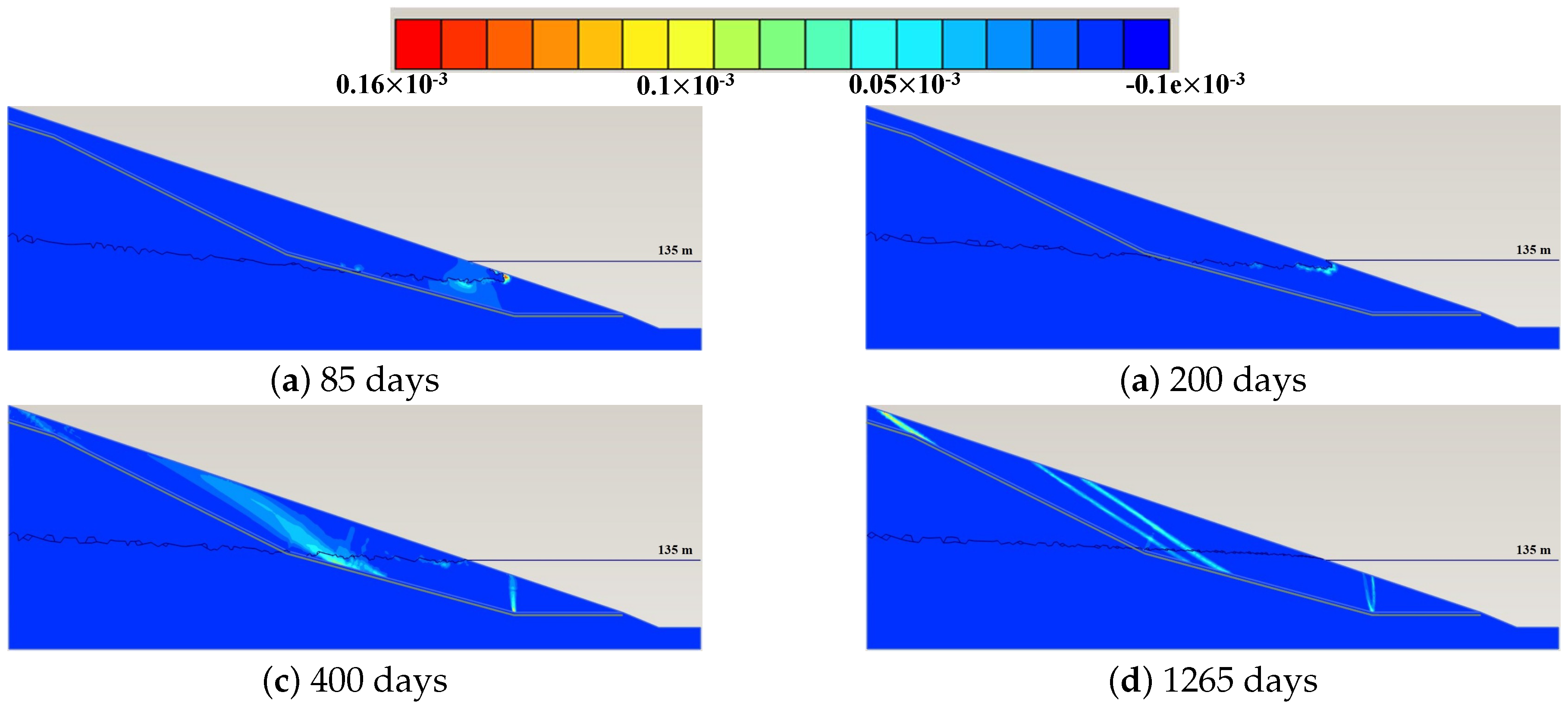
4.1. Pore Water Pressure Evolution
Figure 4 shows the pore water pressure distribution at four different time steps, namely after 85, 200, 400 and 1265 days from the start of the river level rising. It indicates that the pore water pressure cannot reach equilibrium after river level reaches its highest level keeping to be constant in short-term. Due to the large dimension of the slope and the low permeability of the sliding body as well as of the bedrock, the groundwater level in the slope remains unchanged for a short time after the river level fluctuation starts. However, the area near the river is under the influence of rising water levels suddenly, and the groundwater level in this area may rise relatively quickly. Therefore, there is a concave curve of the pore–water pressure isocline nearby the river and slope surface. It is evident that when the water table in the river reaches the level of 135 m, the groundwater level in the slope body cannot stabilize immediately. It takes time for the excess pore water pressure to dissipate and to reach equilibrium. The redistribution of the pore water pressure is dominated by the permeability of the sliding body, and perhaps also depends on the time interval of the river level fluctuation.
In the present case, as shown in Figure 4b,c, the groundwater level still does not reach a stable state compared with the final stable state shown in Figure 4d. In other words, the change of the river level in 85 days can directly influence the pore water pressure distribution for more than 400 days.
4.2. Deformation Evolution
Figure 5 shows the horizontal displacement evolution after 85, 200, 400 and 1265 days after the start of the river level rising. As shown in Figure 5a, when the river level rises and reaches the maximum of 135 m, there is nearly no deformation in the slope body. The deformation is also very small after 200 days when the displacement in the lower part of the sliding body is less than 10 mm. After 400 days, the deformation in sliding body starts to be more evident. The lower part displacements are significantly larger than the displacements in the upper part of the model. The horizontal displacement of the lower part of the sliding body after 400 days is between 30 and 50 mm. After a long-term influence of the higher river level, e.g., after 1265 days, the deformation of the lower part of the sliding body exceeds 130 mm. The evolution and the distribution of the landslide deformation indicate that the deformation of the lower part of the landslide plays a key role in the whole system. In Figure 5d, it can be seen that in the upper part of the sliding body, deformations mainly occur close to the slope surface, and the deformation decreases with depth.
To better explain the shear behaviour of the slope, Figure 6 shows the incremental deviatoric strain evolution in these 1265 days. When the river level quickly rises and reaches its maximum in 85 days, there is nearly no plastic zone in the sliding body (see Figure 6a). This situation remains till 200 days (see Figure 6b). After 400 days (see Figure 6c), two shear bands develop where higher deviatoric strain occurs. One shear zone occurs nearby the toe of the slope, the other locates in the middle of the slope. Both of them are directed from the slope surface to the weak layer 2 indicating that the failure may firstly occur in the lower part of the slope, where the hydraulic regime evolves earlier, and the properties of weak layer 2 may be among the crucial landslide influencing factors. In 1265 days, there is a new shear band with higher deviatoric strain formed in the back of the slope. It indicates that the movement of the upper part of the slope follows its lower part.
According to the above discussion, after the river level starts rising, on the one hand, the slope moves towards the river due to the shear deformation. On the other hand, the water pressure resists the movement of the slope and pushes the slope body away from the river. In short-term (first 85 days), the water cannot fully enter the slope body immediately. Therefore, excess pore water pressure is generated in the slope body. Because the excess pore water pressure cannot dissipate in short-term, the deformation of the slope mainly results from the seepage force, which pushes the material of the slope far away from the river. Therefore, the horizontal displacements at the observation points have negative values.
In the mid-term (85–400 days), the water still evidently enters the slope from the river and the excess pore water pressure starts dissipating. Therefore, the deformation of the slope results from two factors: increasing seepage force and dissipating excess pore water pressure. Because the water keeps entering the slope body in this period, the seepage force also increases, which pushes the material of the slope away from the river. Meanwhile, because the excess pore water pressure dissipates, the material of the slope moves to the river. With the speed of water penetration decreasing, the influence from seepage force is also reducing. Therefore, the influence proportion from dissipating excess pore water pressure gradually increases, which results in a slope movement towards the river.
While in long-term (400–1265 days), the water level in the slope body almost reaches equilibrium. The residual excess pore water pressure gradually dissipates and this results in dominant shear deformations in the system. Furthermore, it is worth mentioning that the properties of the weak layer 2 play an important role in the slope deformations due to its reduced, compared to the adjacent soil shear strength. This observation will be further discussed in Section 5.
4.3. Influence of the Permeability of the Sliding Body
As it has been already mentioned, the permeability of the involved materials can directly control the rate of water flow in the slope where the water level varies. In this study, the sliding body is simplified to be composed of a homogeneous material with an assumed average value of the permeability (see Table 1). However, in reality, the sliding body is composed of many different materials whose permeability values vary within a large range. Therefore, the influence of the uncertainty in the permeability has to be considered. In this section, ten different values of permeability of the sliding body varying from 4.6 × 10 m/s to 4.6 × 10 m/s are employed, meanwhile, other parameters are all kept constant. The comparison of the different model responses depending on the sliding body permeability can indicate the importance of the value of the permeability of the sliding body. Figure 7 shows the variation of the horizontal displacement evolution at G7 (Figure 7a) and G9 (Figure 7b) depending on the sliding body permeability. To observe the correlation between permeability and deformation in short-term, Figure 7c,d show the dependence of the horizontal displacement evolution from permeability in the two observation points G7 and G9 after 85 and 200 days from the start of river level rising.
The general trend of the relation between deformation and permeability is that the deformation decreases with increasing the permeability of the sliding body. This happens because when the permeability of soil is quite large, the water can penetrate into soil and dissipate very quickly, which generates smaller excess pore water pressure. The effective stress in the slope body is relatively larger for higher values of the soil permeability. Therefore, with higher permeability, the model contains fewer plastic points, the deformation is smaller and the slope is more stable.
As shown in Figure 7c,d, when the river level quickly increases during the first 85 days, the displacements at G7 and G9 are almost zero. In the area around the observation point G7, where is very close to the region submerged due to the river level uprises, on one hand, the rising water level can result in larger resistance force due to wider stress distribution on the toe of the slope, which increases the stability of the landslide. On the other hand, the quickly rising water level could increase the weight of the slope, which increases the sliding force and the excess pore water pressure in the slope body, which decreases the effective stress and instabilises the slope. For the lower permeability values, larger excess pore water pressure is generated and the slope tends to instabilise. On the contrary, the slope is more stable and the flow force can push the soil far away from the river. The negative displacements shown in Figure 7c indicate that the material is moving away from the river.
As regarding the results at the observation point G9, because it is relatively far away from the river bank, it appears the model response there to be less influenced by the pore water pressure variation. The movement of G9 is mainly dominated by the movement of the lower region close to the river. The trend of the displacement evolution at G9 follows the one at G7, but the effect of permeability on the deformation is much smaller.
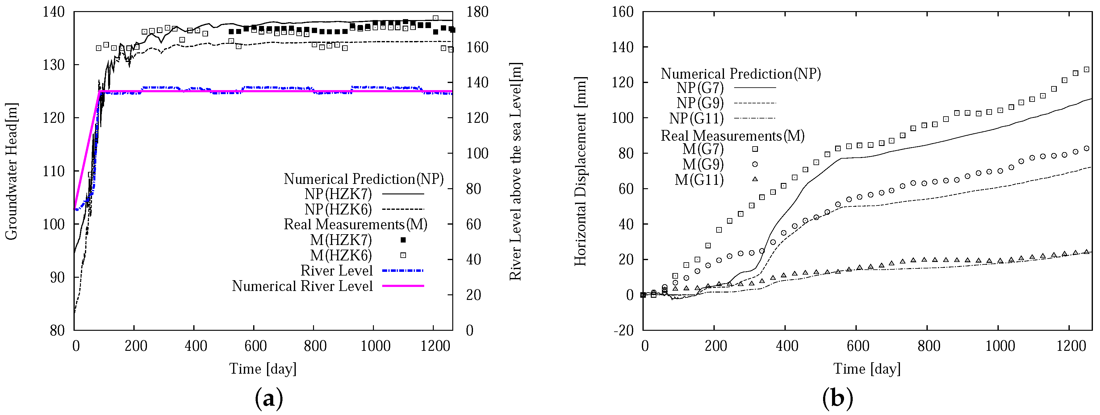
4.4. Comparison between the Numerical Prediction and the Real Measurement
In the numerical simulation in this subsection, the model parameters are selected according to Table 1. Figure 8 shows the comparison for both groundwater level (HZK6 and HZK7) and horizontal displacements (G7, G9, G11) between the numerical results and the real measurement (locations of the observation points are shown in Figure 3). The comparison of the groundwater level reveals that at the observation point HZK7, the numerical results exceed the measurements. At the observation point HZK6, before 400 days, the measurements have higher values than the numerical results. It indicates that the groundwater level in reality rises more quickly than it is predicted by the numerical model. After 400 days, the numerical results eventually keep constant. On the contrary, the groundwater level in reality still fluctuates. The lowest water level is about 133 m and highest water level is around 137 m. The numerical results are closer to the lower boundary for the measured groundwater level at point HZK6, but they slightly overestimate the in situ minimal water level data.
Regarding the comparison of the simulated and measured horizontal displacements in Figure 8b, after 400 days, the evolution of measured deformation and the model prediction are almost identical. There is also a good agreement between the measurements and model outputs at the observation point G11. However, at points G7 and G9, there are still relatively large differences between the measurements and the numerical results, especially at smaller time steps.
The measurements show that the displacement should gradually increase after the water level starts rising. However, the numerical results indicate that there are nearly no displacements at G7, G9, G11 before 200 days. The displacements at observation points start increasing after about 200 days and increase much more rapidly in comparison to the monitored displacements.
There are two possible reasons for the discrepancy between the measurements and the model predictions. On one hand, the used current numerical model is oversimplified, and therefore it cannot fully simulate the reality. For instance, the sliding body in the numerical modelling is assumed to be composed of a homogeneous material, and the material parameters for the sliding body are approximate values considering the corresponding parameters of different materials that make up the real slope. The model outputs may eventually fit the real slope response after a proper modification of the model parameters. In the following, we examine the reason for the model’s mismatch with reality and try to modify the current numerical model in order to get a better match between the model and the reality.
5. Sensitivity Analysis
According to the above discussion, there is large discrepancy between the numerical prediction and the real measurements. On the one hand, the discrepancy might be due to the factors which are not considered in the numerical modelling, such as the inhomogeneity of the slope, rainfall, temperature variation, etc. On the other hand, it might be due to the parameter uncertainties. The parameters of survey report just represent certain local points, and the uncertainties of the parameters must be taken into account. In addition, the inaccuracy of experiments may also cause the parameter uncertainties. In this study, to reduce the uncertainty involved in the soil parameters, a sensitivity analysis can be performed as a powerful tool to distinguish the relative importance of model inputs in determining the model responds (e.g., displacement, pore water pressure and etc.). Sensitivity analysis can evaluate the importance of each uncertain parameter to the model responses. The results of sensitivity analysis cannot only be used to evaluate the relative importance of model parameters, but also be used to decrease the dimension of the back analysis. Saltelli [23] introduced the motivation of sensitivity analysis, presented the fundamental theory of sensitivity analysis and gave several practical illustrations. Sobol [24] employed Monte-Carlo algorithm to estimate the sensitivity of a function with respect to arbitrary variable sets. The sensitivity analysis has been widely applied in many geotechnical engineering problems. Khaledi et al. [25] applies numerical modelling for salt caverns and used global sensitivity analysis to investigate the influence of material parameters on the mechanical behaviour of the salt cavern. Mahmoudi et al. [26] provides a reliability-based analysis of a typical renewable energy storage cavern in rock salt, and sensitivity analysis for different variables involved in the mechanical response of cavern is conducted by global sensitivity method. Miro et al. [27] conducted Variance-based global sensitivity analysis for quantifying the impact of each uncertain parameter on different system responses. Currently, there are two widely used concepts for sensitivity analysis, namely local sensitivity analysis (LSA) and global sensitivity analysis (GSA). Zhao et al. [28] adopts the local and global sensitivity analyses to study the influence of the soil-tunnel-building system characters on the settlement and tilt of building. The results are used to properly update the design parameters during tunnel construction. In this section, both of the two methods will be introduced.
5.1. Local Sensitivity Analysis
Local sensitivity analysis is normally used to investigate the effect of the small variation of model parameters. It is applied in a small space around a given point in parameter space. In this study, the scaled sensitivity indicates the variation of ith observation with the change of the jth parameter . It is calculated as according to:
The overall model sensitivity to the jth parameter is named as composite scaled sensitivity () and it is defined as:
To compare the composite scaled sensitivity of different model parameters, the ratio is defined as follows:
It is evident that the ratio of the most important parameter is equal to 1 and the parameter with larger ratio is relatively more important over the considered model parameter space. Even though the applicability of LSA method is limited, for instance, the LSA results might be questionable when the inputs are non-linearly related to the model outputs or when the range of the model inputs variation is very large, the LSA method is still a powerful and economic tool to obtain a preliminary assessment of the relative importance of the model parameters.
In this study, because the bedrock can be considered as a homogeneous material, and thought to be well investigated, the permeability of the bedrock is set to be a known and constant value. To reduce the dimension of the model parameter set, it is assumed that = , and = 3 for the sliding body. The exponent power and Poisson’s ratio of the sliding body are also set to have known constant value.
Nine parameters are chosen to be considered in the LSA, and they are shear strength of the weak layer 1, the weak layer 2 and the sliding body (, , , , , ), the permeability and the reference secant modulus of the sliding body (k, ), and the hydrostatic water head at the left boundary (H). These model parameters are expected to be most influential to the model response based on an engineering judgment. The reference point in the parameter space is the set given in Table 1. In the present LSA, the step size of varying each variable is chosen to be 10%. It has to be ensured that the truncation and condition errors of the numerical simulation are less influential than the effect of model parameters variation [13].
5.2. Global Sensitivity Analysis
The Global Sensitivity Analysis (GSA) is employed to investigate how the variation in the output of a numerical model can be attributed to variations of its inputs. The reason to perform a GSA in addition to the LSA is, firstly, because the LSA becomes inaccurate when the relation between the model response and inputs is non-linear. The GSA method measures the sensitivity of model response throughout the whole parameter space and it can deal with nonlinear models. Secondly, the correlation among model parameters can be also evaluated by means of the GSA. In this study, the Variance-Based GSA is adopted, according to Saltelli [23]. The sample points are generated with Monte-Carlo sampling method, which are assumed to uniformly distribute in the whole parameter space. The first order index S and the total effect index S are calculated as [23]:
where A and B are two independent matrices, each containing n random samples of the input parameters vector X. The matrix Cj is a matrix whose columns are the same as those of the matrix B except the jth column which is the same as the jth column of the matrix A. The vectors y, y, y are the vectors of the model response corresponding to the parameter sets in A, B and Cj. Finally, and are the mean values of y and y, respectively.
The GSA needs extensive calculations involving thousands of samples, and therefore, a large number of solutions of the forward model. It is unrealistic to solve so many times the forward numerical problem since a simulation takes a relatively long time because we have a large-scale model of extreme design. This difficulty can be overcome by using metamodellilng approach to acquire approximate model output and thus to save calculation time. In general, a metamodel or surrogate model is a mathematical model that evaluates the behaviour of a multivariate complex system while it is computationally inexpensive. All metamodelling techniques consist of running the original but computationally expensive simulation on a set of samples and using the gained information to predict the result of running the simulation at other points in the parameters’ space. The surrogate model needs n vectors of k input parameters sampled randomly in the k-dimensional parameters’ space to generate n vectors of system responses for training the metamodel. Depending on the structure of input parameters set and the system behaviour, several approximation techniques may be applied (Bolzon and Buljak [29], Lancaster and Salkauskas [30], Matheron [31], Powell [32]). In this study, Proper Orthogonal Decomposition (POD) combined with Radial Basis Functions (RBF) is used in the metamodelling strategy to solve the optimisation problem and to run a large number of evaluations of the defined objective function. POD-RBF is proposed in Buljak [33] to build a metamodel for scattered points in a multidimensional space. The method finds the projection of the system response into a reduced space and then an approximation is carried out by using radial basis functions. Examples for the application of metamodelling techniques in geotechnical engineering are shown in e.g., Khaledi et al. [34]. In this study, the range of parameters variation (lower and upper bounds) determined based on in situ reports and engineering judgement are given in Table 2. The parameters in this range must ensure that the model gives reasonable outputs, by which a high quality metamodel can be created. In the considered parameter range, a total of 200 samples are generated to create the metamodel and 50 samples are generated to test the quality of the created metamodel. The approximation accuracy of the metamodel for the horizontal displacements at G7 and G9 is 0.962 and 0.962, respectively.
5.3. Results of the Local Sensitivity Analysis
The results of the LSA for the final horizontal displacement (at points G7 and G9) and groundwater level (at points HZK6 and HZK7) are given in Figure 9. As shown in Figure 9, hydrostatic water head could be most important to both horizontal displacement and groundwater head in the considered parameter space. The hydrostatic water head at the left boundary dominates the initial pore water pressure and the stress distribution of the model, what in turn significantly affects the system behaviour when the river level rises up. Meanwhile, model responses are also highly sensitive to the permeability of the sliding body. The pore water pressure distribution with varying water level is mainly dominated by the permeability of the sliding body, which in term significantly influences the values of the effective stress. In addition, of the weak layer 2 and the shear strength parameters and of the sliding body are more important compared to the other parameters. This is because the plastic deformations in the soil are dominated by these strength parameters. Based on the LSA results, it can be concluded that the model outputs are poorly sensitive to the shear strength of the weak layer 1. Obviously, the deformation of the lower part of the slope body is the key part of the entire deformation of the model. Due to the fact that the weak layer 1 is located further away from the river than the weak layer 2, the shear strength of the weak layer 1 is therefore less important as compared to the shear strength of the weak layer 2. Lastly, the model responses (e.g., displacement and pore water pressure) at the given observation points is not sensitive to . Based on the LSA results, five parameters, , , , k and H, can be considered as candidates for the GSA and for the optimisation procedure as these parameters have a significant influence on the model output.
5.4. Results of the Global Sensitivity Analysis
The lower and upper bounds for GSA of five chosen parameters are given in Table 2. Figure 10 presents the sensitivity of landslide behaviour to the model parameters in the whole parameter space. Figure 10a shows the sensitivity of horizontal displacement at G7 and G9, and Figure 10b shows the sensitivity of groundwater level at HZK 6 and HZK7. Figure 10a indicates that the most important parameter for the horizontal displacements is (the friction angle of the weak layer 2). The friction angle of the lower weak layer significantly dominates the horizontal displacements at both G7 and G9. As mentioned in Section 4.2, there is a main sliding band generated in the middle of the sliding body, and the bottom of the band reaches the weak layer 2. Meanwhile, there is also a small sliding belt generated close to the toe of the slope, which also approaches the weak layer 2. Because the friction angle of the weak layer 2 is much smaller than the one of the sliding body, the stress points at the interface elements more easily reach the plastic zone. The irreversible plastic deformation of the weak layer 2 drives the deformation of the whole system. Therefore, the shear strength of the weak layer 2 significantly dominates the deformation of the sliding body.
Meanwhile, the permeability of the sliding body also plays a key role in the deformation of the slope. As mentioned before, the permeability of the sliding body significantly influences the effective stress, which in turn affects the soil deformation. In addition, the deformation is also sensitive to the parameters and H, but these two parameters are not as dominant as and k. Lastly, is almost not influential to the deformation of the model.
Figure 10b shows that k of the sliding body and H play key role in the numerical modelling for the groundwater level, and the other three parameters, , and , are almost not influencing the groundwater level changes.
As shown in Figure 9 and Figure 10, there is obvious difference in the ranking of the important parameters obtained from LSA and GSA. In LSA, H is the most important parameter for both deformation and groundwater level changing, and also plays a quite important role. However, in GSA, for deformation, H is less important than and k; for groundwater level, H is important, but it is not as important as k. In addition, the model outputs are nearly not sensitive to the parameter .
This difference between the LSA and GSA results can be explained in two aspects. Firstly, in LSA, the parameter set varies only in a very small region around the predefined parameter value, and the scaled sensitivity to a parameter is calculated through a linear approximation. Therefore, the result of the LSA is only reliable in a very small parameter space around given reference parameter set. On the contrary, the GSA considers the parameter variation throughout the whole parameter space. It is also reliable when the correlation between the model outputs and inputs is non-linear. Moreover, the GSA can also evaluate the coupling effects among parameters, in other word, it can indicate the uncertainty contribution from the correlated variations of other parameters. Therefore, the GSA is thought to be more reliable to evaluate the importance of model inputs accounting the whole parameter space.
6. Parameter Identification Through Back Analysis
As mentioned in Section 4, there is a huge difference between numerical prediction and real measurement. In Section 5, the model responses are thought to be sensitive to five parameters (, , , k and H). To obtain the optimal parameter set which can give a good prediction compared with real measurements, the back analysis is adopted. To evaluate the prediction ability of the calibrated model, model verification is also performed in this section.
6.1. Methodology
Back analysis is applied for model calibration and it aims to minimize the difference between the computed results via finite element simulation and the real measurements. In our case, the identified parameters should minimize the following objective function:
where and are the model prediction and the measured values; m represents the number of measurement points, n is the number of time steps. In this paper, the genetic algorithm (GA) is chosen for minimizing the objective function. The GA is well accepted as a powerful and economical algorithm to minimize the objective function. It has received substantial attention in engineering design optimisation in the recent decades [35]. The Genetic algorithm is a population-based algorithm, inspired by Darwin’s evolution theory [36]. It simulates a population of creatures randomly; each of individuals among this population represents a point in a search space and a possible solution to solve optimisation problems. Then, it finds the fittest among individuals over consecutive generation, what corresponds to that model responses that fits best to the measurements, and uses them to create the individuals for the next generation. For the purpose of the back analysis, the built metamodel for the GSA is used to substitute the Finite element model in order to reduce the computational time cost.
For the analysis hereafter, we choose two observation points (G7 and G9) and in this case m = 2; while n = 1, as we only look at the results in one fixed time step, namely the middle of the entire time interval (610th days). The obtained optimal parameter set is tabulated in Table 3. However, because the objective function is defined only with , at the time step of the 610th day, the determined ’optimal’ parameters might not assure satisfactory fit of the measured data in larger time span. Therefore, the quality of the calibrated model is subject to verification. The verification procedure use the results of the finite element simulation with the ’optimal’ parameters, listed in Table 3 as input model parameters. The evaluation criterion is again the mean relative error between model prediction and real measurements at 10 specific time steps between 500 days and 800 days (519, 549, 580, 610, 641, 672, 700, 731, 761, 792 days). The new judgment equation is same as formulas in Equation (6), and it is still calculated in accordance with the same observation points G7 and G9. Where, n = 10 and m = 2.
To evaluate the prediction ability of the employed model, in this paper, the evaluation criterion is defined as the relative error between model prediction and real measurements at 6 specific time steps between 800 days and 1265 days for horizontal displacement at G7, G9, G11. The horizontal displacement at G11 is also employed to evaluate the prediction ability. The evaluation function is same as formulas in Equation (6), and where n = 6 and m = 3. The specific time step is assumed at 822, 914, 1006, 1096, 1187, 1249 days.
6.2. Results of Parameter Identification and Model Verification
Table 3 shows the optimal parameter set. As shown in Table 3, between 500 and 800 days, the mean relative error of initial model is 0.157. Due to the back analysis, the goodness of fit is improved and the mean relative error of the model response against the measured data drops to 0.085. In the next step, the horizontal displacement at observation point G11 is also involved. The results show that the prediction ability after 800 days of the calibrated model is still quite good. The mean relative error is 0.0536, while the corresponding mean relative error using the initial guess for the model parameters is higher.
Figure 11 shows the comparison between finite element model results and measurement data before and after back analysis. Figure 11a presents the comparison between the results for the groundwater level at HZK6 and HZK7 employing the optimal and the initial parameter values. It is evident that after about 500 days the numerical results remain almost unaffected by the change of the input parameters indicating that the pore water pressure distribution reaches a stationary state. However, after 500 days the real measurements show slight fluctuations, especially at point HZK6, where the difference between the largest and smallest measured values after the 500th day is about 4 m. This fluctuation is probably due to seasonal climate changing that is not captured by the current numerical model. Regarding the groundwater level evolution, the numerical results for the groundwater level after the back analysis are lower than these before the back analysis. After 500 days, the numerical results at point HZK7 show a fairly good agreement with the measurements. However, for the observations in point HZK6, there is an agreement only between the results after the back analysis and the measurements at lower values in the measurement band. The reason is probably again in that the factor of seasonal climate changing is not considered in the presented numerical simulation. Before 500 days, only the groundwater level at HZK6 is measured, and the measurement data is evidently higher than model predictions. As it has been already mentioned, the pore water pressure up to the 500th day is not stable and it is significantly dominated by the permeability. In our analysis, the sliding body is considered to consist of a homogeneous material, which is not realistic. Since the measurements over the first 500 days exceed the numerically predicted values near the river where HZK6 is located, it can be assumed that the permeability in the area around the river bank might be slightly increased. Therefore, the model needs to be further improved considering more in detail the materials of the sliding body and eventually suggesting the use of different permeabilities for the involved materials.
Figure 11b shows the comparison of the horizontal displacements at G7, G9 and G11. It is evident that for long-term prediction, the model response employing the optimal parameter set is significantly improved compared to the performance of the initial model. There is a good agreement especially after 800 days at all observation points. In the time period from 500 days to 800 days, the goodness of fit of the improved model is still acceptable. However, during the first 500 days, there is only good agreement between the model and the measurements for point G11. The predicted horizontal displacements at G7 and G9 are always below the measurements. Concluding, the analysis indicates that the model can simulate and predict the processes in the regions away from the river very good. However, close to the river, the numerical model still needs to be improved.
As discussed in Section 5, the shear strength parameters of the materials of the sliding body and the weak layer 2, as well as the permeability of the sliding body are all significantly influencing the model deformation. As mentioned in Section 4, lower permeability of the sliding body could increase the deformation of the slope body. By contrast, to get a better fit of the groundwater level data, the permeability should be increased. This contradiction may indicate that to fit the displacement evolution, permeability is not the key factor. Based on the discussion and the description in Section 2, there is existing smaller weak zone in the sliding body, which are not considered in current numerical model. That means in the next stage, weaker layers in the sliding body close to the river should be added to the model. In addition, some other factors, such as precipitation, temperature variation and etc., might be included to improve the model prediction quality.
Lastly, because the current model has acceptable fitting quality and prediction ability for the regions far away from the river, the corresponding part of the numerical model can be kept as it is when further improving the mathematical model. Because the current model can well predict the landslide behaviour in long-term with constant water level, the current constitutive model, namely the HS model, is approved to be a reliable material model.
7. Conclusions and Discussion
The paper numerically studies the behaviour of Huangtupo landslide under the influence of fluctuating water level. Both deformation and groundwater level variation have been investigated. To analyse which soil parameters have more dominant influence on the model responses and to reduce parameter dimension of further model calibration, sensitivity analysis is employed. By performing back analysis, the optimised parameter set is found, and adopted to the model to evaluate the goodness of fit between the numerical results and measurements from 500 to 800 days for deformation of the landslide, and it is also used to verify the prediction ability of the calibrated model after 800 days. The following conclusions can be made based on the main findings of present study:
- The pore water pressure in the slope cannot reach equilibrium in short-term when the water level quickly rises and reaches highest level. This procedure is mainly dominated by the permeability of the sliding body.
- The deformation of lower part of the landslide is much larger than that of the upper part. It was found that the deformation of lower part drives the deformation of the whole system. When the river level quickly rises, there is nearly no deformation in the sliding body. It means that in short-term after river level starts rising, the higher river level can resist the movement towards the river. In long-term, the deformation is mainly because of consolidation.
- Results of local sensitivity analysis (LSA) revealed that assumed hydrostatic water head at the uphill boundary and the cohesion of the sliding body are very important to the model responses. The model responses are also sensitive to permeability and friction angle of the sliding body and the friction angle of the weak layer 2. On the contrary, the results of global sensitivity analysis (GSA) indicate that the model deformation is most sensitive to the friction angle of the weak layer 2, and groundwater level variation is most sensitive to the permeability of the sliding body. LSA is valuable to filter out unimportant factors in the preliminary stage and to reduce the dimension of back analysis problem.
- The quality of fit in mid-term of this simulation (500–800 days) is good, and the prediction ability after 800 days of the model is also satisfactory. It shows that the simplified model can well simulate long-term behaviour of the landslide after the river level reaches the top level.
- There is still space to improve the numerical prediction of the short-term slope deformation. The discrepancy of groundwater levels between numerical prediction and real measurements is because of the assumed average permeability of the model’s lower part. The discrepancy of landslide deformation between numerical prediction and real measurements is because that the sliding body is considered as homogeneous material in this study, and some weaker zones in the lower part of the sliding body are not considered.
- In further research, the part far away from the river of the numerical model can be kept, the lower part of the sliding body can be divided into more layers based on real material distribution. In addition, some other factors, such as rainfall, temperature variation, etc. might also be employed to improve the model.
Author Contributions
X.L., C.Z. performed the numerical simulations; R.H., X.L., and C.Z. did the sensitivity analysis; X.L., C.Z., R.H., A.A.L. and M.D. analysed the results; X.L. drafted the manuscript, and C.Z., R.H., A.A.L. and M.D. edited the manuscript.
Funding
This research is supported by Three Gorges Research Center for Geoharzards (Ministry of Education, China) and German Research Foundation (DFG) through collaborative research center SFB 837 (subprojects A5 and C2). The first author is sponsored through a scholarship by the China Scholarship Council (CSC).
Acknowledgments
The authors express their sincerest reverence to Professor Tom Schanz who passed away during this study, for his valuable scientific contribution, careful guidance, helpful suggestions and constructive discussions. We also acknowledge support by the DFG Open Access Publication Funds of the Ruhr-Universität Bochum.
Conflicts of Interest
The authors declare no conflict of interest.
References
- Cai, Y.; Guo, Q.; Yu, Y. The reservoir-induced slope failure mechanism and prediction. Hubei Geol. Miner. Resour. 2002, 16, 4–7. [Google Scholar]
- Wang, F.; Zhang, Y.; Huo, Z. Mechanism for the rapid motion of the Qianjiangping landslide during reactivation by the first impoundment of the Three Gorges Dam reservoir. Landslide 2008, 5, 379–386. [Google Scholar] [CrossRef]
- He, K.Q.; Li, X.R.; Yan, X.Q. The landslides in the Three Gorges Reservoir Region, China and the effects of water storage and rain on their stability. Environ. Geol. 2008, 55, 55–63. [Google Scholar]
- Wu, S.R.; Jin, Y.M.; Zhang, Y.S. Investigations and assessment of the landslide hazards of Fengdu County in the reservoir region of the Three Gorges project on the Yangtze River. Environ. Geol. 2004, 45, 560–566. [Google Scholar] [CrossRef]
- Kilburn, C.R.J.; Petley, D.N. Forecasting giant, catastrophic slope collapse: Lessons from Vajont, Northern Italy. Geomorphology 2003, 54, 21–32. [Google Scholar] [CrossRef]
- Borgatti, L.; Corsini, A.; Barbieri, M.; Sartini, G.; Truffelli, G.; Caputo, G.; Puglisi, C. Large reactivated landslides in weak rock masses: A case study from the Northern Apennines (Italy). Landslide 2006, 3, 115–124. [Google Scholar] [CrossRef]
- Ronchetti, F.; Borgatti, L.; Cervi1, F.; Gorgoni, C.; Piccinini, L.; Vincenzi, V.; Corsini, A. Groundwater processes in a complex landslide, northern Apennines, Italy. Nat. Hazards Earth Syst. Sci. 2009, 9, 895–904. [Google Scholar] [CrossRef] [Green Version]
- Chien, L.; Hsu, C.; Yin, L. Warning Model for Shallow Landslides Induced by Extreme Rainfall. Water 2015, 7, 4362–4384. [Google Scholar] [CrossRef] [Green Version]
- Matsuura, S.; Asano, S.; Okamoto, T. Relationship between rain and/or meltwater, pore-water pressure and displacement of a reactivated landslide. Eng. Geol. 2008, 101, 49–59. [Google Scholar] [CrossRef]
- Qi, S.; Yan, F.; Wang, S.; Xu, R. Characteristics, mechanism and development tendency of deformation of Maoping landslide after commission of Geheyan reservoir on the Qingjiang River, Hubei Province, China. Eng. Geol. 2006, 86, 37–51. [Google Scholar] [CrossRef]
- Jia, G.W.; Zhan, T.L.T.; Chen, Y.M.; Fredlund, D.G. Performance of a large-scale slope model subjected to rising and lowering water levels. Eng. Geol. 2009, 1–2, 92–103. [Google Scholar] [CrossRef]
- Yan, Z.; Wang, J.; Chai, H. Influence of water level fluctuation on phreatic line in silty soil model slope. Eng. Geol. 2010, 113, 90–98. [Google Scholar] [CrossRef]
- Zhao, J.; Yu, J.; Xie, M.; Chai, H.; Li, T.; Bu, F.; Lin, B. Physical model studies on fill embankment slope deformation mechanism under rainfall condition. Rock Soil Mech. 2018, 39, 2933–2940. [Google Scholar]
- Chen, S.; Xu, G.; Chen, G.; Wu, X. Research on engineering geology characteristics of soil in sliding zone of Huangtupo landslide in Three Gorges Reservoir area. Rock Soil Mech. 2009, 30, 3048–3052. [Google Scholar]
- Wang, J.; Xiang, W.; Lu, N. Landsliding triggered by reservoir operation: A general conceptual model with a case study at Three Gorges Reservoir. Acta Geotech. 2014, 9, 771–788. [Google Scholar] [CrossRef]
- Jian, W.; Xu, Q.; Yang, H.; Wang, F. Mechanism and failure process of Qianjiangping landslide in the Three Gorges reservoir, China. Environ. Earth Sci. 2014, 72, 2999–3013. [Google Scholar] [CrossRef]
- Jiang, J.W.; Ehret, D.; Xiang, W. Numerical simulation of Qiaotou Landslide deformation caused by drawdown of the Three Gorges Reservoir, China. Eng. Geol. 2011, 62, 411–419. [Google Scholar] [CrossRef]
- Hu, X.; Tang, H.; Li, C.; Sun, R. Stability of Huangtupo riverside slumping mass under water level fluctuation of Three Gorges Reservoir. Eng. Geol. 2012, 23, 326–334. [Google Scholar] [CrossRef]
- Marcato, G.; Mantovani, M.; Pasuto, A.; Zabuski, L.; Borgatti, L. Monitoring, numerical modelling and hazard mitigation of the Moscardo landslide (Eastern Italian Alps). Eng. Geol. 2018, 128, 95–107. [Google Scholar] [CrossRef]
- Lei, D.; Yi, W.; Liu, Q.; Xia, J. Reliability and sensitivity analysis of Woshaxi landslide stability in three gorges reservior area. Saf. Environ. Eng. 2002, 25, 23–28. [Google Scholar]
- Hubei Survey and Design Institute for Geo-Hazard. Survey Report of Huangtupo Landslide in Three Gorges Reservoir Area, BaDong, Hubei Province, China; Technical Report; Hubei Survey and Design Institute for Geo-Hazard: Wuhan, China, 2001. (In Chinese) [Google Scholar]
- Schanz, T.; Vermeer, P.; Bonnier, P. The hardening soil model: Formulation and verification. In Proceedings of the 1st International PLAXIS Symposium on Beyond 2000 in Computational Geotechnics, Amsterdam, The Netherlands, 18–20 March 1999; pp. 281–296. [Google Scholar]
- Saltelli, A. Global Sensitivity Analysis; John Wiley and Sons: Hoboken, NJ, USA, 2008. [Google Scholar]
- Sobol’, I.M. Sensitivity estimates for nonlinear mathematical models. Math. Model. Comput. Exp. 1993, 1, 407–414. [Google Scholar]
- Khaledi, K.; Mahmoudi, E.; Datcheva, M.; Koenig, D.; Schanz, T. Sensitivity analysis and parameter identification of a time dependent constitutive model for rock salt. J. Comput. Appl. Math. 2016, 293, 128–138. [Google Scholar] [CrossRef]
- Mahmoudi, E.; Khaledi, K.; Miro, S.; Koenig, D.; Schanz, T. Probabilistic Analysis of a Rock Salt Cavern with Application to Energy Storage Systems. Rock Mech. Rock Eng. 2017, 50, 139–157. [Google Scholar] [CrossRef]
- Miro, S.; Koenig, M.; Hartmann, D.; Schanz, T. A probabilistic analysis of subsoil parameters uncertainty impacts on tunnel-induced ground movements with a back-analysis study. Comput. Geotech. 2015, 68, 38–53. [Google Scholar] [CrossRef]
- Zhao, C.; Lavasan, A.A.; Hoelter, R.; Schanz, T. Mechanized tunneling induced building settlements and design of optimal monitoring strategies based on sensitivity field. Comput. Geotech. 2018, 97, 246–260. [Google Scholar] [CrossRef]
- Bolzon, G.; Buljak, V. An effective computational tool for parametric studies and identification problems in materials mechanics. Comput. Mech. 2011, 48, 657–687. [Google Scholar] [CrossRef]
- Lancaster, P.; Salkauskas, K. Surfaces generated by moving least squares methods. Math. Comput. 1981, 37, 141–158. [Google Scholar] [CrossRef]
- Matheron, G. Principles of geostatistics. Econ. Geol. 1963, 58, 1246–1266. [Google Scholar] [CrossRef]
- Powell, M. Radial Basis Functions for Multivariable Interpolation: A Review. In Algorithms for Approximation; Oxford University Press: New York, NY, USA, 1987; Chapter 3; pp. 141–167. [Google Scholar]
- Buljak, V. Proper orthogonal decomposition and radial basis functions algorithm for diagnostic procedure based on inverse analysis. FME Trans. 2010, 38, 129–136. [Google Scholar]
- Khaledi, K.; Schanz, T.; Miro, S. Application of metamodelling techniques for mechanize tunnel simulation. J. Theor. Appl. Mech. 2014, 44, 45–54. [Google Scholar] [CrossRef]
- Andrab, S.G.; Hekmat, A.; Yusop, Z.B. A Review: Evolutionary Computations (GA and PSO) in Geotechnical Engineering. Comput. Water Energy Environ. Eng. 2017, 6, 154–174. [Google Scholar] [CrossRef]
- Holland, J.H. Adaptivity in in Natural and Artificial Systems; University of Michigan Press: Ann Arbor, MI, USA, 1975. [Google Scholar]
Figure 1.
(a) Location of the Three Gorges project and the Huangtupo landslide; (b) Map showing the four distinct landslides; (c) Cross section along A–A’ through the No. 1 slide (Wang et al. [15]).
Figure 1.
(a) Location of the Three Gorges project and the Huangtupo landslide; (b) Map showing the four distinct landslides; (c) Cross section along A–A’ through the No. 1 slide (Wang et al. [15]).

Figure 2.
(a) Measured horizontal displacements after the impoundment of the Three Gorges project. (b) Groundwater level monitoring and river level variation.
Figure 2.
(a) Measured horizontal displacements after the impoundment of the Three Gorges project. (b) Groundwater level monitoring and river level variation.

Figure 3.
Numerical model geometry and finite element discretisation.

Figure 4.
Pore water pressure evolution at different time steps after the river level starts rising.
Figure 4.
Pore water pressure evolution at different time steps after the river level starts rising.

Figure 5.
Evolution of the horizontal displacement at different time steps after the river level starts rising.
Figure 5.
Evolution of the horizontal displacement at different time steps after the river level starts rising.

Figure 6.
Evolution of the incremental deviatoric strain at different time steps after the river level starts rising.
Figure 6.
Evolution of the incremental deviatoric strain at different time steps after the river level starts rising.

Figure 7.
Influence of permeability of the sliding body to (a) horizontal displacement at G7, (b) horizontal displacement at G9, (c) horizontal displacement at G7 (after 85 and 200 days), (d) horizontal displacement at G9 (after 85 and 200 days).
Figure 7.
Influence of permeability of the sliding body to (a) horizontal displacement at G7, (b) horizontal displacement at G9, (c) horizontal displacement at G7 (after 85 and 200 days), (d) horizontal displacement at G9 (after 85 and 200 days).

Figure 8.
Comparison between the numerical prediction (NP) and the real measurement (M) for (a) groundwater level at HZK6, HZK7; (b) horizontal displacements at G7, G9, G11.
Figure 8.
Comparison between the numerical prediction (NP) and the real measurement (M) for (a) groundwater level at HZK6, HZK7; (b) horizontal displacements at G7, G9, G11.

Figure 9.
LSA results for: (a) horizontal displacements at G7 and G9, (b) groundwater level at HZK6 and HZK7.
Figure 9.
LSA results for: (a) horizontal displacements at G7 and G9, (b) groundwater level at HZK6 and HZK7.

Figure 10.
GSA results for: (a) horizontal displacements at G7 and G9, (b) groundwater level at HZK6 and HZK7.
Figure 10.
GSA results for: (a) horizontal displacements at G7 and G9, (b) groundwater level at HZK6 and HZK7.

Figure 11.
Comparison between the numerical prediction and measurement data after the back analysis for: (a) groundwater level at HZK6 and HZK7; (b) horizontal displacement at G7, G9 and G11. (NP—final numerical prediction after back analysis; NP0—initial numerical prediction; M—real measurement).
Figure 11.
Comparison between the numerical prediction and measurement data after the back analysis for: (a) groundwater level at HZK6 and HZK7; (b) horizontal displacement at G7, G9 and G11. (NP—final numerical prediction after back analysis; NP0—initial numerical prediction; M—real measurement).


Table 1.
Initial input parameters of the used constitutive model for different materials.
| Material | Parameter | Description | Value | Unit |
|---|---|---|---|---|
| Unit weight | 27.6 | kN/m | ||
| Bedrock (LE) | E | Young’s Modulus | 4200 | MPa |
| Poisson’s ratio | 0.3 | - | ||
| k | Permeability | 1.2 × 10 | m/s | |
| c | Cohesion | 0.1 | kPa | |
| Weak Layer 1 (MC) | Friction angle | 27 | ||
| c | Cohesion | 3 | kPa | |
| Weak Layer 2 (MC) | Friction angle | 27 | ||
| Unsaturated unit weight | 21.6 | kN/m | ||
| Saturated unit weight | 22.6 | kN/m | ||
| Secant stiffness in triaxial test | 180 | MPa | ||
| Tangent stiffness in oedometer test | 180 | MPa | ||
| Elastic unloading-reloading stiffness | 540 | MPa | ||
| Exponent power | 0.5 | - | ||
| Sliding body (HS) | c’ | Cohesion | 3 | kPa |
| Friction angle | 27 | |||
| Dilatancy angle | 0 | |||
| Poisson’s ratio | 0.2 | - | ||
| Reference stress | 100 | kPa | ||
| k | Permeability | 4.6 × 10 | m/s |
Table 2.
Lower and upper bounds for the input parameters.
| Parameter | Lower Bound | Upper Bound | Unit |
|---|---|---|---|
| 2.4 | 3.6 | kPa | |
| 17.4 | 18.1 | ||
| 26 | 28 | ||
| k | 2.78 | 6.94 | m/s |
| H | 155 | 159 | m |
Table 3.
Model calibration and verification.
| (kPa) | () | () | k (m/s) | H (m) | Error1 (500–800 days) | Error2 (800–1200 days) | |
|---|---|---|---|---|---|---|---|
| Initial Parameter | 3 | 17.7 | 27 | 4.6 | 158 | 0.157 | 0.1166 |
| Optimised parameter | 3.19 | 17.73 | 26.53 | 4.09 | 156.44 | 0.085 | 0.0536 |
© 2019 by the authors. Licensee MDPI, Basel, Switzerland. This article is an open access article distributed under the terms and conditions of the Creative Commons Attribution (CC BY) license (http://creativecommons.org/licenses/by/4.0/).
Share and Cite
MDPI and ACS Style
Li, X.; Zhao, C.; Hölter, R.; Datcheva, M.; Alimardani Lavasan, A. Modelling of a Large Landslide Problem under Water Level Fluctuation—Model Calibration and Verification. Geosciences 2019, 9, 89. https://doi.org/10.3390/geosciences9020089
AMA Style
Li X, Zhao C, Hölter R, Datcheva M, Alimardani Lavasan A. Modelling of a Large Landslide Problem under Water Level Fluctuation—Model Calibration and Verification. Geosciences. 2019; 9(2):89. https://doi.org/10.3390/geosciences9020089
Chicago/Turabian StyleLi, Xiang, Chenyang Zhao, Raoul Hölter, Maria Datcheva, and Arash Alimardani Lavasan. 2019. "Modelling of a Large Landslide Problem under Water Level Fluctuation—Model Calibration and Verification" Geosciences 9, no. 2: 89. https://doi.org/10.3390/geosciences9020089
Note that from the first issue of 2016, this journal uses article numbers instead of page numbers. See further details here.