Impact of a Random Sequence of Debris Flows on Torrential Fan Formation


Faculty of Civil and Geodetic Engineering, University of Ljubljana, 1000 Ljubljana, Slovenia
*
Author to whom correspondence should be addressed.
Geosciences 2019, 9(2), 64; https://doi.org/10.3390/geosciences9020064
Submission received: 20 November 2018
/
Revised: 17 January 2019
/
Accepted: 21 January 2019
/
Published: 29 January 2019
(This article belongs to the Special Issue Mountain Landslides: Monitoring, Modeling, and Mitigation)
Abstract
:Debris flows with different magnitudes can have a large impact on debris fan characteristics such as height or slope. Moreover, knowledge about the impact of random sequences of debris flows of different magnitudes on debris fan properties is sparse in the literature and can be improved using numerical simulations of debris fan formation. Therefore, in this paper we present the results of numerical simulations wherein we investigated the impact of a random sequence of debris flows on torrential fan formation, where the total volume of transported debris was kept constant, but different rheological properties were used. Overall, 62 debris flow events with different magnitudes from 100 m3 to 20,000 m3 were selected, and the total volume was approximately 225,000 m3. The sequence of these debris flows was randomly generated, and selected debris fan characteristics after the 62 events were compared. For modeling purposes, we applied the Rapid Mass Movement Simulations (RAMMS) software and its debris flow module (RAMMS-DF). The modeling was carried out using (a) real fan topography from an alpine environment (i.e., an actual debris fan in north-west (NW) Slovenia formed by the Suhelj torrent) and (b) an artificial surface with a constant slope. Several RAMMS model parameters were tested. The simulation results confirm that the random sequence of debris flow events has only some minor effects on the fan formation (e.g., slope, maximum height), even when changing debris flow rheological properties in a wide range. After the 62 events, independent of the selected sequence of debris flows, the final fan characteristics were not significantly different from each other. Mann–Whitney (MW) tests and t-tests were used for this purpose, and the selected significance level was 0.05. Moreover, this conclusion applies for artificial and real terrain and for a wide range of tested RAMMS model rheological parameters. Further testing of the RAMMS-DF model in real situations is proposed in order to better understand its applicability and limitations under real conditions for debris flow hazard assessment or the planning of mitigation measures.
1. Introduction
Debris flows are recognized as a type of slope movements of unconsolidated debris taking the form of fairly obvious flows, either fast or slow, wet or dry [1,2]. This “Varnes classification” of landslides received an update in 2014, where debris flow is defined as “very rapid to extremely rapid surging flow of saturated debris in a steep channel and strong entrainment of material and water from the flow path” (landslide type #22 in [3]). These characteristics of debris flows lead to the fact that debris flows cause large economic damage and endanger human lives along their pathways and in their depositional zone (i.e., torrential fans). These relatively flat areas in mountainous regions are usually very attractive habitable or developable land in general, e.g., for settlements and/or agriculture. Hazard assessment of torrential fans is important to avoid high risk and loss or damage and, therefore, to plan adequate prevention measures in the upstream areas (source areas) and/or on torrential fans. For that, good understanding of the governing processes of torrential fans is necessary.
Fans are classified as alluvial fans if they are formed by fluvial processes and as colluvial fans if they are formed by landslide processes including debris flows [4]. As the majority of such fans at the mouth of torrents are formed by a number of processes that vary in time and space, such as debris flows or hyperconcentrated flows, they are most frequently classified as torrential (creek) fans. It is not very easy to recognize fan-forming processes without long historical records or without applying modern dating technologies [5,6].
Many debris fans accumulate material from debris flows, together with debris floods and ordinary fluvial bedload. Evidence used to distinguish debris flow material from other sediment on a fan includes the high slope angle of the fan and very large individual particles, signs of impact loading on obstacles, U-shaped eroded channels, and, of course, steep, debris-loaded channels upstream [3].
It is known that for debris flows that form debris fans, their critical deposition slope and their runout distance in the deposition zone vary with their magnitude and other characteristics [7,8]; this has led to an approach used for hazard assessment of debris fans. Many different methods can be used for the prediction of debris-flow runout on fans, including dynamic simulations using physically based models numerically solving equations of fluid dynamics.
Since a historical combination of debris flows, hyperconcentrated flows, and torrential fluvial bedload events forms not only the surface of present torrential fans, but also their entire sediment (debris) body, it is important to select such a simulation model for debris flow that covers the rheology of fluvial bedload transport as well as debris flow rheology of different debris–water ratios. This study uses the RAMMS simulation model [9] with the debris flow module (called RAMMS:DEBRIS FLOW or RAMMS-DF). This module was developed to simulate the runout of muddy and debris-laden flows in complex terrain. Since its release in 2011, it has been applied for different terrains in Switzerland (Illgraben and Spreitgraben [10]; Richleren, Minstigerbach, Glyssibach and Varuna [11]; Meretschibach and Bondasca [12]), Austria [13], Italy (Southern Apennines [14]), France (Barcelonnette [15,16]), and Norway [17], among others.
In this paper, we report on the application of the RAMMS simulation model for debris fan formation. If we want to generate a debris fan, we need a scenario of its generation, i.e., a sequence of debris flows of different magnitudes and rheological properties. The main scientific question that was investigated in this study was the following: does a random sequence of debris flow events with different magnitudes have a significant impact on the debris fan formation (e.g., average height, elevation distribution)? We defined the order of debris flow events with different magnitudes as a random sequence. In order to provide an answer to this scientific question, we used the simulation model RAMMS with the debris flow module (RAMMS-DF) and applied it to (a) a real torrential fan in alpine environment, i.e., in north-west (NW) Slovenia (i.e., Suhelj fan), and (b) on an artificial terrain with a constant slope. Several RAMMS parameters were tested. The Voellmy parameter sets were defined based on a literature review, using typical values for different environments, not only for alpine environments, in order to test the hypothesis in different environments. Furthermore, t-tests and Mann–Whitney (MW) tests were used to test whether the random sequence of debris flow events has a significant impact on fan formation.
2. Data and Methods
2.1. RAMMS Software
For the purpose of this study, Rapid Mass Movement Simulation (RAMMS) software and its debris flow module were used. RAMMS is a numerical model that can be used for debris flow simulations for practical and research-oriented applications [18]. The model was developed by the WSL Institute for Snow and Avalanche Research SLF. The model uses depth-averaged shallow water equations for granular flows. The frictional characteristics of debris flows are described with a two-parameter Voellmy-fluid friction model since it has been found that it is suitable for the modelling of debris flows. This method separates friction (resistance) into two different parts, namely, viscous–turbulent friction (ξ parameter) and dry–Coulomb friction (µ parameter). Thus, the frictional resistance depends on the velocity vector in the x and y directions, density, slope angle, flow height, and gravitational acceleration [18]. During the simulations, both mentioned parameters are kept constant, but the user can define spatially variable parameters using different polygons. Moreover, newer RAMMS-DF versions that were also used in this study use a modification of the Voellmy equation with the purpose to also include cohesion (yield stress) in the simulations [18]. Furthermore, the model also accounts for the curvature effect (i.e., centrifugal force) [18]. The RAMMS user manual suggests performing model calibration in order to derive suitable Voellmy parameters. In some cases, calibration should be performed separately for different events because RAMMS-DF uses a single-phase model [18]. The RAMMS-DF model includes two options for the input debris flow definition that were also used in this study, namely, a block release option and an input hydrograph option. A detailed RAMMS model and debris flow module description can be found in references [9,13,16,18,19,20,21,22,23]. In this study we investigated two case studies, namely, a real torrential fan named the Suhelj fan (described in Section 2.2) and artificial terrain with a constant slope (described in Section 2.3).
2.2. The Suhelj Torrential Fan
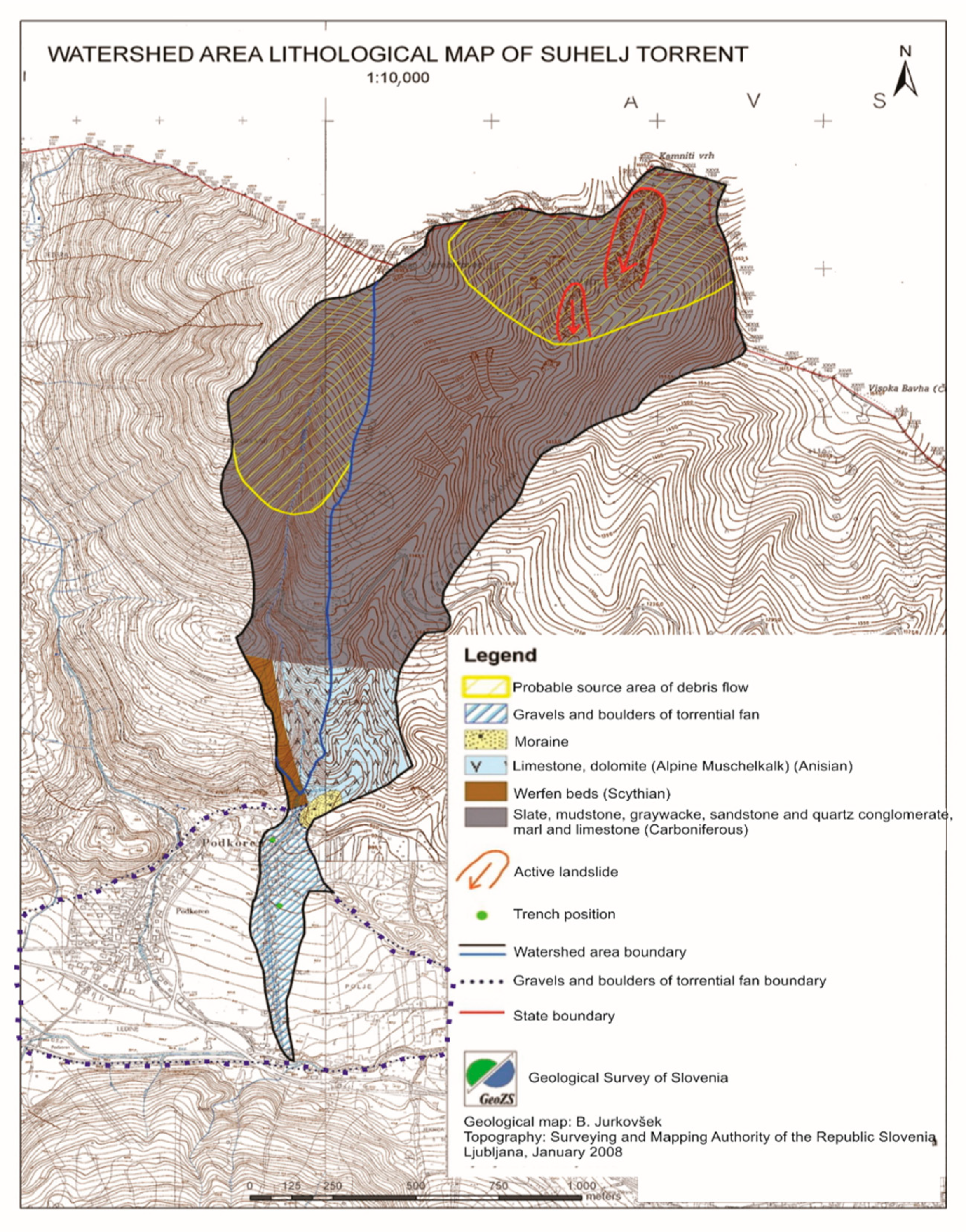
The Suhelj torrent is a part of the Upper Sava River (part of the Danube River basin), and it is located in north-west (NW) Slovenia (Figure 1) in the Western Karavanke mountain range [24]. Figure 2 shows a lithological map of the Suhelj torrent. The upper part of the catchment area is made of Lower Carbonifeorus rocks (slate, mudstone, greywacke, sandstone and quartz conglomerate, marl and limestone), and the lower part, including the torrential fan, is made of limestone and dolomite). In the uppermost part of the torrential catchment (close to the watershed and the border with Austria), there is large active sediment source yielding large quantities of fine-grained debris material to the Suhelj torrent (Figure 2). The sediment source was initiated in the years 1880–1890 as a large earth slump, and it has been estimated that up to now roughly 750,000 to 800,000 m3 of prevailing sandy–clayey sediments have been eroded from the source and transported downstream along the Suhelj torrent [25]. In the past, several check dams (the largest, 7 m high, is shown in Figure 3) were built in order to stabilize the channel bed and to capture debris flows and hyperconcentrated flows upstream of the populated Suhelj torrential fan. It should be noted that check dams are located upstream from the fan and thus do not impact on the simulation results.
Figure 4 shows the digital terrain model of the Suhelj fan that was used as an input to the RAMMS-DF model and the location of probing excavations on the Suhelj fan.
The Suhelj torrential catchment area is 1.9 km2, the average slope is 57%, and the average slope of the torrential fan is 11.8%. The average torrential channel slope is 16.9%, its length is 3.9 km, and the Melton number is 0.527 [26]. The Melton number can be calculated based on the topographic properties of the investigated catchment and can be used for the classification of fans (e.g., torrential, transitional, and debris-flow fans). Additional information about the Melton number can be found in, e.g., reference [26] and the references therein.
Hence, the Suhelj torrent is a typical torrential catchment where the topography can be characterized by steep slopes which yield short runoff times, and debris flows can occur in this area. Sodnik and Mikoš [26] classified the Suhelj torrential fan as debris-flow-prone area due to the fact that debris flows occurred in the past and because the Melton number and fan slope were higher than defined thresholds (i.e., Melton number higher than 0.3 and slope higher than 7%). Two probing excavations (Figure 4) 3.5 and 4 m deep, respectively, that exhibited 1–2 m thick layers of unconsolidated diamicts with the largest clasts of 10–20 cm [25] confirmed that debris flow occurred in the past.
Thus, the actual topography (a 4 m grid cell was used) could represent a good basis for the investigation of the impact of a random sequence of debris flows on the fan characteristics. For the Suhelj torrent, the officially available LIDAR data was used to represent the topography. For the Suhelj torrential fan case study, we used the input hydrograph option (the input hydrograph polygon is shown in Figure 4) because the RAMMS-DF manual suggests using a hydrograph for channelized debris flows and the block release option for open, un-channelized topographies [18].
2.3. Artificial Terrain
As a second case study, we defined an artificial terrain with a mild and constant slope (5°) (Figure 5). This slope was selected because debris fans often have similar characteristics (e.g., [26]). Furthermore, the Suhelj fan has a similar slope (i.e., ca. 7° as calculated in reference [26]). A block release option was used in this case study as suggested by the RAMMS-DF manual [18]. The release polygon was defined on the left part of the terrain with a constant slope of 5°. In order to minimize the cell size impact on the RAMMS model results, we also used 4 m grid cells for the artificial terrain (as for the Suhelj fan).
2.4. Debris-Flow Magnitudes and RAMMS-DF Parameters
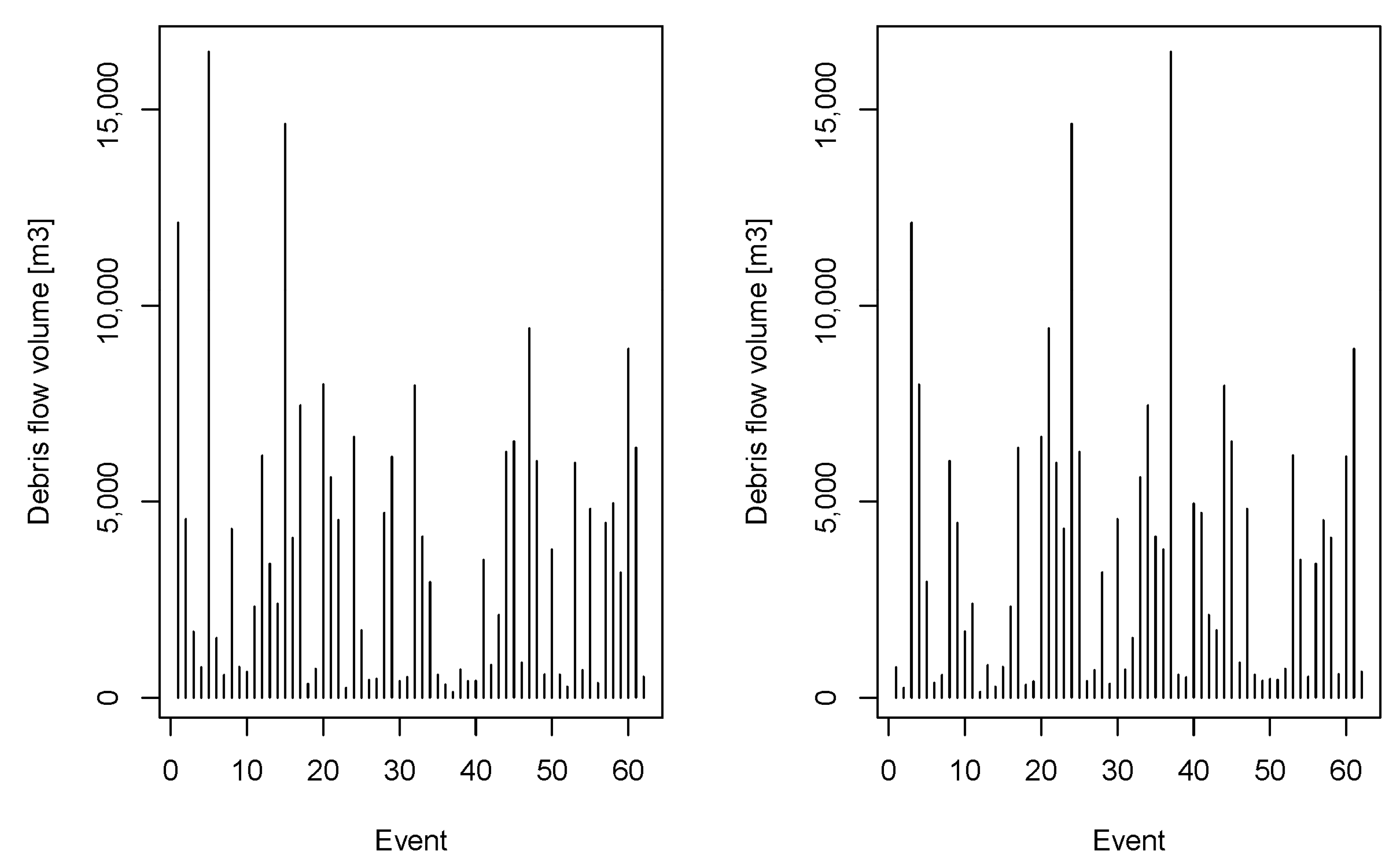
Due to lacking our own extensive database of historical debris flows on the Suhelj torrential fan, we tried to find good historical data in the Alpine environment with a rather long sequence of debris flows. Based on the study carried out by Stoffel [27], we defined the debris flow magnitudes that were used in this study. Stoffel investigated historical debris flow activity in a small catchment named Ritigraben (catchment area less than 5 km2) in Switzerland. Using tree-ring records and field surveys, Stoffel was able to estimate the magnitude of 62 debris flow events that occurred over about 150 years [27]. Stoffel classified debris flow magnitudes into four classes: S—small (25 events), M—medium (20 events), L—large (14 events), and XL—extra-large (3 events). Stoffel reported debris flow magnitudes as a range between a minimum and maximum value (e.g., for the S class, between 100 and 1000 m3). Because the literature about debris flow magnitudes is sparse and there are not many studies that have investigated the debris flow magnitude–frequency relationship (e.g., [28]), especially not in an environment similar to Slovenia (i.e., the Alps) we decided to adopt the magnitudes reported by Stoffel [27]. The only modification that was made compared to the previously mentioned study was that the maximum magnitude for the XL class was reduced from 5 × 10⁴ m3 to 2 × 10⁴ m3 based on the investigation performed by Sodnik and Mikoš [26]. For each class, the actual debris flow magnitudes were generated using a uniform distribution based on the minimum and maximum values of each class as defined by Stoffel [27]. The permutation was used to define the random sequence of debris flow events. Figure 6 shows an example of two different random sequences of the 62 investigated events. It should be noted that the total volume of debris flows (ca. 225,000 m3) was kept constant during simulations of different sequences.
For the Suhelj fan we adopted the triangular hydrograph shape with a total duration of 250 s where the peak was positioned 125 s after the start. For each model run, we changed the peak value based on the debris flow volume. For the artificial fan, the release depth was modified based on the debris flow volume and the block release area (polygon area).
One debris flow sequence included 62 model runs. After each RAMMS-DF run, the deposited material was added to the input topography, and this new topography was used in the next model run. The final fan after 62 events was used for further investigation. All model parameters were kept constant during all 62 model runs for the Suhelj fan and artificial terrain case studies (percentage of total momentum, 5%; dump step, 50 s; a second-order numerical scheme was used; density, 2000 kg/m3; lambda, 1; H cutoff, 0.000001 m; input angle did not change during the simulations). Based on the literature review (e.g., [10,11,12,13,18,29,30]), different sets of Voellmy parameters were used (Table 1). It should be noted that some of the cases shown in Table 1 could be regarded as unrealistic for the alpine environment (e.g., Cases 5–8). According to the literature (e.g., [10,11,12,13,18,29,30,31]), Cases 1 and 3 could perhaps be regarded as the most relevant for the selected case study (i.e., the Suhelj fan). However, we decided to also carry out simulations for other cases since these could be of interest for researchers dealing with other environments. For each of the eight parameter sets listed in Table 1, at least two random sequences were computed. The RAMMS modelling procedure (i.e., one sequence that was composed from 62 model runs) was performed automatically using a set of Autoit and R functions/scripts. This kind of combination was previously used for the automatic calibration of the Water and Tillage Erosion Model (WaTEM)/Sediment Delivery model (SEDEM) WaTEM/SEDEM model that can be used for soil erosion modelling [32].
2.5. Statistical t-Test and Mann–Whitney (MW) Test
For the comparison of fan characteristics, we used statistical t-tests and Mann–Whitney (MW) tests. Based on the maximum and minimum fan elevation after 62 RAMMS-DF runs, we counted the number of cells in different elevation classes (i.e., elevation difference from 0 to 0.4 m, from 0.4 m to 0.8 m, etc.). Only cells with an elevation difference larger than 1 cm were used. As an input to the t-test and MW test, we used the number of cells in all classes (log values were used in order to normalize the data). The t-test null hypothesis is that there is no difference between two tested groups (i.e., in our case, the elevation distribution after 62 model runs for different sequences of debris flows) and the alternative hypothesis states that there is a difference between two groups. Moreover, the MW test can be used to estimate whether two samples belong to the same distribution or are different in some way (e.g., mean, variance, skewness, or a combination of them) (e.g., [33]). A statistical significance level of 0.05 was used in this study. This means that if the calculated p-value is lower than 0.05, there exists a statistically significant difference between the two considered samples. Moreover, this would mean that the random sequence of debris flows has a significant impact on the fan characteristics. A calculated p-value higher than the selected significance level indicates that the random sequence of debris flows does not have a statistically significant impact on the fan characteristics. The R function t.test was used in this study to perform the t-test and calculate the p-values [34], and wilcox.test was used to compute the MW test [35].
3. Results and Discussion
3.1. Suhelj Fan
Figure 7 shows an example of modelling results for two random sequences for the µ = 0.1 and ξ = 100 Voellmy parameters. The final fan after the 62 RAMMS-DF model runs is shown. In order to investigate the random sequence’s impact on the fan, we compared the final elevation characteristics (i.e., elevation distribution) that are also shown in Figure 7. Table 2 shows the t-test and MW test p-values that were computed using the procedure described in Section 2.5. One can notice that all reported p-values are higher than the selected significance level of 0.05, which indicates that there is no statistical difference between the fan characteristics after 62 model runs using different sequences of debris flow events for all tested RAMMS-DF model parameters. Nevertheless, the differences between different debris flow sequences for the average and maximum fan height were up to 25% and 5%, respectively (Table 2). Moreover, the differences in the fan area were up to 30%, which indicates that there also exist differences between different sequences in terms of the amount of material that is transported outside of the selected calculation domain. Moreover, the amount of material that is transported outside the calculation domain can be up to around 30% of the total debris flow volume (i.e., 225,000 m3). However, we can assume that a larger calculation domain would not have a significant impact on the t-test and MW test results since there would probably be a higher number of cells with elevation difference up to a few centimeters (i.e., pink color cells shown in Figure 7). Moreover, one could argue that the parameters that were kept constant during the simulations that were carried out in the scope of this study could significantly affect fan characteristics. Such parameters are, for example, the percentage of total momentum (i.e., debris flow stop parameter), H cutoff, or input angle. We argue that if we were to randomly change these parameters during different debris flow events, we could, after 62 simulations, obtain results that would be significantly different from each other (e.g., for two sets of 62 model runs). Similarly, use of the erosion module that is available in RAMMS could affect the results since this is an important process that impacts on the debris flow volume. However, we did not use the erosion option in the simulations that are shown in this paper.
3.2. Artificial Terrain
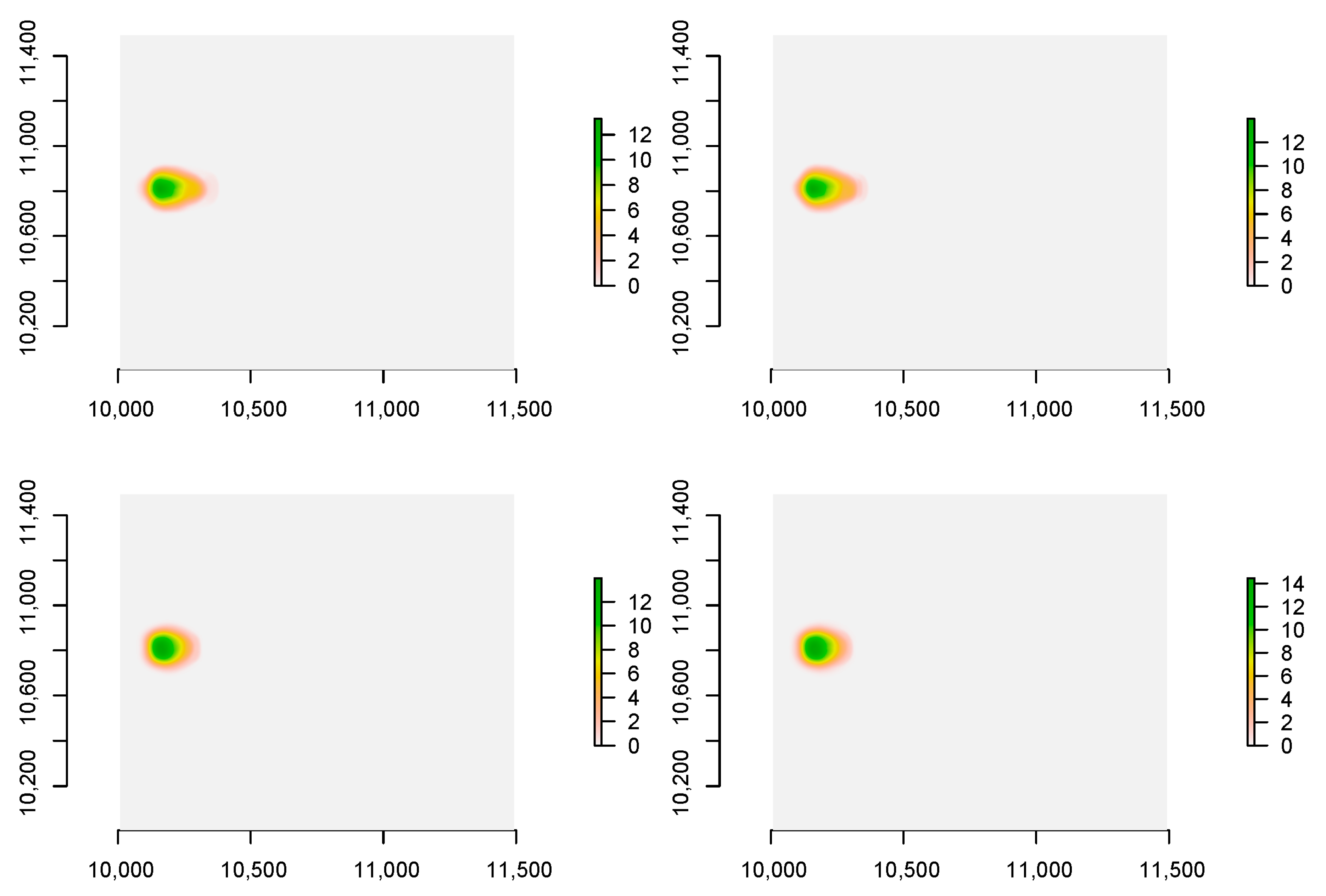
Figure 9 shows the fan after 62 model runs for different debris flow sequences for two parameter sets, namely, µ = 0.2 and ξ = 600 and µ = 0.4 and ξ = 100. As for the actual topography (i.e., the Suhelj fan), for the artificial terrain, the t-test and MW test p-values are higher than the selected significance level of 0.05 (Table 3). This again indicates that the sequence of debris flow events does not have a significant impact on the fan elevation distribution. Moreover, for the artificial terrain, the maximum differences between different sequences in terms of average and maximum fan height were up to 5%, which is less than the differences reported for the Suhelj fan case study. One can also notice that higher µ values (µ accounts for the resistance of the solid phase; [18]) yield higher fan heights (Table 2 and Table 3). This means that higher µ values also lead to higher fan slopes. The µ parameter dominates the debris flow movement when the flow is close to stopping [18]. On the other hand, the ξ parameter, which dominates the flow movement when the debris flow is running quickly [18], does not have a clear connection with the average and maximum fan heights (Table 2 and Table 3). More specifically, with increasing ξ parameter, the average and maximum fan heights are neither significantly decreasing nor increasing. Figure 10 shows differences among the investigated cases. One can notice that smaller µ, similarly as for the Suhelj case study, yielded smaller fan heights. However, compared to the Suhelj case study where we used actual terrain, one can notice that the impact of the µ parameter is obviously larger since the fan height is increasing with larger µ values. For the Suhelj fan (Figure 8), this increase was not so clear, which indicates that terrain characteristics have an important role in fan formation.
4. Conclusions
This paper presents results of an investigation into the impact of a random sequence of debris flows on torrential fan characteristics. Two case studies were selected, namely, an actual fan (the Suhelj fan) located in the NW of Slovenia and artificial terrain with a constant slope of 5°. Sixty-two debris flow events of different magnitudes (from 100 to 20,000 m3) represented one debris flow sequence. The permutation was used to determine different debris flow sequences. The final fan characteristics after 62 model runs were compared after RAMMS-DF was used for debris flow modelling. The elevation differences were compared using t-tests and MW tests. Several Voellmy model parameters were tested. Some of the tested cases (i.e., 1 and 3) can be regarded as more suitable for the alpine environment than others. The results indicate that the sequence of debris flow events does not have a statistically significant impact on the fan elevation distribution (at the selected significance level of 0.05). This conclusion was obtained for several tested model parameters and two different case studies, namely, the artificial terrain and actual debris fan. Some smaller differences were detected in the average and maximum fan heights. However, it seems that answer to the main scientific question stated in the introduction is that a random sequence of debris flows does not have a significant impact on the final fan characteristics. Moreover, further research is possible with the inclusion of other RAMMS parameters (e.g., input angle, percentage of total momentum) or some other kind of numerical experiment where the focus is on the fan formation. Furthermore, consideration of bed erosion in the RAMMS model could also be regarded as a potential future research step.
Author Contributions
All authors drafted the manuscript and determined the aims of the research; all authors contributed to the manuscript writing and its revision.
Funding
The results of the study are part of the research project J7-8273 “Recognition of potentially hazardous torrential fans using geomorphometric methods and simulating fan formation” that is financed by the Slovenian Research Agency (ARRS). This project was approved by the International Programme on Landslides (IPL) as the IPL-225 Project (http://iplhq.org/category/iplhq/ipl-ongoing-project/).
Conflicts of Interest
The authors declare no conflict of interest.
References
- Varnes, D.J. Landslide types and processes. In Landslides and Engineering Practice; Special Report 28; Eckel, E.B., Ed.; Highway Research Board, National Academy of Sciences: Washington, DC, USA, 1954; pp. 20–47. [Google Scholar]
- Varnes, D.J. Slope movement types and processes. In Landslides, Analysis and Control; Special Report 176; Schuster, R.L., Krizek, R.J., Eds.; Transportation Research Board. National Academy of Sciences: Washington, DC, USA, 1978; pp. 11–33. [Google Scholar]
- Hungr, O.; Leroueil, S.; Picarelli, L. The Varnes classification of landslide types, an update. Landslides 2015, 11, 167–194. [Google Scholar] [CrossRef]
- Jakob, M. Debris-flow hazard analysis. In Debris-Flow Hazards and Related Phenomena; Praxis; Jakob, M., Hungr, O., Eds.; Springer: Berlin/Heidelberg, Germany, 2005; pp. 411–443. [Google Scholar]
- Stoffel, M.; Bollschweiler, M.; Butler, D.R.; Luckman, B.H. (Eds.) Tree Rings and Natural Hazards—A State-of-the-Art; Springer Science+Business Media B.V: Dordrecht, The Netherlands, 2010; p. 505. [Google Scholar]
- Schneuwly-Bollschweiler, M.; Stoffel, M.; Rudolf-Miklau, F. (Eds.) Dating Torrential Processes on Fans and Cones—Methods and Their Application for Hazard and Risk Assessment; Springer Science+Business Media: Dordrecht, The Netherlands, 2013; p. 423. [Google Scholar]
- Rickenmann, D. Runout prediction methods. In Debris-Flow Hazards and Related Phenomena; Praxis; Jakob, M., Hungr, O., Eds.; Springer: Berlin/Heidelberg, Germany, 2005; pp. 305–324. [Google Scholar]
- Stancanelli, L.M.; Peres, D.J.; Cancelliere, A.; Foti, E. A combined triggering-propagation modeling approach for the assessment of rainfall induced debris flow susceptibility. J. Hydrol. 2017, 550, 130–143. [Google Scholar] [CrossRef]
- Christen, M.; Bühler, Y.; Bartelt, P.; Leine, R.; Glover, J.; Schweizer, A.; Graf, C.; Mc Ardell, B.W.; Gerber, W.; Deubelbeiss, Y.; et al. Integral hazard management using a unified software environment: Numerical simulation tool “RAMMS” for gravitational natural hazards. In Proceedings of the 12th Congress INTERPRAEVENT, Grenoble, France, 23–26 April 2012; Koboltschnig, G., Hübl, J., Braun, J., Eds.; pp. 77–86. [Google Scholar]
- Frank, F.; Mc Ardell, B.W.; Huggel, V.; Vieli, A. The importance of entrainment and bulking on debris flow runout modeling: Examples from the Swiss Alps. Nat. Hazards Earth Syst. Sci. 2015, 15, 2569–2583. [Google Scholar] [CrossRef]
- von Fischer, F.; Keiler, M.; Zimmermann, M. Modelling of individual debris flows using Flow-R: A case study in four Swiss torrents. In Proceedings of the INTERPRAEVENT 2016 Conference, Lucerne, Switzerland, 30 May–2 June 2016; pp. 257–264. Available online: http://www.interpraevent.at/palm-cms/upload_files/Publikationen/Tagungsbeitraege/2016_1_257.pdf (accessed on 22 January 2019).
- Frank, F.; Mc Ardell, B.W.; Oggier, N.; Baer, P.; Christen, M.; Vieli, A. Debris-flow modeling at Meretschibach and Bondasca catchments, Switzerland: Sensitivity testing of field-data-based entrainment model. Nat. Hazards Earth Syst. Sci. 2017, 17, 801–815. [Google Scholar] [CrossRef]
- Schraml, K.; Thomschitz, B.; McArdell, B.; Graf, C.; Kaitna, R. Modeling debris-flow runout patterns on two alpine fans with different dynamic simulation models. Nat. Hazards Earth Syst. Sci. 2015, 15, 1397–1425. [Google Scholar] [CrossRef]
- Vennari, C.; Mc Ardell, B.; Parise, M.; Santangelo, N.; Santo, A. Implementation of the RAMMS DEBRIS FLOW to Italian case studies. Geophys. Res. Abstr. 2016, 18, EGU2016-11378. [Google Scholar]
- Hussin, H.Y. Probabilsitic Run-out Modeling of a Debris Flow in Barcelonnette, France. Master’s Thesis, University of Twente, Enschede, The Netherlands, 2011; p. 94. Available online: https://webapps.itc.utwente.nl/librarywww/papers_2011/msc/aes/hussin.pdf (accessed on 22 January 2019).
- Hussin, H.Y.; Quan Luna, B.; van Westen, C.J.; Christen, M.; Malet, J.-P.; van Asch, T.W.J. Parameterization of a numerical 2-D debris flow model with entrainment: A case study of the Faucon catchment, Southern French Alps. Nat. Hazards Earth Syst. Sci. 2012, 12, 3075–3090. [Google Scholar] [CrossRef]
- Sherchan, B. Entrainment of Bed Sediments by Debris Flow. Master’s Thesis, Department of Civil and Transport Engineering, Norwegian University of Science and Technology, Trondheim, Norway, June 2016; p. 116. Available online: https://brage.bibsys.no/xmlui/bitstream/handle/11250/2416456/15278_FULLTEXT.pdf (accessed on 22 January 2019).
- RAMMS. User Manual v1.7.0 Debris Flow. 2018. Available online: http://ramms.slf.ch/ramms/downloads/RAMMS_DBF_Manual.pdf (accessed on 22 January 2019).
- Christen, M.; Kowalski, J.; Bartelt, P. RAMMS: Numerical simulation of dense snow avalanches in three-dimensional terrain. Cold Reg. Sci. Technol. 2010, 63, 1–14. [Google Scholar] [CrossRef] [Green Version]
- Christen, M.; Gerber, W.; Graf, C.; Bühler, Y.; Bartelt, P.; Glover, J.; Mc Ardell, B.; Feistl, T.; Steinkogler, W. Numerische Simulation von gravitativen Naturgefahren mit “RAMMS” (Rapid Mass Movements). Zeitschrift für Wildbach Lawinen Erosions und Steinschlagschutz 2012, 169, 282–293. [Google Scholar]
- Simoni, A.; Mammoliti, M.; Graf, C. Performance of 2D debris flow simulation model RAMMS. Back-analysis of field events in Italian Alps. In Proceedings of the Annual International Conference on Geological and Earth Sciences GEOS 2012, Singapore, 3–4 December 2012; p. 6. [Google Scholar]
- Grêt-Regamey, A.; Brunner, S.H.; Altwegg, J.; Christen, M.; Bebi, P. Integrating expert knowledge into mapping ecosystem services trade-offs for sustainable forest management. Ecol. Soc. 2013, 18, 34. [Google Scholar] [CrossRef]
- Hohermuth, B.; Graf, C. Einsatz numerischer Murgangsimulationen am Beispiel des integralen Schutzkonzepts Plattenbach Vitznau. Wasser Energ. Luft 2014, 106, 285–290. [Google Scholar]
- Mohorič, N.; Grigillo, D.; Jemec Auflič, M.; Mikoš, M.; Celarc, B. Longitudinal profiles of torrential channels in the Western Karavanke mountains. Geologija 2016, 59, 273–286. [Google Scholar] [CrossRef]
- UL FGG & GeoZS. Debris Flow Risk Assessment—Final Report; Faculty of Civil and Geodetic Engineering of the University of Ljubljana (UL FGG) & Geological Survey of Slovenia (GeoZS): Ljubljana, Slovenia, 2008; 224p, Available online: http://www.sos112.si/slo/tdocs/naloga_76.pdf (accessed on 22 January 2019). (In Slovenian)
- Sodnik, J.; Mikoš, M. Estimation of magnitudes of debris flows in selected torrential watersheds in Slovenia. Acta Geographica Slovenica 2006, 46, 93–123. [Google Scholar] [CrossRef] [Green Version]
- Stoffel, M. Magnitude–frequency relationships of debris flows—A case study based on field surveys and tree-ring records. Geomorphology 2010, 116, 67–76. [Google Scholar] [CrossRef]
- Johnson, P.A.; McCuen, R.H.; Hromadka, T.V. Magnitude and frequency of debris flows. J. Hydrol. 1991, 123, 69–82. [Google Scholar] [CrossRef]
- Cesca, M.; D’Agostino, V. Comparison between FLO-2D in RAMMS in debris-flow modelling: A case study in the Dolomites. WIT Trans. Eng. Sci. 2008, 60, 197–206. [Google Scholar]
- Scheuner, T.; Schwab, S.; McArdell, B. Appplication of a two-dimensional numerical model in risk and hazard assessment in Switzerland. In Proceedings of the 5th International Conference on Debris-Flow Hazards Mitigation: Mechanics, Prediction and Assessment, Padua, Italy, 14–17 June 2011. [Google Scholar]
- Quan Luna, B.; Cepeda, J.; Stumpf, S.; van Westen, C.J.; Remaitre, A.; Malet, J.P.; van Asch, T.W.J. Analysis and Uncertainty Quantification of Dynamic Run-Out Model Parameters for Landslides. In Landslide Science and Practice; Margottini, C., Canuti, P., Sassa, K., Eds.; Springer: Berlin/Heidelberg, Germany, 2013. [Google Scholar]
- Bezak, N.; Rusjan, S.; Petan, S.; Sodnik, J.; Mikoš, M. Estimation of soil loss by the WATEM/SEDEM model using an automatic parameter estimation procedure. Environ. Earth Sci. 2015, 74, 5245–5261. [Google Scholar] [CrossRef]
- Fagerland, M.W.; Sandvik, L. The Wilcoxon–Mann–Whitney test under scrutiny. Stat. Med. 2009, 28, 1487–1497. [Google Scholar] [CrossRef] [PubMed]
- R Software. Student’s t-Test. 2018. Available online: https://www.statmethods.net/stats/ttest.html (accessed on 22 January 2019).
- R Software. Wilcox Test. 2018. Available online: https://stat.ethz.ch/R-manual/R-devel/library/stats/html/wilcox.test.html (accessed on 22 January 2019).
Figure 1.
Location of the Suhelj fan in the north-west (NW) of Slovenia (Slovenia location: Long: 13.38°–16.61°; Lat: 45.42°–46.88°).
Figure 1.
Location of the Suhelj fan in the north-west (NW) of Slovenia (Slovenia location: Long: 13.38°–16.61°; Lat: 45.42°–46.88°).

Figure 2.
Lithological map of the Suhelj torrent (modified from [25]).
Figure 2.
Lithological map of the Suhelj torrent (modified from [25]).

Figure 3.
Seven-meter-high check dam in the middle section of the Suhelj torren (modified from [25]).
Figure 3.
Seven-meter-high check dam in the middle section of the Suhelj torren (modified from [25]).

Figure 4.
(a) Digital elevation model of the Suhelj torrential fan with indication of the input hydrograph location (orange polygon) used for the numerical simulation of fan formation by debris flows; (b) Locations of probing excavations on the Suhelj torrential fan (modified from [25])—green circles.

Figure 5.
Longitudinal cross section of the artificial terrain where the slope of the left part of the terrain is 5° and the right part is horizontal (slope 0°) (a) and a 3D presentation of the artificial terrain (b).
Figure 5.
Longitudinal cross section of the artificial terrain where the slope of the left part of the terrain is 5° and the right part is horizontal (slope 0°) (a) and a 3D presentation of the artificial terrain (b).

Figure 6.
Two examples of a random sequence of the 62 investigated debris flow events.

Figure 7.
Debris flow fan after 62 simulations for the Suhelj fan. The upper row shows results for µ = 0.1 and ξ = 100 (two random sequences; x and y axes are coordinates) and the lower row shows the distribution of elevation differences between fans after 62 simulations and the situation before simulations for cases shown in the upper row (only cells with differences larger than 1 cm are shown). Legends of the upper row figures represent total deposit thickness, and the unit is meters.
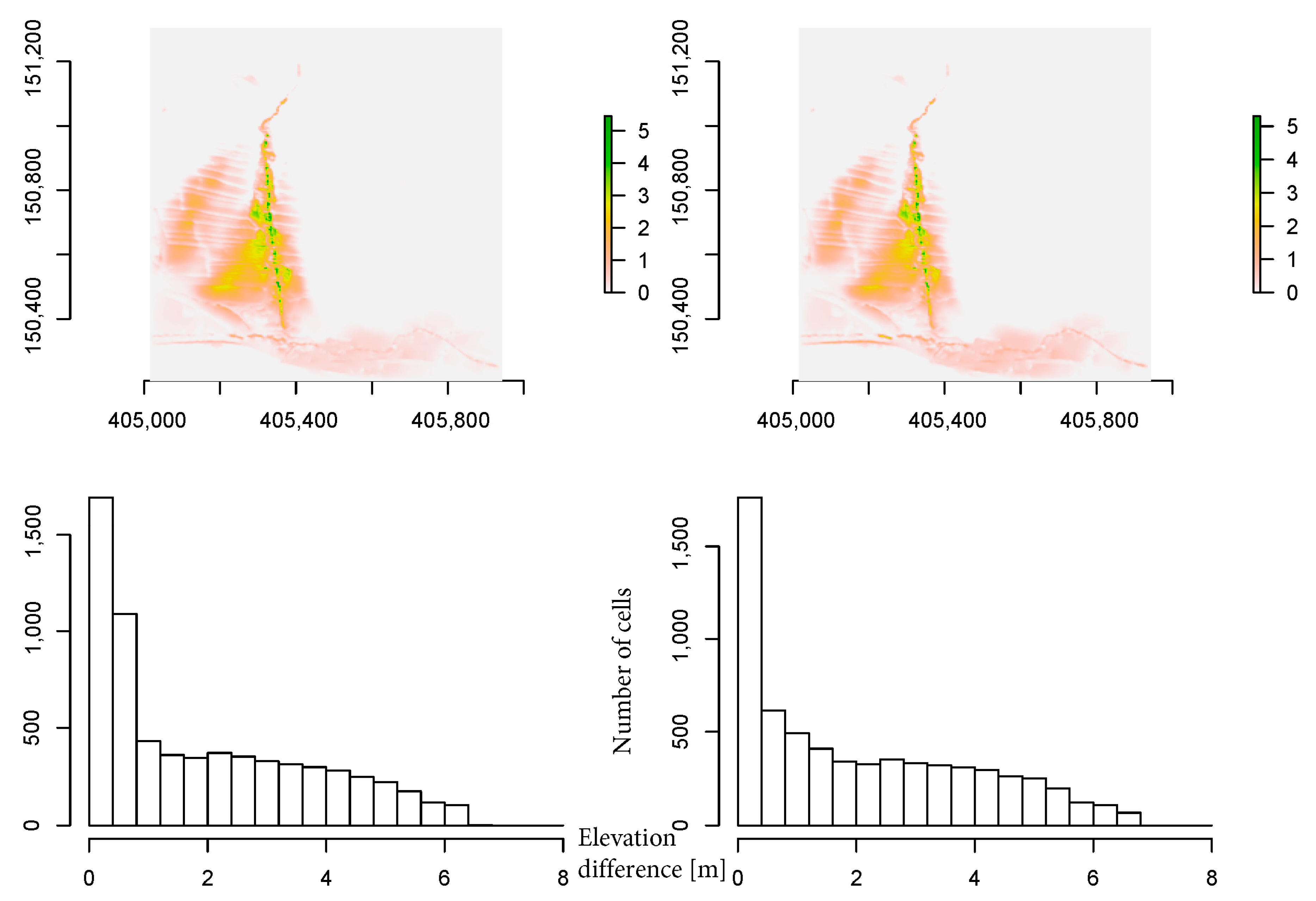
Figure 8.
Differences in the number of cells with specific height for all eight cases that are shown in Table 1 and that refer to different Voellmy parameters for the Suhelj fan area.
Figure 8.
Differences in the number of cells with specific height for all eight cases that are shown in Table 1 and that refer to different Voellmy parameters for the Suhelj fan area.

Figure 9.
Debris flow fans after 62 simulations for the artificial terrain. The upper row shows results for µ = 0.2 and ξ = 600 (two random sequences; x and y axes are coordinates) and the lower row shows results for µ = 0.4 and ξ = 100 (two random sequences). Legends of figures represent the total deposit thickness, and the unit is meters.

Figure 10.
Differences in the number of cells with specific height for all eight cases that are shown in Table 1 and that refer to different Voellmy parameters for the artificial terrain.
Figure 10.
Differences in the number of cells with specific height for all eight cases that are shown in Table 1 and that refer to different Voellmy parameters for the artificial terrain.


Table 1.
Voellmy parameters in the Rapid Mass Movement Simulations debris flow module (RAMMS-DF) model that were investigated in this study.
Table 1.
Voellmy parameters in the Rapid Mass Movement Simulations debris flow module (RAMMS-DF) model that were investigated in this study.
| Voellmy Parameters | Case Number |
|---|---|
| µ = 0.1, ξ = 100 ms−2 | 1 |
| µ = 0.1, ξ = 1500 ms−2 | 2 |
| µ = 0.2, ξ = 150 ms−2 | 3 |
| µ = 0.2, ξ = 600 ms−2 | 4 |
| µ = 0.4, ξ = 100 ms−2 | 5 |
| µ = 0.4, ξ = 400 ms−2 | 6 |
| µ = 0.4, ξ = 1500 ms−2 | 7 |
| µ = 0.5, ξ = 400 ms−2 | 8 |
Table 2.
Basic characteristics of the debris flow fan after 62 simulations for two random sequences of debris flow events for the Suhelj fan and t-test and MW test p-values. Average fan height was calculated using all cells that had more than 1 cm of deposited material.
Table 2.
Basic characteristics of the debris flow fan after 62 simulations for two random sequences of debris flow events for the Suhelj fan and t-test and MW test p-values. Average fan height was calculated using all cells that had more than 1 cm of deposited material.
| Case | Average Fan Height [m] | Maximum Fan Height [m] | Fan Area [ha] | Average Fan Height [m] | Maximum Fan Height [m] | Fan Area [ha] | t-test p-Value | MW test p-Value |
|---|---|---|---|---|---|---|---|---|
| 1 | 0.60 | 5.45 | 31.4 | 0.56 | 5.31 | 30.4 | 0.90 | 0.89 |
| 2 | 0.64 | 5.24 | 23.3 | 0.69 | 5.46 | 27.4 | 0.35 | 0.62 |
| 3 | 0.77 | 7.83 | 23.2 | 0.61 | 7.69 | 31.9 | 0.95 | 0.98 |
| 4 | 0.64 | 8.99 | 28.0 | 0.58 | 9.04 | 33.5 | 0.96 | 0.93 |
| 5 | 0.68 | 8.22 | 28.9 | 0.69 | 8.18 | 30.2 | 0.83 | 0.84 |
| 6 | 0.68 | 8.90 | 28.5 | 0.70 | 8.96 | 29.4 | 0.96 | 0.86 |
| 7 | 0.71 | 8.75 | 22.4 | 0.72 | 8.82 | 28.3 | 0.94 | 0.96 |
| 8 | 0.62 | 8.44 | 31.4 | 0.75 | 8.62 | 28.0 | 0.95 | 0.93 |
Table 3.
Basic characteristics of the debris flow fan after 62 simulations for two random sequences of debris flow events for the artificial terrain, and the t-test and MW test p-values. The average fan height was calculated using all cells that had more than 1 cm of deposited material.
Table 3.
Basic characteristics of the debris flow fan after 62 simulations for two random sequences of debris flow events for the artificial terrain, and the t-test and MW test p-values. The average fan height was calculated using all cells that had more than 1 cm of deposited material.
| Case | Average Fan Height [m] | Maximum Fan Height [m] | Fan Area [ha] | Average Fan Height [m] | Maximum Fan Height [m] | Fan Area [ha] | t-test p-value | MW test p-Value |
|---|---|---|---|---|---|---|---|---|
| 1 | 1.94 | 6.41 | 10.8 | 2.10 | 6.70 | 10.5 | 0.86 | 0.97 |
| 2 | 2.09 | 6.12 | 10.0 | 2.03 | 6.06 | 10.9 | 0.97 | 0.95 |
| 3 | 3.17 | 11.96 | 6.6 | 3.74 | 12.23 | 5.8 | 0.84 | 0.87 |
| 4 | 3.56 | 13.26 | 6.2 | 3.91 | 13.96 | 5.6 | 0.78 | 0.96 |
| 5 | 3.68 | 13.97 | 5.7 | 3.63 | 14.45 | 6.0 | 0.55 | 0.94 |
| 6 | 4.31 | 14.88 | 5.1 | 3.53 | 14.57 | 6.2 | 0.77 | 0.91 |
| 7 | 4.22 | 14.55 | 5.2 | 4.07 | 14.14 | 5.4 | 0.75 | 0.89 |
| 8 | 4.47 | 15.24 | 4.7 | 4.96 | 15.85 | 4.4 | 0.38 | 0.91 |
© 2019 by the authors. Licensee MDPI, Basel, Switzerland. This article is an open access article distributed under the terms and conditions of the Creative Commons Attribution (CC BY) license (http://creativecommons.org/licenses/by/4.0/).
Share and Cite
MDPI and ACS Style
Bezak, N.; Sodnik, J.; Mikoš, M. Impact of a Random Sequence of Debris Flows on Torrential Fan Formation. Geosciences 2019, 9, 64. https://doi.org/10.3390/geosciences9020064
AMA Style
Bezak N, Sodnik J, Mikoš M. Impact of a Random Sequence of Debris Flows on Torrential Fan Formation. Geosciences. 2019; 9(2):64. https://doi.org/10.3390/geosciences9020064
Chicago/Turabian StyleBezak, Nejc, Jošt Sodnik, and Matjaž Mikoš. 2019. "Impact of a Random Sequence of Debris Flows on Torrential Fan Formation" Geosciences 9, no. 2: 64. https://doi.org/10.3390/geosciences9020064
Note that from the first issue of 2016, this journal uses article numbers instead of page numbers. See further details here.