Interpolation of Small Datasets in the Sandstone Hydrocarbon Reservoirs, Case Study of the Sava Depression, Croatia

Abstract

The interpolation of small datasets is challenging problem regarding the selection of interpolation methods and type of datasets. Here, for such analysis, the analysed data was taken in two hydrocarbon fields (“A” and “B”), located in the western part of the Sava Depression (in Northern Croatia). The selected reservoirs “L” (in the “A” Field) and “K” (“B”) are of Lower Pontian (Upper Miocene) age and belong to the Kloštar-Ivanić Formation. Due to strong tectonics, there are numerous tectonic blocks, each sampled with only a few wells. We selected two variables for interpolation—reservoirs permeabilities and injected volumes of field water. The following interpolation methods are described, compared and applied: Nearest Neighbourhood, Natural Neighbour (for the first time in the Sava Depression) and Inverse Distance Weighting. The last one has been recommended as the most appropriate in this study. Also, the presented research can be repeated in similar clastic environments at the same level hydrocarbon of exploration.

1. Introduction

Mature hydrocarbon fields are often in the secondary or tertiary production phase. However, only the largest structures are well explored with numerous wells, testing, seismics, etc. The smaller ones, especially if they are divided into several tectonic blocks, can be considered as weakly explored subsurface volumes. In such cases, any recommendation how to present such a subsurface as reliably as possible is very useful for future production, exploration or injection. The analysed area of the Sava Depression (in Northern Croatia) is an example of a petroleum zone with numerous hydrocarbon fields, where many of them can be classified as faulted structural traps, divided in numerous blocks. In almost all fields secondary hydrocarbon recovery methods (water injection) have been applied since the 80s of the 20th century. Re-injection of formation water is the most widely used method of supporting formation pressure. Here fields “A” and “B” were analysed, where re-injection of field (formation) water was applied. Due to the relatively small hydrodynamic units, i.e., a small number of production and injection wells in such volumes, reservoir mapping can be done only by using simple interpolation methods. i.e., methods designed for a small number of input data, without complex spatial analysis (like Kriging/co-Kriging/simulations using a variogram or co-variance function).

Previous studies of the Miocene hydrocarbon reservoirs in the Sava Depression defined interpolation rules for datasets containing different numbers of measurement locations. According to [1,2] the minimum data for geostatistical mapping (Kriging) is set on 20 or more “hard” values, thus defining the boundary of the small input set. Also, [3,4] a set of 15 input data is defined as sufficient for the application of interpolation methods like Inverse Distance Weighting (abbr. IDW) and Nearest Neighbourhood (abbr. NN) in the Croatian part of the Pannonian Basin System (abbr. CPBS). Application of the IDW method in the CPBS was documented in the Beničanci and Stari Gradec Fields ([5,6,7]), both located in the Drava depression. The NN method was applied also in the Kloštar field ([8]), located in the Sava Depression. Moreover, [9] applied the IDW method on the Dardevey iron ore deposit (NE Iran), and compared it with the Ordinary Kriging technique. [10] compared the Ordinary Kriging with IDW on data from the East-Parvadeh coal deposit (Iran). [11] applied the IDW and calculated cross-validation for soil depth in the Medinipur Block area (West Bengal, India). [12] applied the IDW method to a small set of numbers (15 data) for groundwater levels in Sosnowica (West Polesie). [13] analysed the value of cross-validation for the six methods applied to climate data for Europe. [14] compared the IDW method with Simple and Ordinary Kriging for 3, 6, 12, and 24 data. Those examples presented applicability of such interpolations in similar problems of the subsurface spatial distributions. The three selected methods represent one of the most applied mathematically simpler interpolations in general. Two of them are linear estimators (IDW, NaN), where transition among values is represented with graded isolines. On contrary, one (NN) method is polygonal, where linearity has been replaced with single delineator line among values. The both approaches could have advantage and disadvantages regarding small datasets (20 points or less, based on previously interpolation analysis of hydrocarbon settings in the analysed subsurface).

Consequently, we applied the Nearest Neighbourhood, Inverse Distances Weighting and Natural Neighbour in the selected reservoir hydrodynamic unit. The goal was to obtain the highest possible quality of subsurface maps, and (despite regarding the relatively small number of data per reservoir variable) use them to support future water injection and production.

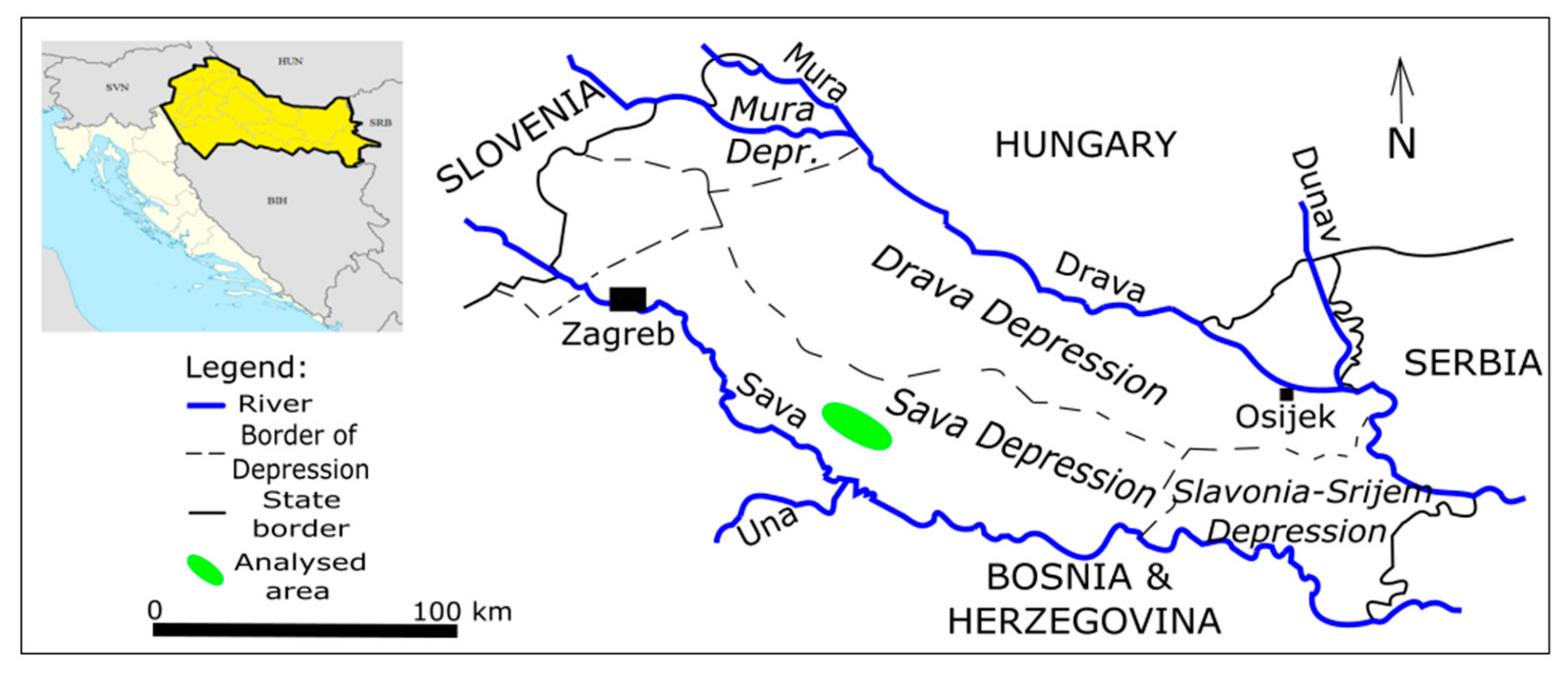
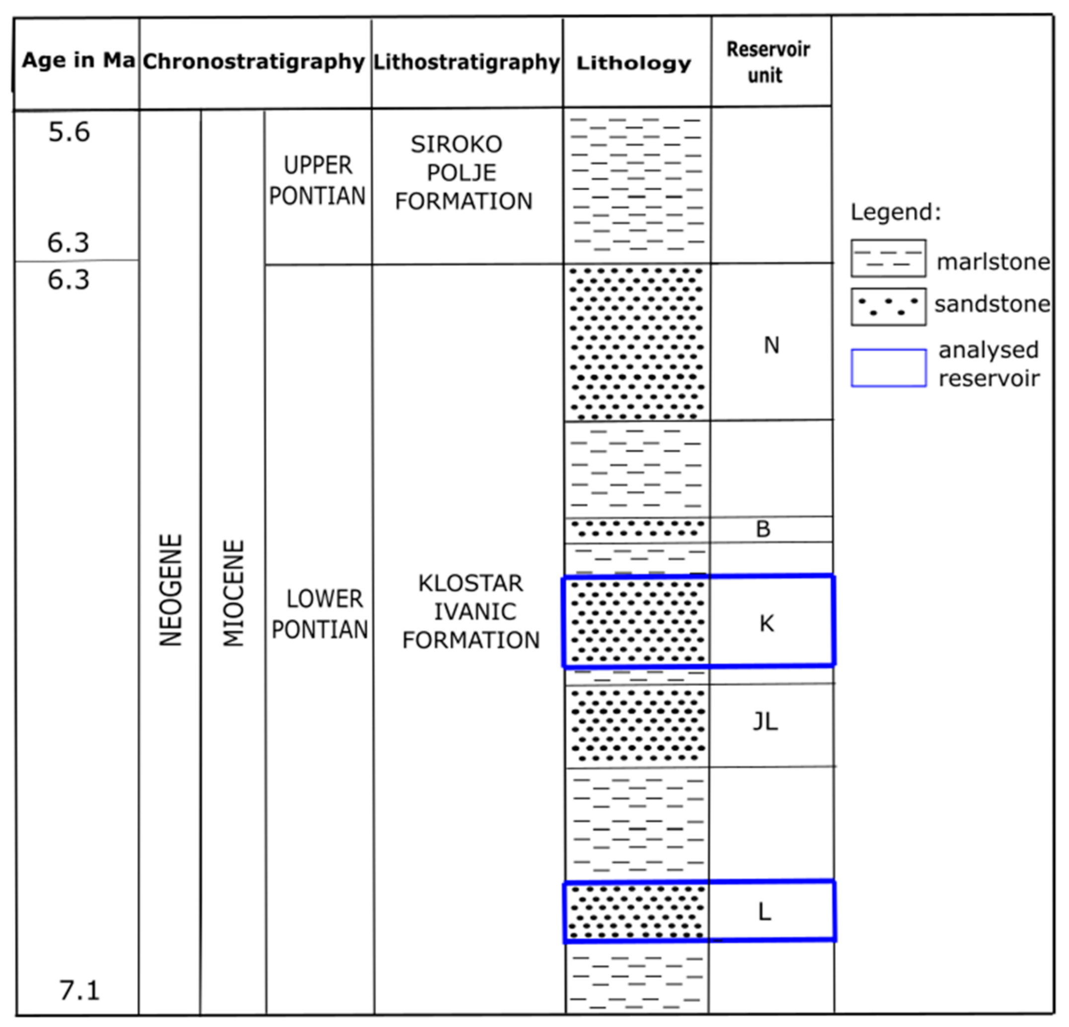
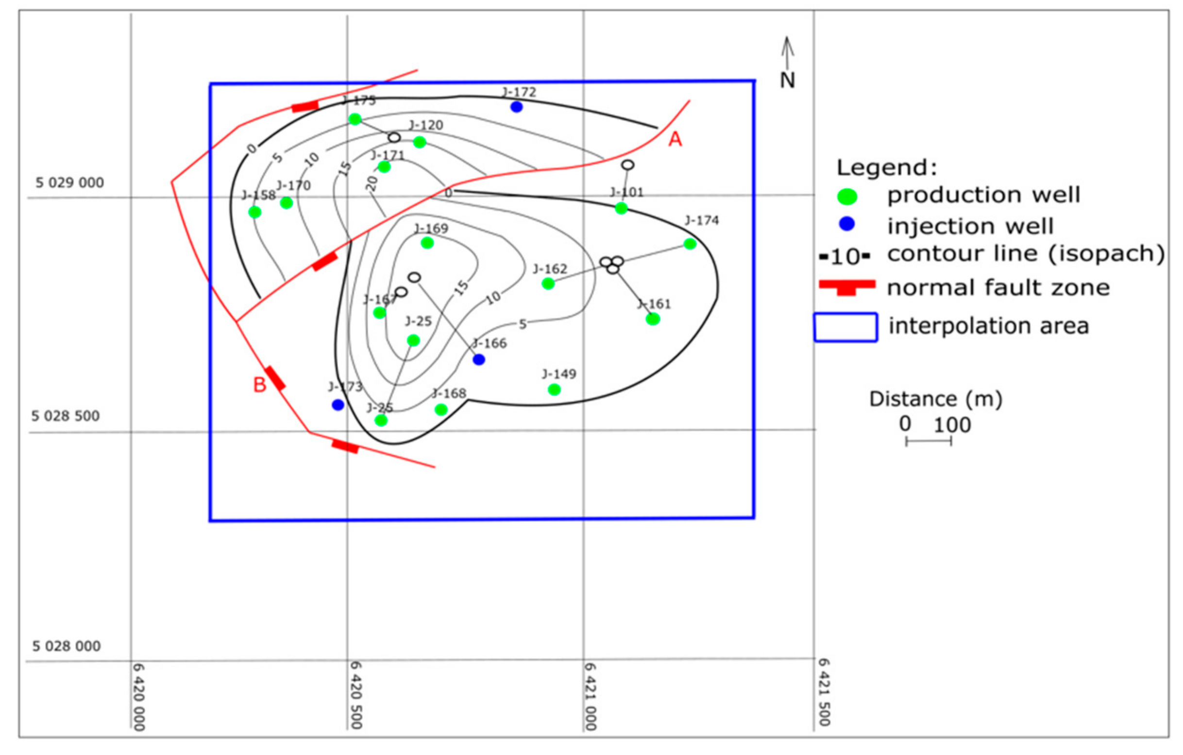
2. Geological Settings of the Sava Depression (Western Part)

Any interpolation of low-sampled hydrocarbon reservoirs depends on additional qualitative and quantitative data. The geological settings, particularly litho- and chronostratigraphic data, are standard part of such studies because they offer insight into depth, i.e., consolidation degree, and heterogeneity (or isotropy) of analysed lithology. Such data directly influence petrophysical and depended variables, like the porosity, permeability, saturation, injected volumes, effective reservoir thickness and recoverable reserves. Two such variable, permeability and injected volumes, has been analysed here.

The analysed “A” and “B” Fields are located in the CPBS, i.e., in the western part of the Sava Depression. They are located about 90 km southeast of the Croatian capital of Zagreb (see Figure 1).

Analysed reservoirs are of Lower Pontian age. Those are the “L” reservoir in the “A” and the “K” in the “B” Field. Lithostratigraphically, they are part of the Kloštar-Ivanić Formation (see Figure 2). The reservoir quality is briefly described with the following average values:

(a)

“L” reservoir—porosity 19.7%, horiz. permeability 17.5 × 10⁻³ µm² (17.5 mD), gross thickness 17.5 m;

(b)

“K” reservoir—porosity 22.7%, horiz. permeability 75.4 × 10⁻³ µm² (75.4 mD), gross thickness 10 m.

The entire area of the CPBS from the Late Pannonian until the Late Pontian period is considered as a dominant clastic environment, with enormously large volumes of sandy and silty detritus deposited from turbidites (e.g., [15]), which can be compared with provenance dataset at regional scale ([16,17]). The source areas were in the Eastern Alps, and detritus is transported toward the south-east, into the foothills by fluvial environments and, more distant into the lacustric environment of the Pannonian Lake. The transport was not continuous in one “moving event”, but periodical where large quantities were deposited at one of the numerous tectonic ramps in the basins and depressions of the SW margin of the PBS. One such structure was “the Legrad ramp” at the border between the Mura and Drava Depressions (see Figure 1). When these sediments reached gravitational instability, the detritus had been re-deposited toward the east (in the Drava Depression) or the south (in the Sava Depression).

Moreover, chronostratigraphically, many authors accepted Pontian as a valid stage in the entire Pannonian Basin System (e.g., [18,19,20]). However, recently some authors published some new depositional models of the Upper Miocene period that rejected the Pontian as a stage applied in the CPBS (e.g., [21]). In this analysis, the Pontian age has been used as valid unit for the description of reservoir stratigraphy, origin and age.

Hydrocarbon reservoirs described in Lower Pontian sandstones are of turbiditic origin. Their isolator rocks are marls, deposited during “calm” periods of pure lacustrine sedimentation.

A thickness map of the “L” reservoir is shown in Figure 3. We mapped the largest hydrodynamic unit where pressure is supported with water injection. The injection started in 1984 within 3 wells. Today such a process is maintained in 10 wells.

Figure 4 shows a thickness map of part of the “K” reservoir (“B” Field), i.e., hydrodynamic unit where the pressure is supported by re-injection of the formation water. The two largest hydrodynamic units (margined by faults in Figure 4) within the “K” reservoir have reserves accounting for about 50% of total hydrocarbons in the reservoir. That is why one of them is mapped in this analysis. The use of secondary hydrocarbon production methods has been applied since 1993 with a total of three injection wells.

3. Short Theory of Applied Interpolation Methods

Interpolation methods were described for mapping applied in the presented subsurface analyses. These are: Inverse Distance Weighting, Nearest Neighbourhood and Natural Neighbour. Their selection had been based on previous subsurface interpolation of numerous hydrocarbon reservoirs in the Sava Depression (e.g., [1,2,4,5]), where application of the geostatistics led to hardly interpretable results (e.g., [7]). There low number of hard-data prevented to calculate detailed spatial model using variogram function. Although all three selected methods are mathematically simple, there is need to present their equations and spatial interactions between measured and estimation points and make to reader simpler understand differences in results and interpretations among them.

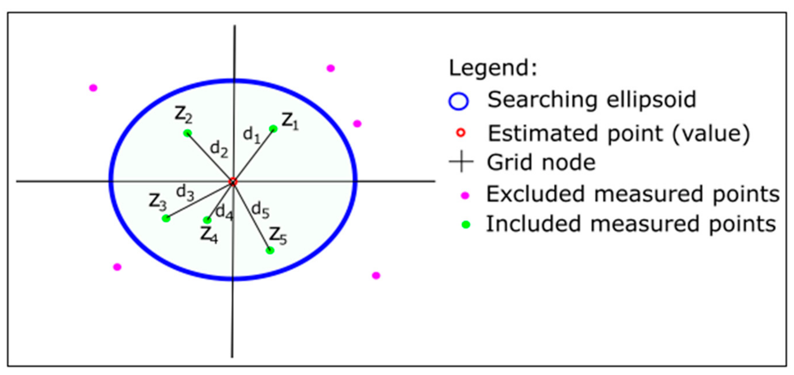
3.1. Inverse Distance Weighting Method

The Inverse Distance Weighting method is a mathematically simple interpolation method, where the unknown value of the variable is estimated from the measured values included into the searching circle (see Figure 5) or ellipsoid using Equation (1), based on a simple weighting method using the power of distances.

$${\mathrm{z}}_{\mathrm{iu}}=\frac{{{\displaystyle \sum }}_{i=1}^n\frac{{\mathrm{z}}_{\mathrm{i}}}{{\mathrm{d}}_{\mathrm{i}}^{\mathrm{p}}}}{{{\displaystyle \sum }}_{i=1}^n\frac{1}{{\mathrm{d}}_{\mathrm{i}}^{\mathrm{p}}}},$$

(1)

where: z_iu—estimated value; d_i—distance to “i-th” location; p—power of distance; z_i—measured values at “i-th” location.

The interpolation result depends exclusively on the distance, weighted by a power exponent that is commonly selected with values between 1 and 3. Usually in the subsurface of the CPBS, the value 2 is recommended, based on empirical tests performed in the subsurface geological mapping (e.g., [22,23]).

3.2. Nearest Neighbourhood Method

The Nearest Neighbourhood method is a simple interpolation method (see Figure 6) that adds a value to location E, taking into account the value of the nearest adjacent data (e.g., A, K, G, P on Figure 6), so the mapped area is covered by polygons (e.g., [24]).

Space distance is calculated according to the expression for Euclid’s distance (see Equation (2)), e.g., for points E and G, defined with coordinates in the Euclidean place (e₁, e₂) and (g₁, g₂), as:

$$d \left(E,G\right)= \sqrt{{(e_1-g_1)}^2+{(e_2-g_2)}^2},$$

(2)

where: d—distance; E and G—selected points (the closest ones) in space; e_i and g_i—coordinates of E and G in two dimensions.

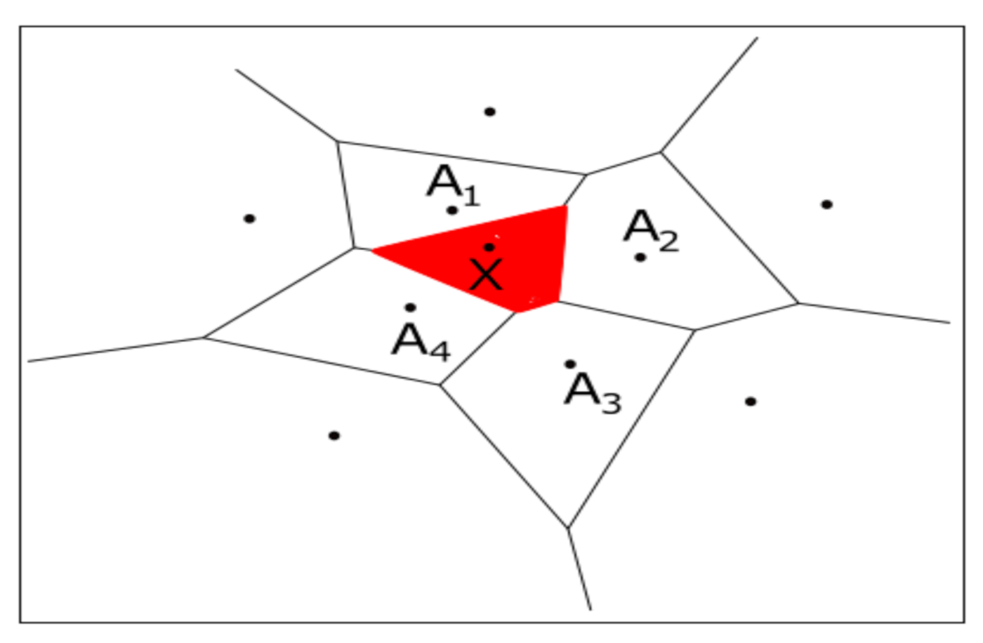
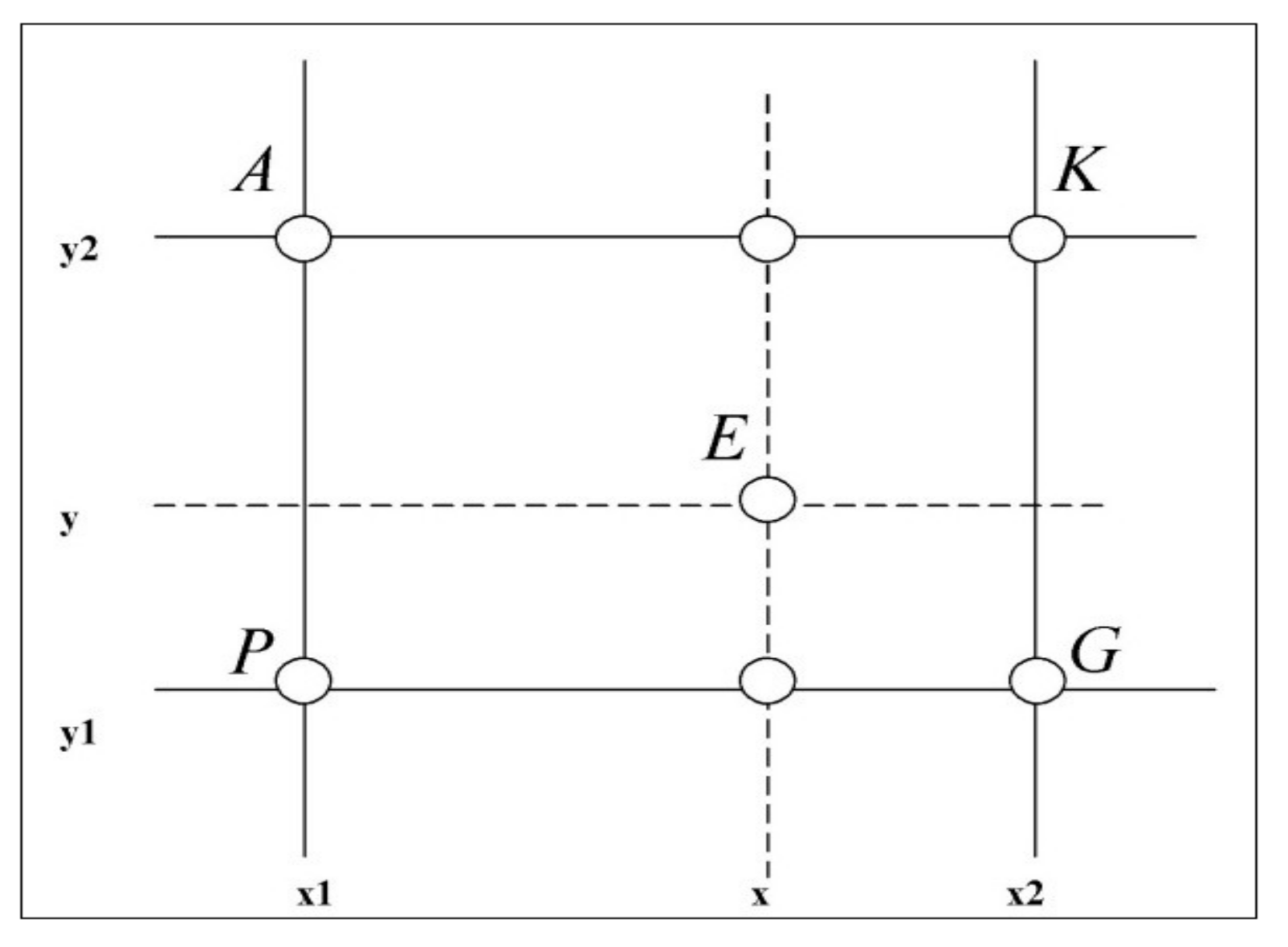
3.3. Natural Neighbour Method

The method of Natural Neighbour is a simple interpolation method based on Voronoi’s polygons. The unknown value “X” has been determined from, e.g., the four neighbouring values “A_1–4” as shown in Figure 7.

The mathematical expression for estimated Natural Neighbour values can be expressed with, e.g., Equation (3) (e.g., [25,26,27]):

$$X\left(x,y\right)={{\displaystyle \sum }}_{i=1}^n(w_{i}A\left(x_i,y_i\right),$$

(3)

where: X(x,y)—estimated point; A(x,y)—measured value in neighbouring points; w_i—proportion of analysed polygon regarding total area of all constructed adjacent polygons.

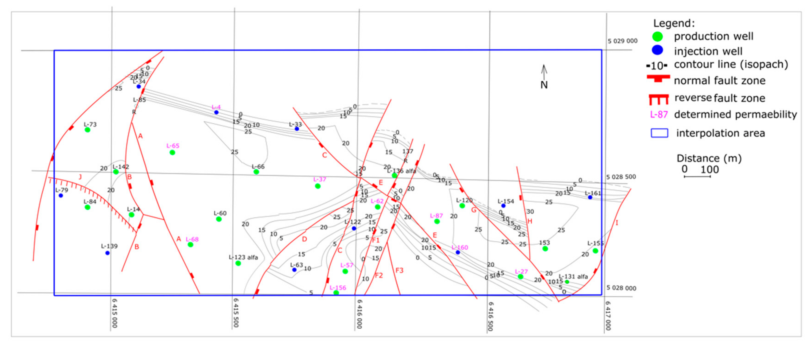
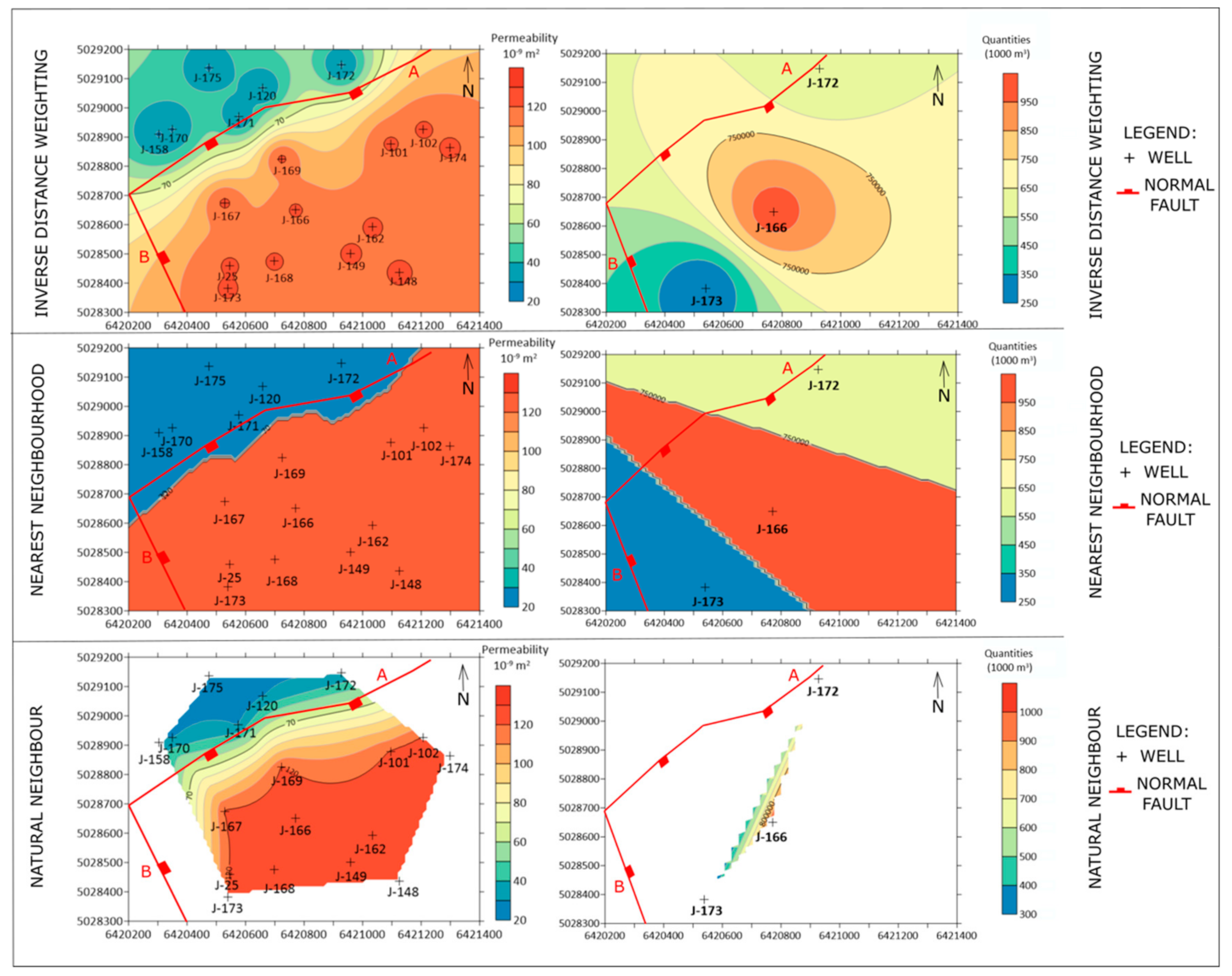
4. Interpolation in Reservoirs “L” and “K”—Injected Volumes and Permeabilities

The interpolated variables in both selected fields, were the permeability of the reservoir and the volumes of injected water. Those variables are crucial for the interpretation and planning of the secondary hydrocarbon recovery methods, i.e., field’s waters re-injection.

Permeabilities of reservoirs “L” and “K” are determined in wells from laboratory measurements and previously uniformly extrapolated in particular blocks.

Table 1. Averaged permeabilities and total injected volumes data in the “L” and “K” reservoirs.

Wells in Reservoir “L” (Average Value Belong to Each of These Wells)		Permeability (10−3 µm2) (Horiz. Averaged)
L-27, L-87, L-160		24.2
L-57, L-62, L-156		27.0
L-4, L-37, L-65, L-68		23.2
Wells in Reservoir “K” (Average Value Belongs to Each of These Wells)		Permeability (10−3 µm2) (Horiz. Averaged)
J-25, J-101, J-102, J-148, J-149, J-162, J-166, J-167, J-168, J-169, J-173, J-174		121.2
J-120, J-158, J-170, J-171, J-172, J-175		29.6
Reservoir “K”		Reservoir “L”
Well	Injected Volumes (m3)	Well	Injected Volumes (m3)
J-166	992,045	L-4	132,116
J-172	593,591	L-33	420,251
J-173	273,788	L-34	167,108
		L-63	440,031
		L-79	132,352
		L-122	535,171
		L-139	241,085
		L-154	565,872
		L-160	467,987
		L-161	376,438

shows the available data for permeability and injected volumes in the “L” and “K” reservoirs.

Interpolated maps in the “L” reservoir, using data from Table 1, has been shown in Figure 8 sequentially for all three methods—IDW, NN and NaN (from top to bottom). The cross-validation results are given in

Table 2. Cross-validation values for 3 methods and 2 variables in the “L” reservoir.

Variable	Number of Data	Values of Cross-Validation
		Inverse Distance Weighting	Nearest Neighbourhood	Natural Neighbour
Injected volumes	10	1.21 × 1010	2.64 × 1010	2.36 × 1010
Permeability	10	1.41	2.22	3.48

. These results are obtained with standard procedure when one measured value is omitted, and an estimation at the same location is calculated from the rest of the measured values. In this way, a second power of difference between real and estimated value is calculated for each location. Results are summed for all measured locations and are expressed as the value of cross-validation. This method is applied as the numerical test for quality if an estimation is performed with different methods, but with the same area (volume) and dataset.

The interpolation results for the same variables in the “K” reservoir are shown in Figure 9. The cross-validation results for applied interpolation methods are shown in

Table 3. Cross-validation values for 3 methods and 2 variables in the “K” reservoir.

Variable	Number of Data	Value of Cross-Validation
		Inverse Distance Weighting	Nearest Neighbourhood	Natural Neighbour
Injected volumes	3	2.86 × 1011	3.96 × 1011	-
Permeability	18	480.8	1397.4	1044.7

.

5. Discussion and Conclusions

Two interpolation (IDW, NaN) and one zonal (NN) method, as expected, gave different mapping results as well as cross-validation errors. But, interestingly, each of them led to at least one useful information about analysed reservoirs, i.e., about connection between permeability and injected water volumes, including the role of some fault zone. Here, the results of each particular method are given separately and brief recommendation has been given in

Table 4. Recommended interpolation methods for small input data set.

Number of Data	Applicability of Interpolation Method
	Inverse Distance Weighting	Nearest Neighbourhood	Natural Neighbour
1–5	Yes	Yes	No
6–10	Yes	Yes	Yes
11–19	Yes	Yes	Yes

.

The Inverse Distance Weighting maps showed a clear transitional zone, especially for the injected volumes variable. Such zones can somewhere be influenced by faults, e.g., such as the influenced permeability distribution in the “L” reservoir (see Figure 8, faults C, D, set of “F’s”), or in the “K” reservoir (see Figure 9, fault A). A similar situation can be observed for the injected volumes in Figure 8. Furthermore, the interpolation results for the “K” reservoir (see Figure 9, IDW, quantitates) clearly showed “bull’s-eye” or “butterfly” effects. Such features are usually observed in small datasets, and need to be carefully interpreted, neglected or re-calculated (e.g., [28]). A disadvantage of the IDW could be linear scaling applied in transition zones between two measured points. Regarding subsurface geology, it would be true only in a perfectly homogeneous reservoir, but real reservoirs are isotropic, even anisotropic, and often faulted.

The Nearest Neighbourhood maps are characterized with polygons (zones). That makes it possible to get quick insight in the general shape of the waterfront, but mostly in cases where the fault zones were impermeable (e.g., faults C, D, set of “F’s”, IDW, in Figure 8). Oppositely, the polygons can cross the fault zones (fault A, NN, Figure 9), which makes any interpretation very ambiguous, especially if fault permeability is uncertain. Another disadvantage is the absence of a transition zone between individual wells, which can be a problem in cases of small numbers of wells/polygons (quantities, Figure 9). Obviously, the polygonal method eliminated the “bull’s-eye” effect, but also offered a very interesting interpretation of the fault role. It is clear that fault A (see Figure 9) influenced the permeability distribution, i.e., was older than the reservoir, but obviously, the fault did not define the waterfront, at least as it can be interpreted with the IDW and NN maps. The similar situation can be observed in Figure 8 (faults C, D, F’s; IDW, NN), where most of them partially defined the borders of the permeability polygons, but not the firm borders of injected volumes.

The Natural Neighbour has one crucial difference. The method does not use extrapolation, i.e., interpolation has been done among the marginal points (see Figure 8 and Figure 9). Inside the interpolation area it uses transitional plotting, like the IDW. Generally, the method is unusable for datasets with approx. less than 5 points, because the interpolated area is too small compared with the margins of the selected area (reservoir, hydrodynamic unit or similar).

Regarding analysed variables, the cumulative volumes of injected water, and indirectly the moving of the water front, can be followed most easily with the IDW maps (see Figure 8 and Figure 9). Polygonal methods, in case of only two points, do not work, which is seen in Figure 9 (2nd row-right, NN, quantities) where two adjacent wells like J-166 and J-173 wells are separated with a line, which is not possible in relatively isotropic sandstone reservoirs at distances lower than 400 m. Based on production history, i.e., empirically as values used for different professional field’s works, the transitional zones, are defined as areas where the differences of injected volumes in two adjacent wells is larger than 50,000 m³.

All given examples are maps interpolated with small datasets, defined as a set with less than 20 points that cannot be spatially analysed with advanced methods like Kriging. The Kriged maps can be reliable obtained for, approx., datasets of 20 or more data, i.e., for any datasets where it is possible to calculate a reliable variogram or co-variance) model(s). Moreover, the analysed dataset has been divided into three classes: (a) 1–5, (b) 6–10 and (c) 11–19 points. Class (a) cannot be analysed with the NaN method because it is often not possible to calculate the cross-validation and the interpolated area is very small regarding unit margins. For class (b), all three methods can give results, as well as in class (c). The main selection criteria could be cross-validation. In all the cases, the IDW had the smallest value (see Table 2 and Table 3). However, this method sometimes created inside transitional zones numerous “bull’s-eyes” or “half-butterfly” features. The applicability of the tested method is summarised in the Table 4.

Analysed reservoirs can be mapped using the IDW, for any volume or area that includes less than 20 points (of “hard” data). However, if IDW maps show a large number of “bull’s-eyes” or “butterfly” features, it is recommended to additionally perform the NN, compare results in such zones and jointly interpret (such as the comparison done for the results of three methods in Figure 8 and Figure 9).

As final note, the reader needs to take into consideration that here are (intentionally) analysed two the most stochastic reservoir variables, e.g., permeability and (especially) injected water volumes. They are selected with purpose to make some kind of sensitivity analysis. As we reached interpretable results, the last statement is that applied analysis would be, for sure, useful for the more “isotropic” reservoir variables like porosity and thickness.

References

1. Malvić, T. History of geostatistical analyses performed in the Croatian part of the Pannonian Basin System. Nafta 2012, 63, 223–235. [Google Scholar]
2. Mesić Kiš, I.; Malvić, T. Zonal estimation and interpolation as simultaneous Approaches in the case of small input data set (Šandrovac Field, Northern Croatia). Min. Geol. Pet. Eng. Bull. 2014, 29, 9–16. [Google Scholar]
3. Novak Zelenika, K.; Cvetković, M.; Malvić, T.; Velić, J.; Sremac, J. Sequential Indicator Simulations maps of porosity, depth and thickness of Miocene clastic sediments in the Kloštar field, Northern Croatia. J. Maps 2013, 9, 550–557. [Google Scholar] [CrossRef]
4. Husanović, E.; Malvić, T. Review of deterministic geostatistical mapping methods in Croatian hydrocarbon reservoirs and advantages of such approach. Nafta 2014, 65, 57–63. [Google Scholar]
5. Malvić, T.; Đureković, M. Application of methods: Inverse distance weighting, ordinary kriging and collocated cokriging in porosity evaluation, and comparison of results on the Beničanci and Stari Gradac fields in Croatia. Nafta 2003, 54, 331–340. [Google Scholar]
6. Smoljanović, S.; Malvić, T. Improvements in reservoir characterization applying geostatistical modelling (estimation & stochastic simulations vs. standard interpolation methods), Case study from Croatia. Nafta 2005, 56, 57–63. [Google Scholar]
7. Malvić, T. Primjena Geostatistike u Analizi geoloških Podataka (Application of Geostatistics in Geological Data Analysis); INA-Industrija nafte d.d.: Zagreb, Croatia, 2008. [Google Scholar]
8. Balić, D.; Velić, J.; Malvić, T. Selection of the most appropriate interpolation method for sandstone reservoirs in the Kloštar oil and gas field. Geol. Croat. 2008, 61, 27–35. [Google Scholar]
9. Shahbeik, S.; Afzal, P.; Moarefvand, P.; Qumarsy, M. Comparison between ordinary kriging (OK) and inverse distance weighted (IDW) based on estimation error. Case study: Dardevey iron ore deposit, NE Iran. Arab. J. Geosci. 2014, 7, 3693–3704. [Google Scholar]
10. Afzal, P. Comparing ordinary kriging and advanced inverse distance squared methods based on estimating coal deposits; case study: East-Parvadeh deposit, central Iran. J. Min. Environ. 2018, 9, 753–760. [Google Scholar]
11. Bhunia, G.S.; Shit, P.K.; Maiti, R. Comparison of GIS-based interpolation methods for spatial distribution of soil organic carbon (SOC). J. Saudi Soc. Agric. Sci. 2016, 17, 114–126. [Google Scholar] [CrossRef]
12. Kamińska, A.; Grzywna, A. Comparison of deteministic interpolation methods for the estimation of groundwater level. J. Ecol. Eng. 2014, 15, 55–60. [Google Scholar]
13. Hofstra, N.; Haylock, M.; New, M.; Jones, P.; Frei, C. Comparison of six methods for the interpolation of daily European climate data. J. Geophys. Res. 2008, 113, 1–19. [Google Scholar] [CrossRef]
14. Babak, O.; Clayton, V.D. Statistical approach to inverse distance interpolation. Stoch. Environ. Res. Risk Assess. 2008, 23, 543–553. [Google Scholar] [CrossRef]
15. Malvić, T. Review of Miocene shallow marine and lacustrine depositional environments in Northern Croatia. Geol. Q. 2012, 56, 493–504. [Google Scholar] [CrossRef]
16. Critelli, S. Provenenace of Mesozoic to Cenozoic circum-Mediterranean sandstones in relation to tectonic setting. Earth Sci. Rev. 2018, 185, 624–648. [Google Scholar] [CrossRef]
17. Critelli, S.; Muto, F.; Perri, F.; Tripodi, V. Interpreting Provenance Relations from Sandstone Detrital Modes, Southern Italy Foreland Region: Stratigraphic record of the Miocene tectonic evolution. Mar. Pet. Geol. 2017, 87, 47–59. [Google Scholar] [CrossRef]
18. Popov, S.V.; Rogl, F.; Rozanov, A.Y.; Steininger, F.F.; Shcherba, I.G.; Kovac, M. Lithological-Paleogeographic maps of Paratethys 10 maps Late Eocene to Pliocene. Cour. Forsch. Senckenberg 2004, 250, 1–46. [Google Scholar]
19. Popov, S.V.; Shcherba, I.G.; Ilyina, L.B.; Nevesskaya, L.A.; Paramonova, N.P.; Khondkarian, S.O.; Magyar, I. Late Miocene to Pliocene palaeogeography of the Paratethys and its relation to the Mediterranean. Palaeogeogr. Palaeoclimatol. Palaeoecol. 2006, 238, 91–106. [Google Scholar] [CrossRef]
20. Piller, W.E.; Harzhauser, M.; Mandic, O. Miocene Central Paratethys stratigraphy– current status and future directions. Stratigraphy 2007, 4, 151–168. [Google Scholar]
21. Pavelić, D.; Kovačić, M. Sedimentology and stratigraphy of the Neogene rift-type North Croatian Basin (Pannonian Basin System, Croatia): A review. Mar. Pet. Geol. 2018, 91, 455–469. [Google Scholar] [CrossRef]
22. Malvić, T. Kriging, cokriging or stochastical simulations, and the choice between deterministic or sequential approaches. Geol. Croat. 2008, 61, 37–47. [Google Scholar]
23. Ivšinović, J. Deep mapping of hydrocarbon reservoirs in the case of a small number of data on the example of the Lower Pontian reservoirs of the western part of Sava Depression. In Proceedings of the 2nd Croatian congress on geomathematics and geological terminology, Zagreb, Croatia, 6 October 2018. [Google Scholar]
24. Olivier, R.; Hanqiang, C. Nearest Neighbor Value Interpolation. Int. J. Adv. Comput. Sci. Appl. 2012, 3, 18–24. [Google Scholar] [CrossRef]
25. Boissonnat, J.-D.; Cazals, F. Natural neighbor coordinates of points on a surface. Comput. Geom. 2001, 19, 155–173. [Google Scholar] [CrossRef]
26. Tsidaev, A. Parallel Algorithm for Natural Neighbor Interpolation. In Proceedings of the 2nd Ural Workshop on Parallel, Distributed, and Cloud Computing for Young Scientists, Yekaterinburg, Russia, 6 October 2016. [Google Scholar]
27. Traversoni, L. Natural neighbour finite elements. Trans. Ecol. Environ. 1994, 8, 291–297. [Google Scholar]
28. Malvić, T.; Ivšinović, J.; Velić, J.; Rajić, R. Kriging with a Small Number of Data Points Supported by Jack-Knifing, a Case Study in the Sava Depression (Northern Croatia). Geosciences 2019, 9, 36. [Google Scholar] [CrossRef]
Figure 1. Geographic position of “A” and “B” Fields within the Sava depression (in Northern Croatia).
Geosciences 09 00201 g001
Figure 2. Typical geological column for the western part of the Sava Depression, with (litho + chrono) stratigraphic positions of analysed reservoirs (“L” in “A” Field, “K” in “B” Field).
Geosciences 09 00201 g002
Figure 3. Thickness (isopach) map of the reservoir “L”, with borders of interpolated area, fault zone and (injection and production) wells.
Geosciences 09 00201 g003
Figure 4. Thickness (isopach) map of the reservoir “K”, with borders of interpolated area, fault zone and (injection and production) wells.
Geosciences 09 00201 g004
Figure 5. Searching ellipsoid, measured and estimated points used for the Inverse Distance Weighting calculation.
Geosciences 09 00201 g005
Figure 6. Nearest Neighbourhood grid where estimation in E is done regarding to points A, K, P or G (e.g., [24]).
Geosciences 09 00201 g006
Figure 7. Nearest Neighbour grid where estimation in the X is done regarding to points A1–A4 (e.g., [25,26]).
Geosciences 09 00201 g007
Figure 8. Results of IDW, NN and NaN methods (from top to bottom) of the permeability (left) and injected volumes (right) in the “L” reservoir. Faults are marked with letters, as are mentioned in the text.
Geosciences 09 00201 g008
Figure 9. Results of IDW, NN and NaN methods (from top to bottom) of the permeability (left) and injected volumes (right) in the “K” reservoir. Faults are marked with letters, as mentioned in the text.
Geosciences 09 00201 g009