Abstract
To estimate the potential inventory of natural gas hydrates (NGH) in the Levant Basin, southeastern Mediterranean Sea, we correlated the gas hydrate stability zone (GHSZ), modeled with local thermodynamic parameters, with seismic indicators of gas. A compilation of the oceanographic measurements defines the >1 km deep water temperature and salinity to 13.8 °C and 38.8‰ respectively, predicting the top GHSZ at a water depth of ~1250 m. Assuming sub-seafloor hydrostatic pore-pressure, water-body salinity, and geothermal gradients ranging between 20 to 28.5 °C/km, yields a useful first-order GHSZ approximation. Our model predicts that the entire northwestern half of the Levant seafloor lies within the GHSZ, with a median sub-seafloor thickness of ~150 m. High amplitude seismic reflectivity (HASR), correlates with the active seafloor gas seepage and is distributed across the deep-sea fan of the Nile within the Levant Basin. Trends observed in the distribution of the HASR are suggested to represent: (1) Shallow gas and possibly hydrates within buried channel-lobe systems 25 to 100 mbsf; and (2) a regionally discontinuous bottom simulating reflection (BSR) broadly matching the modeled base of GHSZ. We therefore estimate the potential methane hydrates resources within the Levant Basin at ~100 trillion cubic feet (Tcf) and its carbon content at ~1.5 gigatonnes.
1. Introduction
Gas hydrates are non-stoichiometric crystalline solids that are formed under a suitable thermodynamic pressure–temperature–salinity balance of water molecules, arranged in lattice-like crystal “cages” around gas molecules (e.g., [1,2]). Natural gas hydrates (NGH) deposits are widely distributed along the continental margins around the world, where gas fluxes are steadily available in the shallow sediment [2,3,4,5,6,7]. Their presence is bound in the marine environment between the top of the gas hydrate stability zone (GHSZ) in the water column, and its base within the sedimentary column below the seafloor. These are set by a thermodynamic balance between the impacts of pressure, temperature, and salinity on the hydrate stability [8]. In practice, the GHSZ is primarily controlled by the balance between the increase of water and sediment pressure with depth, the bottom water temperature and the increase in temperature with the depth beneath the seafloor. In many places, the presence of NGH is marked on seismic images by a bottom simulating reflection (BSR), suggested to represent the accumulation of free gas below the GHSZ [9,10,11]. However, NGH are also reported in areas without the presence of a distinct BSR (e.g., [12,13,14]), and a seismic BSR does not always indicate the presence of NGH (e.g., [14,15]).
NGH are estimated to contain a substantial portion of all organic carbon on Earth, and therefore play a crucial role in the global carbon cycle [2,16,17] and constitute a major potential energy resource [18]. Moreover, the precarious stability of NGH may lead to their dissociation in response to global warming. This may release vast amount of methane gas, which would induce a positive climate warming feedback [1,19,20,21,22]. Alternatively, dissociation may occur locally in the course of offshore activities, constituting a significant geohazard [23,24].
Isolated from the buffering effects of the global oceanic system, the Eastern Mediterranean Sea (EMS; Figure 1) is particularly sensitive to global climate changes [24,25,26,27]. With a major part of its seafloor within the GHSZ [28,29], this region would be expected to sustain a significant NGH potential [5,30,31]. Thus, global and regional changes would be expected to result in accentuated dissociation of hydrates in the EMS, which might result in a prominent climatic feedback response. In addition, the EMS can offer a relatively closed-system natural laboratory to study the linkage between environmental changes and NGH stability (e.g., [29]). Moreover, ongoing deep-sea discovery and development of prominent natural gas reservoirs across the southeastern Mediterranean Sea, and particularly in the Levant Basin (Figure 1) [32], invoke the need for addressing the possible presence of NGH in this area. However, across the entire EMS region, NGH were recovered to date only in a few mud volcanoes, and in spite of the pervasive exploration of the region no additional verified presence of hydrates was observed [33].
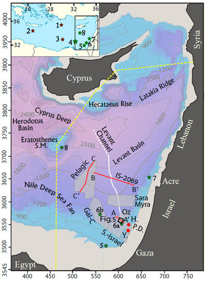
Figure 1.
A color-coded and contoured bathymetric map of the Levant Basin [62], overlaid with the outlines of the 3D seismic blocks (gray areas) and the TGS IS-2069 seismic profile (gray line) analyzed in this work. The outlines of the seismic traverses displayed in Figures 6–8 are marked (red lines) and labeled. Also marked are the locations of Hanna (H.) and Yam (Y.) wells (red dots), the outline of Figure 5 (black rectangle), and the northern and western border of the study area (yellow dashed line). The inset (upper left corner) displays a map of the Eastern Mediterranean Sea (EMS), marked with natural gas hydrates (NGH) (brown stars) and methane seepage (green stars) observations locations: 1. The Thessaloniki mud volcano and Anaximander Seamount region (e.g., [33,63,64]); 2. the Olimpi mud volcanos field (e.g., [33], and references therein); 3. observations of hydrates formation during sampling [65]; 4. the Nile Delta and deep sea fan seepage domain (e.g., [66,67]); 5. seafloor seepage offshore the Sinai Peninsula [68]; 6. (a) the Palmahim disturbance (P.D.) and Levant Channel (white line), and (b) Gal-C, seepage sites [69,70,71]; 7. methane sampling offshore acre [70]; 8. Eratosthenes Seamount seepage sites [72,73]. The main map is plotted in UTM coordinates (zone 36N, datum WGS84) and labeled in km, while the inset is plotted in geographical coordinates.
This study re-assesses the potential presence of NGH in the Levant Basin (Figure 1) through focused modeling of the GHSZ in the region and examining its correlation with a set of new observations. The results of this study are expected to serve as a base for future evaluation of the controls and possible impact of such presence.
1.1. Geological Setting of the Levant Basin
The Levant Basin was formed during the Early Mesozoic by the breakup of the northern edge of Gondwanaland and subsequent collision with Eurasia but attained its present appearance during the Neogene [34,35]. Seafloor spreading of the Herodotus and Cyprus basins was followed by the development of subduction along the Cypriot arc, and a forearc accretionary system along the Florence Rise-Latakia Ridge [36] (Figure 1). Coincident continental collision of Cyprus with the Eratosthenes Seamount (Figure 1) probably resulted in ~1 km subsidence of the latter and its surrounding since Late Miocene (e.g., [35]). Restriction of the connectivity with the Atlantic during the Messinian Salinity Crisis resulted in the deposition of a thick evaporitic sequence [37,38,39]. This sequence reaches thicknesses of ~2 km in the central part of the Levant Basin and pinches out upslope toward the basin margins [40,41]. The top of this sequence is generally imaged as a pronounced high amplitude seismic reflection, the M reflection [42]. Minor (generally <100 m) folding of the M reflector and seafloor, and a network of faults affecting the post-Messinian sedimentary section accommodate the flow of the Messinian evaporites away from the Nile delta and the eastern margin of the basin [43]. No diapirism of the Messinian salt is observed across the Levant Basin. An outpour of clastic sediments since the Oligocene and the formation of the present-day Nile formed an extensive sedimentary cone, which extends into the Herodotus and Levant Basins (Figure 1) and reaches thicknesses of >8 km [44,45]. The eastern deep-sea fan of the Nile (Figure 1), stretching across a major part of the basin, is riddled throughout with deep-sea channel and lobe systems accommodating direct transport of Nilotic sediments toward the Cypriot Deep (Figure 1) [43,46,47]. Concurrently, a sedimentary bypass of Nilotic sediments, carried northeastward by currents and then transported down slope, constructs the northeastward prograding southeastern continental margin sedimentary wedge [48,49,50]. Both the Nile deep sea fan and margin sedimentary wedge prograded over the evaporites layer since the Pliocene, reaching at present thicknesses of ~0.5 and ~1.5 km respectively (e.g., [43]). Estimated quaternary sedimentation rates in the Levant Basin range between ~2.2 cm/ka on its northeastern margin, southeast of Cyprus, to ~6 to ~20 cm/ka in its southeastern part [51,52,53]. Organic-rich sapropel units deposited recurrently in the EMS since the Miocene [54,55]. Their deposition co-occurred with periods of insolation maxima and increased monsoonal activity, which caused increased Nilotic discharge into the EMS ([55,56] and reference therein). This leads to the breakdown in deep-water formation and production of anoxic conditions at the seafloor in the deeper parts of the basin [57]. Furthermore, increased primary production augmented the organic matter flux to the deep-water [58,59], and its preservation was enabled due to the anoxic conditions at the seafloor [56].
This study focuses on the evidence for shallow gas accumulation and potential NGH formation within the widely distributed deep-sea channels of the Nile fan. The channels in the Levant Basin are probably similar in their sedimentary content to the channels observed on the western Nile fan, which transported mixed marine and terrigenous siliciclastic material [60]. Such sediments are characterized by relatively large pore-space and grain-size, and therefore constitute a favorable media for hosting free gas or NGH [61].
1.2. Natural Gas and Hydrates in the EMS
To date, NGH deposits were sampled or inferred to exist only on several mud volcanoes along the accretionary complex traversing the northern part of the EMS ([33] and references therein; Figure 1). Most NGH sampled there were predominantly found within relatively fine muddy sediments. On the Thessaloniki mud volcano, in the Anaximander Seamount region, the predominantly methane bearing NGH are present at a water depth of ~1260 m, just below the calculated top of the GHSZ [63,64]. A single set of direct indications of NGH stability in the Nile deep sea fan, in the southern part of the EMS, was described by [65]. They observed formation of hydrates within a sampling funnel during collection of gas emitted from the seafloor, and hydrate coating that formed on ascending bubbles, dissolving near the top of GHSZ. Their analysis of the sampled gas composition demonstrated a predominance of methane with minor portions of ethane and propane, for which the top of the GHSZ was estimated at the water depth of ~1350 m. In accordance, echosounder imaging observed ascending gas bubbles flares that dissipated just below a water depth of ~1350 m, presumably due to dissolution of the bubbles hydrate skins at the top of the GHSZ [65].
In spite of extensive exploration activity across the EMS, including a broad coverage by 2D and 3D commercial and academic seismic data and multiple drill wells, no additional observation of hydrates or a seismic BSR was ever documented in peer-reviewed publications. Albeit, several meeting abstracts reported observations of BSR in the Nile cone (e.g., [74,75,76]).
A multitude of pockmarks and other seepage edifice have been identified over the last two decades across the Nile deep-sea fan and adjacent Levant Basin and Eratosthenes Seamount, with their scope continuously expanding as new data becomes available (e.g., [68,69,70,71,72,73,77,78]). Similar intra- to post-Messinian buried features are also abundant in the geophysical record [79,80,81,82,83]. Together these provide potential sources for hydrates formation in the EMS, at present or over climatic changes. In particular, this study is motivated by the recent discovery of active methane seeps within large scale (hundreds of meters) pockmarks at a water depth of 1100–1250 m. These were identified on the crests of compressional folds in the toe of the Palmahim disturbance [69,70,71,84] (Figure 1). The latter is a large-scale (15 × 50 km) rotational slide detached on the Messinian evaporites offshore southern Israel [85]. Additional seepage was discovered within the Levant Channel, and ~40 km west of there on a seafloor fold in the Gal-C exploration block [71] (Figure 1). The Levant Channel is a major deep-sea channel marking the eastern flank of the deep-sea fan of the Nile and bounding the Palmahim disturbance on its west [43]. The prevalence of methane and scarcity of heavier hydrocarbons imply that gas emitted from these surface features originates predominantly from microbial methanogenesis (e.g., [65,70]). We note that also the commercial gas reservoirs, discovered recently at sediment depths reaching ~5 km in the Levant Basin and below the deep-sea fan of the Nile, contain predominantly microbial methane (e.g., [86,87]). However, no clear link has been delineated to date between these reservoirs and seafloor seepage. Seafloor authigenic carbonates composition in the central deep-sea fan of the Nile reveal spatio-temporal variations of Holocene seepage ages, suggested to be related with sediment transport variations [88]. However, such variations may have alternatively, or additionally, been associated with glacial-interglacial eustatic sea level cycles, affecting the stability of NGH (e.g., [29]).
2. Materials and Methods
This study combines two stages: Modeling the GHSZ in the Levant Basin based on locally constrained thermodynamic parameters; and analysis of seismic data for the distribution of high amplitude seismic reflectivity (HASR) and additional indicators for the presence of gas.
2.1. Hydrate Modeling Methodology
To model the GHSZ in the Levant Basin, we first constrained the thermodynamic parameters (temperature, salinity, and pressure) in the relevant water depths (>800 m) of the basin (Figure 1) by compiling data that was acquired in oceanographic surveys (Figure 2) and making assumptions with respect to the sub-seafloor conditions. Modeling used the CSMHyd software (1998, Colorado School of Mines Center for Hydrate Research, Golden, CO, USA) [89] to calculate the top of the GHSZ, and the depth below the seafloor of its base for pure methane hydrates as a function of the Levant Basin seafloor depth (Figure 3). Finally, using Matlab we mapped the base hydrate stability thickness throughout the Levant Basin based on the seafloor bathymetry (Figure 4). In general, our analysis is bound by the shallowing of the Levant Basin flanks. The deeper western limit was arbitrarily set approximately at the crest of Eratosthenes Seamount, connecting it with the African coastline approximately along the 40° E latitude, with the Cyprus margins along the line connecting to the crest of Hecataeus Rise and eastern Cyprus, and east to the Syrian margin (Figure 1). The details of our modeling procedures are detailed below.
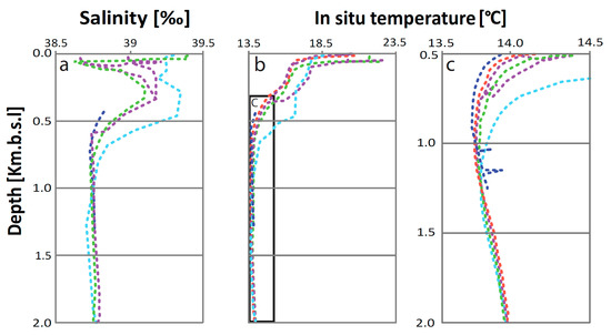
Figure 2.
Seawater salinity (a) and temperature (b) profiles, measured in various locations in the EMS by CTD casts in the course of four different cruises (6901084-06/2012-red, 6901043-09/2012-green, 6900850-10/2011-purple, 6900794-01/2009-azure; from [90]) and during EV Nautilus 11/2011 ROV survey ([69]; blue). (c) A zoom of the in situ temperature profiles (b) in the water depth range of 0.5 to 2 km.
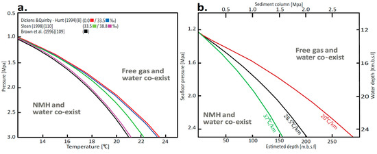
Figure 3.
A comparison of modeled methane hydrate stability curves. (a) The equilibrium curves predicted by the different modeling schemes considered in this work [8,109,110] under different constant salinity conditions (as color-coded at the top). (b) The effect of different temperature gradients (color-coded as noted) on the depth below the seafloor of the base gas hydrate stability zone (GHSZ) predicted by CSMhyd [89] with a constant salinity of 38.8‰, as a function of the seafloor water depth.
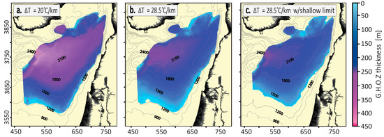
Figure 4.
The model predicted the extent and thickness (color coded on the right) of the potential gas hydrates occurrence zone (GHOZ) below the Levant Basin seafloor (plotted with UTM coordinates in km). (a) The GHOZ estimated by the sub-seafloor part of the GHSZ under a geothermal gradient of 20 °C/km. (b) The GHOZ estimated by the sub-seafloor part of the GHSZ under a geothermal gradient of 28.5 °C/km. (c) The GHOZ, estimated from the GHSZ under a geothermal gradient of 28.5 °C/km and top bound 25 m below the seafloor, as inferred from the presence of the shallow high amplitude seismic reflectivity (HASR) (see Section 4.5 text). This map constitutes our conservative estimate for the potential GHOZ in the Levant Basin.
2.2. Seismic Data and Analysis Methodology
The seismic component of this work is based on the analysis of five commercially acquired and processed 3D seismic blocks, and one 2D seismic profile (Table 1). The 3D blocks cover together (with some minor overlaps) a significant portion of the southern to central parts of the Levant Basin (Figure 1) between water depths of 900 to 1900 m, while the 2D profile connects the deepest 3D coverage with the eastern margin of the basin. The different data products that were available for our analysis vary in their exact processing and amplitude levels (Table 1), but were all processed through standard commercial workflows yielding zero phase amplitude preserved data. Thus, although not rigorously accurate the relative amplitudes are meaningful, at least in the region of interest within the first hundreds of meters beneath the seafloor. This assumption was asserted by us through manual visualization of the data, as well as through the calculation of amplitude histograms for each dataset.

Table 1.
The seismic datasets used.
All data were loaded to a Paradigm multi-survey project desktop for analysis. The time-migrated data two-way-times (TWT) were scaled to depth using constant seismic velocities of 1520 and 2000 m/s for the water and post-Messinian sedimentary column respectively. These velocity approximations were established through a comparison of overlapping regions of available depth migrated volumes and time migrated volumes and 2D profiles transecting them. We estimate the resulting depth errors to be ±5 and ±10 m for the seafloor and top Messinian (M) horizon respectively. These errors are approximately identical to the nominal resolution of the seismic reflections from the same depths. Paradigm’s propagator module was utilized for supervised automatic picking of the seafloor horizon, yielding a detailed bathymetric map at the resolution of each of the 3D seismic blocks. 3D shaded relief views of these bathymetric maps (e.g., Figure 5) were used to manually map the distribution of seafloor pockmarks and additional seafloor features.
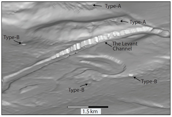
Figure 5.
A 3D shaded relief view of the high-resolution bathymetry, extracted from the Southern Israel 3D seismic data, across the southern part of the Levant channel within the Southern Israel block (see Figure 1 for position), viewed from the northwest. The pockmarks observed are classified into two types based on their sizes and morphologies. Type-A are oddly shaped large (hundreds of meters) scale pockmarks, while Type-B are generally rounded pockmarks ranging in diameter between 50 to 150 m.
This study examines the correlation of high amplitude reflectivity identified in the seismic datasets across the basin (the HASR; Figure 6, Figure 7 and Figure 8) with the GHSZ modeling results. The distribution of the HASR within the post-Messinian sedimentary stack was evaluated by two independent methods. Initially the HASR was manually picked on every 100th inline section and then on every 100th crossline section throughout each of the 3D blocks. The seafloor and HASR picks were then jointly outputted and their distributions were plotted using Matlab (Figure S1 in Supplementary Materials). To verify the correlation revealed, we repeated the process through a more rigorous automatic picking procedure. A sub-volume was extracted from each of the seismic blocks stretching 5 to 300 mbsf, eliminating the seafloor reflection above and the Messinian reflection below. The amplitude histograms of the sub-volumes extracted from each block were calculated, and a scaling factor to normalize the histograms of the different blocks was determined. Each of the sub-volumes was then loaded to Paradigm Voxel utility, where the HASR was picked by threshold detection. Following testing we established the threshold at the top 0.65% of the normalized histogram negative amplitudes tail. The picks were then converted to multi-valued horizons and outputted to Matlab distribution plots (Figure 9) and Paradigm spatial plots (Figure 10).
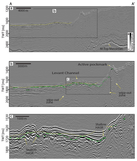
Figure 6.
Seismic time migrated section A-A’ (Figure 1) of the Southern Israel 3D data. The yellow dashed line represents the base GHSZ modeled with a thermal gradient of 28.5 °C/km on the regional bathymetric digital elevation model (DEM), while green dots represent the automatic HASR picks. (a) The full extent of the section down to the top of the Messinian evaporites (M). (b) A zoom on the rectangle in (a), showing the positions of ROV-surveyed active methane seepage site at the top pockmark of Palmahim disturbance and in the Levant Channel [69,70,71,84] and the Shallow HASR. (c) A zoom on the Levant channel area (the rectangle in (b)) showing the segmented appearance and mostly negative polarity of the HASR.
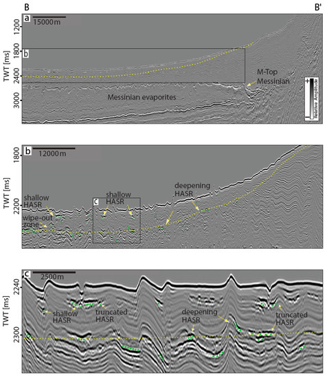
Figure 7.
Seismic time migrated section B-B’ (Figure 1) of the TGS IS-2069 2D profile. The yellow dashed line represents the base GHSZ modeled with a thermal gradient of 28.5 °C/km, while green dots represent the automatic HASR picks. (a) The full extent of the section down through the Messinian evaporites. (b) A zoom between 1780 to 2500 ms TWT in (a) showing the Shallow and Deepening HASR within the post-Messinian section. (c) A zoom on the rectangle in (b) depicting the truncated appearance and changing polarity of both the Shallow and Deepening HASR.
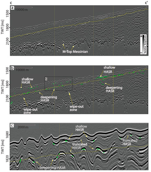
Figure 8.
Seismic depth migrated section C-C’ (Figure 1) of the Pelagic 3D data. The yellow dashed line represents the base GHSZ modeled with a thermal gradient of 28.5 °C/km, while green dots represent the automatic HASR picks. (a) The full extent of the section down to the top of the Messinian evaporites (M). (b) The same as in (a) with an overlay of the automatic HASR picks (green dots). (c) A zoom on the rectangle in (b) depicting the truncated appearance and mostly negative polarity of both the Shallow and Deepening HASR.
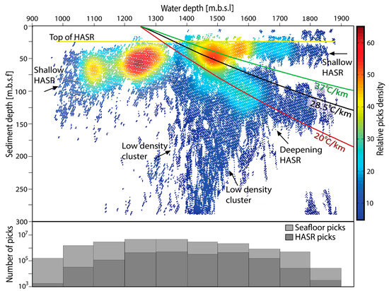
Figure 9.
The distribution of automatic HASR picks with respect to the seafloor water depth and the sediments depth below the seafloor. The color scale (right) represents the relative density of picks, i.e., the number of picks found in every 1 × 1 m bins. Overlain curves are the base GHSZ models for geothermal gradients of 20 °C/km (red), 28.5 °C/km (black), and 37 °C/km (green). The Shallow and Deepening HASR clusters are evident as distinct trends of high picks distributions. The histogram at the bottom shows the total number of positions (traces) in the seismic data (light gray) and the number of automatic HASR picks in 100 m intervals of the seafloor depth. This histogram demonstrates the validity of our picks distribution.
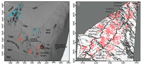
Figure 10.
(a) A shaded relief map of the southeastern part of the Levant Basin bathymetric DEM [62,108] overlaid with the spatial distribution of the HASR automatic picks and pockmark clusters within the different 3D seismic blocks analyzed. Black dots mark the Shallow HASR, while blue dots mark the Deepening HASR. Red ellipses mark the location of pockmark clusters. This figure demonstrates the wide distribution of Shallow HASR picks across the Levant Basin; the concentration of pockmark clusters between water depths of 900 to 1300 m across the deep fan of the Nile; and the distribution of the Deepening HASR at water depths >1300 m. (b) A zoom on the Pelagic 3D seismic block with the pronounced shading of the bathymetry (enhanced gray scale) overlaid with the automatic picks of the Shallow HASR (red). This figure demonstrates the relation between the Shallow HASR and seafloor channels of the Nile fan.
3. Results
3.1. Establishing the Local Environmental Conditions in the Deep Levant Basin
3.1.1. Bottom Water Temperature and Salinity
Bottom water temperatures and salinities of the Levant Basin were acquired from two independent data sets. The first consists of four vessel-based conductivity and temperature depth (CTD) casts surveys, collected between the years 2009 to 2012 to water depths >1500 m, and extracted from the EU PERSEUS consortium on-line repository [90]. The second data set consists of underwater remotely operated vehicle (ROV) based CTD measurements collected in the course of E/V Nautilus 2011 survey offshore Israel [69].
These datasets combined constrain water body salinities in the range of 38.74 to 38.83‰ between water depths of 800 to 2000 m (Figure 2). We therefore used an average salinity of 38.80‰ for the Levant Basin GHSZ model. The temperatures measured at the sea surface show sub-annual variability in the range of 16 °C to 28 °C (Figure 2). However, at a water depth of 800 m, constituting the top of the EMS deep water mass [91], water temperatures converge to a constant value of ~13.69 °C. The water temperature then increases at a rate of 0.015 to 0.02 °C per 100 m of water depth to in situ water temperatures of ~13.94 °C at a water depth of 2000 m. We therefore used a mean water temperature value of 13.80 °C for the deep water mass. This is the actual permanent temperature at the water depth interval of 900 to 1400 m. The values constrained here are consistent with other published values for the Levant region (e.g., [27,92,93]).
3.1.2. Sediment Salinity and Geothermal Gradient
As no data is currently published on pore water salinities in the Levant Basin seafloor, we used the same bottom water value of 38.8‰ also for the sub-seafloor salinity. This is probably a reasonable approximation considering a relatively high seawater content within the bottom sediments. Moreover, sensitivity tests (discussed below) demonstrate that the possible effects of salinity mis-estimations on our modeling results are minor.
The sediment temperature was calculated based on a constant seafloor temperature of 13.8 °C and a linear increase with depth amounting to the geothermal gradient. Published estimations of the geothermal gradient in the Levant Basin range between 20 to 37 °C/km, constituting the lower and upper bound estimates respectively. [94] used seafloor measurements to estimate geothermal gradients of ~37 °C/km at two stations within the Levant Basin. In contrast, [95] estimated based on the bottom-hole temperatures from several onshore wells as average geothermal gradient for northern and central Israel in the range of 22 to 25 °C/km. [96] estimated a vertical geothermal gradient in the range of 20 to 26 °C/km for the northern inland and offshore areas of the Nile fan. Their study is based on temperature data from 48 wells located adjacent to our study area. [97] estimated an average vertical geothermal gradient in the range of 20 to 30 °C/km based on temperature logs from wells in southern Israel. Most recently [86] suggested the average geothermal gradient of 28.5 °C/km, measured in the Yam-1 and Yam-2 wells in the southeastern margin of the basin (Figure 1), as an estimate for the Levant Basin geothermal gradient. However, [98] modeled the thermal history of the Levant Basin based on an interpreted chronostratigraphic framework of the basin and the measurements in four wells along its flanks (including apparently the Yam wells). In particular, this framework includes the presence of the ~2 km thick Messinian salt unit within the Basin and its absence in the flaks. Their modeling predicts geothermal gradients in the ranges between 20 and 28 °C/km and 13 and 20 °C/km in the Basin flanks and center, respectively. However, in the lack of published measurements from wells within the Levant Basin, the validity of these results to our GHSZ modeling is uncertain. It is notable that, in contrast to the significant impact of salt diapirs on NGH distribution in salt basins, such as the Gulf of Mexico (e.g., [99,100,101]), the relatively minor deformation of the Messinian salt in the Levant Basin is expected to inflict only limited variability on the GHSZ. Considering the high sensitivity of the GHSZ model to the geothermal gradient, and the uncertainty of its value, we created three versions of the GHSZ model using geothermal gradients of 20, 28.5, and 37 °C/km.
3.1.3. Pressure
Hydrates stability within the sediments depends on the interstitial pore pressure [1], generally bound between the hydrostatic and lithostatic pressure profiles [102,103]. At relatively shallow sediment depths of the GHSZ (normally <500 m [104]) in normally compacting basins sediments, porosity and permeability are generally high and the pore pressure is approximately hydrostatic or slightly above (e.g., [102,105]). We therefore assume a hydrostatic pore pressure profile in our GHSZ modeling. This assumption is supported by the pore pressure profile measured in Hanna-1 well, located at a water depth of 972 m in the eastern boundary of the study area (Figure 1), showing only a slight deviation from hydrostatic pressure within <500 m below the seafloor [106].
The hydrostatic pressure in the Levant Basin was calculated as a function of the depth below the surface using the equations of [107] in the range of 0.1–35.4 MPa. These equations estimate the pressure within maximal error bounds of 2 kPa, which are equivalent to depth errors <0.2 m. This is a negligible value in comparison with the water and sediment column depth-range of the GHSZ (>1000 m). These calculations were evaluated for each of the bathymetric grid cells as described below.
3.1.4. Bathymetry
To model the seafloor bathymetry of the Levant Basin we used a 250 m digital elevation model based on the bathymetric map of [62]. Across the exclusive economic zone of Israel, the bathymetry was updated based on a 250 m resolution bathymetric digital elevation model (DEM) released by the State of Israel, Ministry of Energy [108].
3.2. Electing a GHSZ Modeling Approach for the Levant Basin
To evaluate the adequate thermodynamic conditions for NGH formation, three different models of the GHSZ were tested [8,109,110]. These models use a phase diagram of solid methane hydrate versus liquid water and free gas phases (Figure 3). The models presented by [8,109] are empirical models, using a narrow range of temperature–salinity (T–S) conditions. In contrast, the model presented by [110] relies on statistical thermodynamics of the pressure–temperature (P–T) equilibrium conditions for methane hydrate stability and uses a wider range of T–S values.
Figure 3a presents the chemical equilibrium points predicted for the Levant Basin by these three models as a function of depth (i.e., pressure) and temperature, for a variety of constant salinity concentrations permitted by each of the methods and noted. The NGH stability zone is represented by the area below the curve predicted by each model; while above the curve water and free gas are predicted. The GHSZ is determined by cross-referencing the methane hydrate stability in the phase diagram with the seafloor bathymetric depth and the geothermal gradient. The results of the three different models diverge substantially from the Levant Basin conditions (Figure 3a). The results obtained by the models of [8,109] represent end-member solutions, while the results obtained by the [110] model fall between them.
Selection of the appropriate modeling scheme for this study is based on the following considerations: (1) The models by [8,109] are based on experimental data using pressure conditions that are below those predicted for the relevant depths in the Levant Basin; (2) the model suggested by [110] considers a salinity of 35.0‰, which is 3.8‰ lower than the Levantine average deep water salinity value; and (3) the use of the CSMHyd software implementation of [110] has become a standard for predicting GHSZ in related studies (e.g., [111,112]). Particularly, modeling of GHSZ at overlapping areas in the EMS using CSMHyd was recently performed by [29,65]. The Levant Basin GHSZ is therefore calculated in the present study based on the algorithms of [110], as implemented in the CSMHyd software [89].
In practice, CSMHyd was used to calculate the thermodynamic equilibrium pressure lookup table for temperatures values at increments of 0.02, 0.0285, and 0.037 °C, corresponding to the tested geothermal gradient, for pure methane hydrates and the EMS salinity. Then a Matlab code was used to search for the base GHSZ depth, by recursively calculating the pressure and temperature below the bathymetric depth. These were calculated based on the hydrostatic and geothermal gradients at a depth increment of 1 m, until the calculated equilibrium conditions were reached. The process was repeated for every point in the bathymetric DEM of the Levant with water depth >1250 m and the different geothermal gradients considered, yielding modeled maps of the base GHSZ (Figure 4). Finally, the modeled maps were loaded to the Paradigm Epos software and plotted over the seismic data to be compared with the trend of the observed seismic anomalies.
3.3. Model Sensitivities
Potential uncertainties in the modeling performed in this study might be introduced by the modeling methodology. Based on comparison with a large set of published experimental data of salt-inhibited hydrates stabilities, [110] evaluated CSMHyd modeled pressure (and therefore depth) predictions absolute errors at ~15%, which is unacceptable. However, these uncertainties cannot be attributed to CSMHyd alone, as they necessarily incorporate the experimental data measurement errors. These measurement errors are symmetrically distributed around CSMHyd’s predictions, and therefore may be averaged out [112]. Moreover, a divergence of the predicted and modeled values appears to be associated with larger temperatures and pressures than considered in this study (e.g., Figure 4 in [113]). In addition, the reliability of CSMHyd predictions was verified in a variety of studies, by their correlation with geophysical, well-log, and experimental results (e.g., [111,112,114,115,116,117,118]). Particularly, [119] employed a Monte-Carlo style simulation of their modeling uncertainties, which are similar to the uncertainties in this study (as discussed below), including explicitly CSMHyd 15% pressure prediction errors. They obtained a combined 1σ (one standard deviation) of most likely error estimate of ~±20 m at a water depth of 1240 m (Figure S2 in [119]) and decreasing values of the most likely error at increasing depths. Such uncertainties are acceptable in the context of the first-order evaluation performed in this study.
Additional errors in our modeling might be introduced by the average estimates and assumed values of the environmental parameters. Biased estimates of the bottom water temperature and salinity will affect the estimated water depth to the top of the GHSZ. This is also the seafloor depth at which the GHSZ pinches out laterally, and therefore defines the spatial extent of the GHSZ. Thus, with the ~1° slope gradient of the seafloor in the Levant, any bias on the top of the GHSZ will bias by a factor of c. ×50 the estimated potential lateral extent of hydrates across the basin seafloor. Similarly, biases in the interstitial salinity and geothermal gradient would bias the estimated depth below the seafloor of the GHSZ base. To evaluate the sensitivity of the model to our estimated salinity and temperature values we varied each of these parameters while keeping the other parameters fixed.
3.3.1. Water Temperature Effects
Temperature is the main factor affecting methane hydrate formation (e.g., [120,121]). The effects of water temperature uncertainties on the GHSZ model was evaluated by varying the modeled temperatures in steps of 0.1 °C within the range of 10–15 °C, keeping a constant salinity of 38.8‰. The results show a deepening of the GHSZ top by 4.2 m for every increase of 0.1 °C. The in situ temperature range of the Levant Basin bottom waters, as measured in the CTD surveys and the Nautilus expedition, is 13.69 to 13.94 °C (Figure 2). Thus, the expected temperature variation from the average temperature value is up to 0.13 °C, corresponding to a maximum shift of 5.9 m in the depth of the GHSZ base and a decrease of the estimated potential lateral extent of hydrates by ~600 m. This deviation represents error bounds of 0.05% in the modeled water depth on the top of the GHSZ. These error estimates are negligible in the context of this work.
3.3.2. Salinity Effects
An increase in salt content acts as an inhibitor to the formation of methane hydrate [110], and therefore would increase the water depth on the top of the GHSZ and decrease the depth of the GHSZ base beneath the seafloor. The sensitivity of the model results in an error in the estimated water salinity, which was examined by varying the salinity in steps of 0.25‰ in the range of 36.5 to 39.5‰, and by modeling the GHSZ with a constant water temperature. The results show a weak sensitivity of the variance in the GHSZ top boundary to the change in salinity. The slope of the salinity versus depth curve predicts a variance of 1.66 m in the depth of the GHSZ top for every shift of 0.25‰ in salinity. Consequently, a maximum error of 0.4 m, representing a deviation of 0.3‰, is introduced to the model by averaging the in situ salt concentrations of the Levant Basin bottom water values in the range of 38.74 to 38.83‰ (Figure 2).
3.3.3. Geothermal Effects
In order to determine the model sensitivity to different geothermal gradients, we modeled the two endmember models with the 20 and 37 °C/km geothermal gradients, and the in-between model with the 28.5 °C/km geothermal gradient (Figure 3). Changing the geothermal gradient does not change the top of the GHSZ, which is within the water body and therefore independent of the geothermal gradient (e.g., [8]). However, the different geothermal gradients result in significant deviations of the base of the GHSZ. The geothermal effect is best reflected in the differences between the different modeled base of GHSZ curves in Figure 3b. The depth of the base GHSZ at a water depth of 1800 m ranges between ~150 m under the low geothermal gradient of 20 °C/km, ~110 m calculated under the medium geothermal gradient of 28.5 °C/km, and ~85 m calculated under the high geothermal gradient of 37 °C/km. This paper discusses therefore the implications of these three alternative geothermal gradient models.
3.4. The Modelled Distribution of the GHSZ in the Levant Basin
Integrating the Levant pressure–temperature–salinity parameters into the model of [110] reveals that the GHSZ stretches widely across the Levant Basin (Figure 4). An initial estimate for the potential gas hydrates occurrence zone (GHOZ) (e.g., [1]) is provided by the sub-seafloor thickness of the GHSZ. Figure 4a,b presents the potential GHOZ thickness calculated and mapped for two of the alternative geothermal gradient estimates discussed above, namely the 20 °C/km and 28.5 °C/km geothermal gradients, respectively. A comparison between these maps (Figure 4a,b) provides an insight to the possible uncertainty in the implications of our modeling. The top of the GHSZ is located in both cases at the water depths of 1250 m, which limits the extent of the GHSZ to the northwestern two thirds of the basin. The thickest potential GHOZ is observed within the Cyprian trench at water depths of up to 2700 m, and it gradually thins to the south and east. The constrained depth to the base of the GHSZ (and therefore the potential thickness below the seafloor of the potential GHOZ) in the Levant is highly dependent on the geothermal gradient assumed, as discussed above. The base of the potential GHOZ at the deepest part of the study area is 431 and 260 m below the seafloor for the two alternative geothermal gradient estimates of 20 °C/km and 28.5 °C/km, respectively (Figure 4). The median modeled thicknesses of the potential GHOZ within the Levant Basin are ~200 and ~150 m respectively, when applying the same geothermal gradients.
3.5. Seismic Evidence for the Presence of Gas and Hydrates in the Southwestern Levant Basin
Considering the wide distribution of the GHSZ within the Levant Basin, the presence of hydrates is mainly conditioned on the presence of methane within the sediments. As pervasive sampling of the Levant sub-seafloor sediments is lacking, we seek preliminary evidence for the presence of methane through the analysis of an extensive set of available 3D seismic data.
3.5.1. Pockmarks in the Southeastern Levant Basin
Precise picking of the seafloor reflection in the 3D seismic volumes allows a detailed search for bathymetric features commonly associated with the presence of gas. Analysis of the high-resolution bathymetry available across the 3D seismic blocks identified the Palmahim disturbance fold crests group consisting of seven oddly shaped pockmark clusters measuring hundreds of meters across (Type-A; Figure 5); and a total of 160 smaller pockmark structures ranging in diameter between 50 to 150 m (Type-B; Figure 5). While a few of the identified pockmarks may represent errors in the seafloor maps, the majority of the features are robustly mapped and identified. The pockmarks are identified only in the Southern Israel, Gal-C, and Oz seismic surveys covering the base of the continental slope of southern Israel and the adjacent eastern part of the deep sea fan of the Nile region (Figure 1 and Figure 10). The pockmarks were detected in water depths of 1000 to 1300 m, and 90% of them are concentrated in four large clusters. Three of the clusters, which include 70% of the identified pockmarks, are located around a water depth of 1200 m, closely corresponding to the top of the GHSZ at 1250 m. Two of the clusters are located in the Nile deep sea fan region, and the other two (including the Palmahim Disturbance group) are located at the base of the continental slope of southern Israel.
3.5.2. Characteristics of Seismic Reflectivity in the Southern Levant Basin
A variety of reflectivity patterns characterize the top (post-Messinian) sedimentary section below the seafloor of the southeastern part of the Levant Basin, as imaged by the pervasive seismic dataset investigated in this work. The continental margin of Israel, in the eastern part of the investigated area, is characterized by relatively continuous and generally moderate amplitude reflections interleaved with chaotic intervals (Figure 6 and Figure 7). The latter representing mass transport complexes (MTC). This westward thinning, regionally up to ~6° dipping sedimentary section, was described in detail by [122], was based primarily on the Southern Israel 3D seismic volume. The top sedimentary section of the Nile submarine fan, to the west of the Israeli margin, was described by [46,47] based on detailed investigations of the Gal-C 3D seismic volume. The seismic reflectivity in this area (Figure 6, Figure 7 and Figure 8) is characterized primarily of locally segmented and dipping sets of reflections, representing channel levee complexes, embedded between coherent packages of locally continuous sub-parallel reflections, representing layered hemi-pelagic sediments. Intervals of chaotic reflectivity correspond to MTCs. This entire sedimentary package gently thins northward, and is folded and truncated by numerous thin-skinned sin-depositional halokinetic faults and ~100 m high folds. The bottom ca. third of this sedimentary stack, above the prominent M reflection, is generally characterized by relatively continuous high-amplitude reflections. Above this unit and up to ~100 m below the seafloor the section is generally characterized by moderate to low amplitude reflections.
A discontinuous band of segmented and scattered anomalously high-amplitude reflectivity (the HASR) is consistently observed within the top of the sedimentary stack, down to >100 m beneath the seafloor, throughout the Nile deep sea fan domain of the southeastern Levant Basin (Figure 6, Figure 7 and Figure 8). Much of the HASR display clear reversed polarity with respect to the seafloor reflections (e.g., white primary phase in Figure 6c, Figure 7c and Figure 8c), which usually implies a reduction in the seismic impedance across the sub-surface reflector. However, in many cases the HASR polarity is normal (the same as the seafloor, e.g., Figure 8c), or indistinguishable and laterally changing (e.g., Figure 6c). These changes in the polarity of the HASR do not seem to consistently represent certain datasets, or distinct ranges of water or sediment depths. High-amplitude reversed polarity reflectivity, similar to the reverse polarity HASR, is commonly considered as a direct indication for the presence of free gas within the sediments, while hydrates are commonly expected to be associated with normal phase high amplitude seismic reflectivity (e.g., [24]). However, similar reflectivity characteristics may alternatively represent abrupt changes between lithologies, physical integrities (e.g., porosities), or the impact of thin layers tuning (e.g., [24]). The HASR appears as anomalous segments within more continuous moderate amplitude reflections, or as separate reflectivity phases (Figure 6, Figure 7 and Figure 8). Segments of the HASR extend ~0.1 to several kilometers horizontally, and predominantly one, but sometimes up to several, seismic reflectivity phases (i.e., tens of meters) vertically. Neighboring segments are frequently vertically offset by up to several tens of meters with respect to each other; and in many cases, segments extend parallel to each other. Zones of amplitude wipe-outs (seismic amplitude blanking) extend in places hundreds of meters below the HASR concentrations, presumably the effects of seismic scattering and pronounced attenuation at the HASR levels. In general, no HASR is observed below the seafloor of the Israeli continental margin, with the exception of the folds at the western end of the Palmahim disturbance and their vicinity (Figure 1 and Figure 6). The active methane seeps discovered within large-scale pockmarks at the crests of these folds [69,70,71] are underlain by pronounced high amplitude and reverse polarity reflections, just (<10 m) beneath the seafloor (Figure 6). These reflections and additional reflectivity segments observed beneath the slopes of these folds to the west of the pockmarks, appear to represent a prolongation of the Nile deep sea fan HASR. Below water depths of 1400 to 1500 m the HASR band becomes less distinct and appears to extend deeper (down to ~200 m) into the sedimentary section (Figure 7 and Figure 8). Below water depths of >1500 m the HASR appears to separate into two branches: the first remains relatively coherent and limited to <100 m below the seafloor, while the other is characterized by localized enhancement of reflections of the moderate and higher amplitude sequences discussed above. This deeper branch of the HASR is sometimes harder to distinguish from the deeper higher amplitude reflections. However, in places it is distinctly apparent, mainly where amplitudes increase along a reflection and then abruptly diminish to a moderate amplitude reflection (Figure 7 and Figure 8).
3.5.3. Vertical Distribution of the HASR
To assess the relation of the HASR with the possible presence of NGH in the southeastern Levant Basin we evaluate the spatial distribution of the HASR and compare it to the GHSZ modeling predictions. This evaluation was done first through manual picking and then repeated through automatic threshold detection of high amplitude negative phase reflections, representing the HASR, throughout our combined seismic dataset (as detailed above). Figure 9 displays the distribution of the automatically detected HASR in depth within the sediments (depth below the seafloor) as a function of the water depth, and compares it to the modeled depths below the seafloor of the base of GHSZ. This plot lumps together the different surveys representing a wide range of water depths and geological settings across the continental slope of Israel and the deep sea fan of the Nile. Figure 9 also compares the statistics of the HASR picks to the statistics of the entire dataset, inspecting for possible biases of the picking results by the depth distribution of the available data. This plot shows substantial data coverage through the water depths range of 900 to 1900 m, albeit with most of the data covering the water depth range between 900 to 1600 m (primarily around 1200 m). Thus, distribution of the picks is probably over emphasizing the distribution of the HASR around the water depth of 1200 m and under-emphasizing the distribution of the HASR at water depths >1500 m. Considering these reservations we suggest that the trends observed in Figure 9 are significant. We note that the HASR picking represents only the highest amplitudes of the HASR, above the threshold selected for the automatic picking. In practice, the HASR phenomenon is more widely spread in the seismic data, as observed by us during the manual inspection and picking.
The HASR picks plotted in Figure 9 combine three clusters in accordance with the general observations of the HASR described above. The first cluster trends sub-parallel to the seafloor throughout the water depths >1000 m, while essentially no HASR picks were detected at water depths <1000 m. Between water depths of ~1000 to 1350 m this cluster is distributed primarily between 25 to ~120 m below the seafloor. The HASR in this population trends slightly to shallower sediments depths (beneath the seafloor) with increasing water depth, which is expressed in three ways: (1) The top boundary of the picks starts at a sediments depth of 40 m at the water depth of 1000 m, and ascends to a sediments depth of 25 m at a water depth of 1350 m; (2) high density patches of HASR picks are centered around the sediments depth of 70 m at the water depth range of 1050 to 1150 m, and around a sediments depth of 55 m at the water depths of 1200 to 1300 m (Figure 9); (3) the bottom boundary of the HASR ascends from a sediments depth of 90 to 150 m as the water depths increase between 1000 to 1350 m respectively, although this trend is characterized by a high scatter (Figure 9). In the water depth range of 1350 to 1900 m the first cluster of picks continues trending at a generally constant depth below the seafloor (Figure 9). The top boundary of the picks is generally 25 m below the seafloor, except for the several limited patches of picks appearing at shallower depths (Figure 9). The bottom boundary of this part of the first cluster is between 50 and 60 m below the seafloor. This first cluster of picks is referred to as “Shallow HASR” hereafter.
A second cluster of picks branches down from the Shallow HASR around the water depth of 1400 m (between water depths of 1300 and 1500 m) and a sediments depth of ~60 m, and trends to higher sediments depths with increasing water depths (Figure 9). The upper boundary of this cluster deepens to a sediment depth of 100 m at a water depth of 1900 m. A general lack of picks clearly distinguishes this cluster at water depths >1500 m from the Shallow HASR above. The majority of HASR picks in this cluster are concentrated between water depths of 1350 to 1670 m, with a more sporadic distribution continuing along the same trend to deeper water. This reduction in the density of the picks is probably at least partly reflecting the significant reduction in the distribution of available data covering this water depth range. Overall this cluster trends from 60 to 125 m below the seafloor (Figure 9). The bottom boundary of this population is not distinct as that of the upper HASR and is determined mostly by the decline in picks density with depth (Figure 9). This second cluster of picks is referred to as ”Deepening HASR” hereafter. An additional low-density cluster of HASR picks appears at water depths of 1200–1650 m, extending to a sediment depth of 300 m. This low density cluster does not display a consistent orientation and is detached from the main populations described above. This third cluster of picks represents to a great extent the lower unit of the sedimentary stack described above (e.g., Figure 6a), which is characterized by generally relatively continuous high-amplitude reflections. Owing to the deepening of the seafloor, this unit crosses from 200 to 300 m sediments depth at a water depth of ~1300 m, to a depth <100 at water depths >1600 m. Note however, that the Deepening HASR is represented by a substantial increase in picks density, and its trend clearly cuts through the lower reflective sedimentary unit, represented by the third low density cluster of picks (Figure 9).
Overlaying the HASR distribution with the modeled base-GHSZ depth curves (Figure 9) reveals that the trend and projected intercept of the Deepening HASR cluster is generally matched by the curve modeled with the 20 °C/km geothermal gradients, while the curve modeled with the 28.5 °C/km geothermal gradient appears to bound the upper extent of the Deepening HASR. This is verified also by overlaying the depths, predicted by the 28.5 °C/km geothermal gradient curve and bathymetric DEM, on the seismic data (Figure 6, Figure 7 and Figure 8). The resulting depth curve generally matches the upward truncations of the imaged HASR segments. Thus, there is a viable match between the HASR trend and a reasonable estimate of the base of GHSZ in the Levant Basin.
3.5.4. Spatial Distribution of the HASR
Map plots (Figure 10) reveal that the spatial distribution of HASR picks is uneven. The Shallow HASR is found in the deep sea fan of the Nile region, and is absent from the continental slope of Israel except for the tow region of the Palmahim disturbance. The Shallow HASR picks are mostly concentrated in patch sets reminiscent of foliage. Overlaying the distribution of the Shallow HASR with the bathymetry (Figure 10) reveals that the foliage-like patterns are aligned along the turbidite channels etched into the current seafloor and are branching downstream from them. Within each patch, the HASR picks depths below the seafloor are highly scattered, reflecting the laterally discontinuous nature of the HASR described above.
The distribution patterns of the Deepening HASR are reminiscent of the Shallow HASR patterns, but the spatial distributions across the basin of the two are considerably different. The Deepening HASR is mostly found in the western part of Sara-Mira and Pelagic 3D seismic surveys, as well as in the western part of the TGS 2D line (Figure 1 and Figure 6, Figure 7 and Figure 8). The deeper Deepening HASR are distributed at the top of the relatively high amplitude unit discussed above (Figure 6, Figure 7 and Figure 8), where they appear as discontinuous patches mostly limited to the elevated anticlinal parts of folding structures. A small portion of the picks is also sparsely distributed within the high amplitude unit (Figure 6, Figure 7 and Figure 8). Yet, these picks do not show any continuity and cannot be attributed to a specific reflecting horizon of this unit. Minor occurrences of the Deepening HASR are recognized also in the deeper parts of Gal-C, Sothern Israel, and Oz surveys, where the rare picks mainly appear along the surface of meandering channel paths around the paleo-channel canyons and in close proximity to faulted or folded structures (Figure 10).
4. Discussion
4.1. The GHSZ in the Levant Basin
The main purpose of this study is to review possible evidence and constrain the potential for the presence of NGH in the Levant Basin, southeastern Mediterranean, notwithstanding the current lack of direct evidence. For this purpose, we modeled the GHSZ in the Levant Basin based on the local thermodynamic conditions and salinity of the bottom water and interstitial pores in the sub-seafloor sediments. The bottom seawater conditions are relatively well constrained by data and therefore the definition of the top of the GHSZ to 1250 ± 5 m water depth is robust. This modeled top of the GHSZ is consistent with the shallowest water depth in which NGH occur in the Anaximander region, at a water depth of 1264 m at the summit of the Thessaloniki mud volcano [63,64]. [63] argued that this occurs at the top boundary of their modeled GHSZ, considering very similar local thermodynamic conditions to those used in this study. [65] observed the disappearance of the hydrates coating at a water depth of 1350 m, and estimated the top of the GHSZ in the western submarine fan of the Nile as 110 m deeper than our estimate for the Levant. This inconsistency may be explained by possible slightly elevated water temperature, and by the different gas composition in the cold seep sampled by [65].
The intersection of the modeled top of GHSZ with the bathymetry outlines the spatial extent of the potential GHOZ (Figure 4). The GHSZ stretches over more than half of the Levant Basin seafloor, constituting the vast majority of its central and northern parts. With the shortage of reliable data, approximations had to be made for the geothermal, pressure, and salinity profiles within the seafloor sediments. Yet, supported by indirect evidence and sensitivity analyses we argue that the modeled GHSZ presented here provide useful first-order approximated bounds of the possible distribution of NGH in the Levant Basin. The differences between the alternative maps of Figure 4a,b probably offer an over estimation of the uncertainty bounds in determining the depth below the seafloor to the base of the GHSZ. We suggest that the model calculated with a geothermal gradient of 28.5 °C/km (Figure 4) provides a conservative estimate of the depth to base of the GHSZ in the Levant Basin.
4.2. Methane and Hydrates in the Levant Seafloor Sediments
The actual in-place occurrence of NGH within the GHSZ is dependent on the availability and steady flow of methane gas within the sediment (e.g., [123]), and on the storage capacity of the sedimentary medium (e.g., [124]). The presence of an active gas system within the Levant Basin seafloor sediments is indicated by two main lines of evidence: direct evidence for seafloor gas seepage and geophysical indicators for the potential presence of gas.
4.2.1. Direct Evidence for Gas Seepage at the Seafloor
The multiple direct observations of active seafloor gas seeps within the perimeters of the Levant Basin [68,69,70,71,84] were all documented within a water depth range of 1000–1200 m, while the upper bound of the modeled GHSZ is at a water depth of 1250 m. Consequently, our model of the GHSZ in the Levant does not directly link the observed gas seeps and the possible upward percolation of methane from NGH within the GHSZ. Such a connection would require significant upslope lateral flow of methane. A possible indirect evidence for shallow gas emission is presented by the occurrence of pockmarks across the seafloor, as mapped based on the analyzed 3D seismic surveys (e.g., Figure 5 and Figure 10). These pockmarks appear to be limited to a water depth range of 1000–1300 m (Figure 10), correlating well with the spatial distribution of the edge of the modeled GHSZ and suggesting a possible tunneling of free methane gas along the base of the GHSZ toward its edge. Tunneling of methane to the edges of the GHSZ is attributed to the base of the GHSZ functioning as a seal that prevents gas escapes and tunneling the gas toward the GHOZ pinch out (e.g., [2,23,125]). Additionally, the pockmarks depth distribution might represent a record of the shift of the top of the GHSZ, and therefore the migration of the pinch out of the GHOZ to deeper water. The warming event at the end of the last glacial period, ~14.5 ka, was estimated to have raised the bottom water temperature in the Western Mediterranean by ~4 °C [126]. Assuming accordingly ~4°C cooler bottom waters in the Levant Basin (being ~10 °C) at ~14.5 ka, the modeled top of the GHSZ would occur at a water depth of ~890 m. This estimate is also consistent with the results of [29]. Phase delays between faster sea level changes [127] and slower warming of the Levant bottom water, such as suggested for the Arctic Ocean by [111], may have further facilitated the formation of NGH deposits and their subsequent destabilization. These processes may have resulted in enhanced gas release and seepage along the retreat path, and formed the observed pockmarks and authigenic carbonates. This, however, remains a hypothesis until the ages of seepage and carbonate precipitation are constrained.
4.2.2. The HASR–Evidence for Free Gas and Possibly Hydrates
The second line of evidence for the presence of gas in the seafloor sediments of the Levant Basin relies on the interpretation of the distinct HASR imaged off the deep-water shallow sediments of the studied area. We suggest that the HASR is associated with the presence of free gas, and possibly in at least some of the region with hydrate accumulations, within the upper sedimentary section. The correlation of high amplitude seismic reflectivity and underlying seismic amplitude blanking with subsurface gas bearing intervals is a commonly observed result of the strong response of seismic waves to the presence of even minor free gas content (e.g., [103,128]). High amplitude reflections may also be associated with hydrate accumulations within the GHSZ (e.g., [24,101,129]). Notably, high amplitude seismic reflections may alternatively represent other sub seafloor features in our study area, such as the prominent lithological and porosity contrast between shale layers and porous sand bodies lacking any presence of gas or hydrates. The reverse polarity of much of the HASR indicates low impedance intervals within the generally clay rich seafloor of the Levant basin, reinforcing the suggested presence of free gas (e.g., [117]). The normal or indistinguishable polarity observed in many of the cases may represent hydrate bearing intervals within the GHSZ, but seems puzzling outside and below the GHSZ. However, reflection polarities may be elusive due to thin layers tuning and structural complexities, particularly when the reflectors are segmented or discontinuous. Such polarity complexities are commonly observed where free gas and hydrates occur within discordant sedimentary intervals (e.g., [101,129]). In these cases, unraveling the polarity information requires focused analysis [130], which is outside the scope of this study. A central base for our interpretation is the unambiguous correlation of seafloor methane gas seepages, which were verified by seafloor surveying and sampled in the study area [68,69,70,71,84], with HASR just below the seafloor (e.g., Figure 5). Taking together the seismic characteristics with these direct verifications of methane gas seepage, we argue that at least part of the HASR represents the presence of free methane gas and possibly also the hydrates within the seafloor sediments. We note that the generation of reflectivity by the presence of free gas bubbles within the sediments requires methane saturation within the interstitial pore water (e.g., [131]). Thus, the observation of gas related HASR below the seafloor implies a significantly larger availability of dissolved methane for the formation of hydrates within the sediments, at least in parts of the Levant Basin.
4.2.3. The Shallow HASR–Evidence for Shallow Gas beneath the Levant Basin Seafloor
The vertical distribution of the observed Shallow HASR picks cluster is sub-parallel to the seafloor (Figure 9) and does not appear to depend strongly on the water depth or pressure. Neither does it appear to match the trend of any of the possible hydrate stability curves. Moreover, it clearly extends laterally significantly outside of the GHSZ, which is limited by the 1250 m water depth contour (Figure 10). We therefore suggest that at least outside the GHSZ the HASR represents primarily free methane gas accumulations in the shallow sub-seafloor sediments. Within the GHSZ region, bounded by the 1250 m water depth contour (Figure 10), the Shallow HASR may similarly represent hydrate concentrations. If the HASR represents hydrates then the upper cutoff of the HASR probably represents the top of the GHOZ, which is usually located tens of meters below the seafloor (e.g., [1,132,133]). Alternatively, the HASR may also represent the presence of free gas within the upper part of the GHSZ. Such occurrences of free gas within the GHSZ are indicated by seafloor bubbles emanations in cold seeps above hydrate bearing intervals [134]. The presence of free gas within the GHSZ have been suggested based on seismic reflectivity and velocity variations [135,136] as well as cone penetration test results [128]. In addition, high salinity, measured in boreholes drilled through hydrate bearing regions, is argued to be the product of free gas supply and hydrates formation within the GHSZ (e.g., [116]). Some mechanisms suggested for the maintenance of free gas within the GHSZ, which may apply for the Levant Basin, are: Transient focused flow through structural or lithological pathways (e.g., [116,135]); local increase of pore water salinities as a result of proximate NGH formation, allowing the stability of free gas within the GHSZ [114,116]; and low sediment permeability resulting in insufficient water supply for NGH formation to the zone containing free gas [128].
Whether the Shallow HASR represents free gas or NGH, both alternatives imply that the saturation of dissolved methane is exceeded in the interstitial pore water at their level [110]. The shallow cut-off of methane saturation in the marine environment, and therefore presumably also the top of the HASR distribution, is generally constrained by anaerobic oxidation of methane (AOM). The AOM is maintained below the sulfate methane transition zone (SMTZ) by balanced diffusion fluxes of methane from the saturated zone and sulfate from the seafloor (e.g., [137]). Reference [138] showed that the depth below the seafloor to the top of the free gas zone can be used to estimate the upward flux of dissolved methane, given in situ methane solubility (saturation). To examine the possibility of our interpretation of the HASR as related to methane free gas or hydrates, we followed the approach of [138] in estimating the upward methane flux based on the upper cutoff of the Shallow HASR distribution 25 m below the seafloor (see detailed derivation in the Supplementary Information). Based on [139,140] and the same thermodynamic conditions used in our GHSZ modeling we estimate that the methane solubility, related with the top of the Shallow HASR, is between 0.98 and 1.03 mmol, depending on the water depth. To estimate the balance of sulfate and methane fluxes at the SMTZ we assumed negligible methane production between the HASR and seafloor and linear concentration gradients. The resulting estimated methane fluxes are 9 to 20 mmol∙a−1∙m−2, corresponding to water depths rage of 1200 to 2000 m. These results are in agreement with the SMTZ distribution models and methane fluxes reported from NGH provinces across the globe, ranging between 20 and 250 mmol∙a−1∙m−2 [141,142,143,144,145,146,147]. Thus, these results support our interpretation of the seismic HASR as representing free gas or in-place NGH concentrations, both of which support the possible occurrence of NGH deposits within the modeled GHSZ.
The essentially exclusive occurrence of the Shallow HASR in the Nile deep sea fan (Figure 10) and their clear correlation with seafloor channels suggests a genetic relation between these phenomena. [46,47] demonstrated that the upper sedimentary section within the eastern deep sea fan of the Nile is composed of densely spaced relatively sand rich channel-levee complexes, encased within hemipelagic sediments. We suggest that these relatively sand rich bodies constitute localized reservoirs of free gas, and possibly also NGH, represented by the Shallow HASR. The foliage like pattern of the Shallow HASR, diverging from the current seafloor channels, suggest that the primary reservoirs for the Shallow HASR are paleo-lobes, associated with these channel systems, buried tens of meters below the seafloor. The scattered nature of the HASR within the observed patches probably represent the complexity of the channel-levee-lobe systems (e.g., as discussed by [148]) and their truncation by recent salt tectonics (as discussed by [46]). Similar associations of scattered free gas and hydrate accumulations with buried relatively sandy channel systems, and the observations of a diffuse BSR, have been reported from various large river deep sea fans. Examples are the Congo River [149], Godavari River [150,151], and the Pearl River [129].
4.3. The Deepening HASR–a Distributed BSR in the Levant Basin (?)
The locus and trend of the Deepening HASR picks cluster, mapped in the study area, appear to be approximately bounded by the modeled base-GHSZ with the 20 and 28.5 °C/km thermal gradients (Figure 9). The identification of the Deepening HASR on the seismic sections may appear somewhat arbitrary (Figure 7 and Figure 8), as the picked phases appear is some cases to be conformal with the generally relatively high amplitude reflections of the lower sedimentary unit in the study area. Indeed, picks scattered below the Deepening HASR and toward shallower water-depths do detect reflections within that layer. However, the Deepening HASR cluster represents an order of magnitude larger community of picks that are concentrated along this trend, demonstrating that it is subjectively anomalous with respect to the rest of the unit. A more careful inspection of the sections (Figure 7 and Figure 8) reveals the clear intensification of reflection amplitudes as they approach the Deepening HASR alignment (approximately demarcated in the figures by the overlaid base GHSZ modeled curves). Moreover, the pronounced amplitude reflections associated with the Deepening HASR commonly appear truncated in the upward direction, but in many cases can actually be traced farther with diminished amplitudes. Taking together the first-order match between the GHSZ model and the Deepening HASR, and their observed characters, we suggest that the Deepening HASR constitutes a segmented and distributed BSR, one of the primary indicators for the presence of NGH. Thus, the Deepening HASR is suggested to represent the presence of free gas trapped below the base of the GHSZ and possibly also hydrates deposited at the lower part of the GHOZ. The distributed nature of the Deepening HASR probably results from the distribution of free gas and hydrates in localized relatively sandy channel lobe systems (as discussed above for the Shallow HASR), the truncation of the lower unit sandy bodies by salt tectonics and possible variations of methane supply.
4.4. The Possible Sources of Methane
Two possible mechanisms may supply methane to the pervasive gas and possibly hydrate systems proposed here to exist in the Levant Basin. Methane may be supplied by in situ methanogenesis through bacterial decomposition of organic material (e.g., [152,153]). The methane generated by the bacteria within the GHSZ is incorporated in the NGH inside the GHSZ, while methane generated outside the GHSZ may form free gas bubbles. [154] modeled the case of methane diffusion to fine sandy layers from methanogenesis occurring in the surrounding fine grain intervals containing modest amounts (<0.5% of dry weight) of organic matter. This mechanism is concluded to be sufficient to supply the required methane for the formation of the hydrates observed in the Cascadia margin at IODP site U1325. Alternatively, methane transport through upward fluid flow from lower sedimentary levels may be important (e.g., [133,153]). In this case, the ascending gas is incorporated into the NGH structure or remains trapped below the layer of the NGH-containing sediments [1,155,156]. In either case, a possible source for hydrocarbons production is the abundant organic matter (up to 7%) buried in sapropel deposits throughout much of the post-Messinian sediments of the deep-water part of the Levant Basin [157,158,159]. The evident association of the HASR to the meandering channels and associated buried lobes may suggest an additional direct contribution of transported organic matter from the Nile River. Taken together the proximity of organic-rich sapropel units and coarse grain sizes (high porosity sediments) characterizing the infill of submarine channel-Levee-fan complexes [47,59] provide both possible sources and reservoirs for gas and hydrate formation and accumulation. The possible sources for organic matter discussed above, support the possible in situ formation of methane outside, below, and within the GHSZ. The deep giant gas reservoirs recently found in the Levant Basin [86,87], or related systems, are also possible gas sources for methane that may have been transported via migration paths such as faults and folds to the GHSZ. The existence of such migration paths within the southeastern Levant Basin was suggested by [80,82], but thorough connectivity has not been demonstrated as of yet.
4.5. Volume Assessment of Potential NGH Deposits in the Levant
Lacking conclusive indications, this study offers only suggestive evidences, raising the possibility for the presence of hydrates in the Levant Basin. Yet, our combined modeling and observations offer a first-order assessment of the NGH potential in the Levant Basin, with direct implications on potential energy resources, geohazard risk estimation, and models related to carbon cycles and its possible relation with present and future climate-change.
For this first-order assessment of potential NGH resources in the Levant Basin, we take the simplistic steady state assumption, while noting [123] discussion of the deficiencies of this assumption. In that case, NGH may form throughout the sedimentary column within the GHOZ, constrained by the isopach between the seafloor bathymetry and our modeled base GHSZ (Figure 4). Assuming that the intercept and trend of the Deepening HASR (Figure 9) represent a segmented and distributed BSR, the fit of the modeled base of the GHSZ curves with this trend constrains the relevant geothermal gradient between 20 to 28.5 °C/km within the post-Messinian sediments of the Levant Basin. Larger geothermal gradients, toward the 37 °C/km end member geothermal gradient, are not in agreement with the Deepening HASR being aligned with the base of the GHSZ. Thus, a maximum estimate of NGH potential is constrained by the map that was modeled using the lower geothermal gradient end member of 20 °C/km (Figure 4), while a more modest estimate is constrained by the map calculated with the higher 28.5 °C/km geothermal gradient (Figure 4). Consumption of methane at the SMTZ reduces its saturation, inhibiting the possible formation of NGH [141]. Thus, discarding the top of the sedimentary section, above the top cutoff of the Shallow HASR cluster, defines presumably a more reliable estimate of the sedimentary column available for hydrate accumulation i.e., the GHOZ. This estimate of the GHOZ is represented by the thickness map of Figure 4c with a total volume of ~3250 km3. The geothermal gradient of the Levant Basin (20 to 28.5 °C/km [86,94,95,96,97] is expected to be lower than in the adjacent Herodotus Basin and the Cypriot arc regions [160,161,162]. Thus, the GHOZ thickness map, which is based on the Levant Basin parameters, is expected to be less accurate toward these areas.
The discussion above suggests that hydrates in the Levant are primarily concentrated within relatively sandy channel-levee-lobe complexes. Based on our partial mapping of these silty to sandy bodies (Figure 10), we estimate them to occupy only ~3% of the sedimentary volume defined by Figure 4c. Considering a lower bound porosity of ~35% and hydrate saturation of ~50% for silt and sand rich host sediments [2,133] we obtain that NGH occupy on average ~0.5% of the sedimentary volume within the potential GHOZ (Figure 4c). Thus, considering a conservative NGH to gas yield factor of ~160 [4], the current study provides a first-order conservative estimation of ~100 Tcf (~2750 km3) for the potential volume (at standard temperature and pressure) of locked methane, and ~1.5 gigatonnes of carbon in NGH in the Levant Basin. These estimations constitute between ~0.1 to 3‰ of the estimated global NGH methane volumes and carbon content in marine sediments [2,4,5,163].
5. Conclusions
Seafloor gas seepages discovered in recent years in and around the Levant Basin, and sparse observations of hydrates in the broader EMS context are suggestive of the presence of NGH in the basin. Motivated by these findings this study combines thermodynamic modeling and analysis of a pervasive seismic dataset to examine the potential for such a presence.
- Thermodynamic modeling, using the CSMHyd software, robustly constrained by locally measured southeastern Mediterranean water temperature and salinity profiles reveals that the top of the GHSZ is at a water depth of 1250 ± 5 m. Intersecting this depth with the bathymetry reveals that more than half of the Levant Basin seafloor, namely its central to northern part, lies within the GHSZ.
- Modeling the base of the GHSZ is constrained by the lack of measured sub-seafloor thermodynamic parameters, and associated uncertainties. The primary modeling uncertainty is related with the availability and confidence of published sub-seafloor geothermal gradients. Yet, using simplistic approximations for the thermodynamic parameters yields a useful first-order approximation of the GHSZ within the Levant. The base of the GHSZ lies at a depth of 150 to 200 mbsf at a water depth of 1750 m, and may reach a depth of 430 mbsf at the northwestern edge of the studied area.
- Seafloor pockmark clusters observed in our seismic data are concentrated at a water depth of ~1200 m, just upslope from the modeled top bound of the GHSZ and mostly above the deep sea fan of the Nile. These pockmarks suggest the prominence of seafloor gas in the region, and may represent a partly ongoing gas seepage episode associated with the presumed downslope retreat of NGH since the last glacial time.
- Scattered high amplitude seismic reflectivity (HASR) is pervasively distributed beneath the seafloor across the deep sea fan of the Nile, correlating in several sites with observed active gas seepages. The HASR is therefore suggested to represent the wide spread presence of free gas, and possibly NGH, captured within buried distributed channel–levee related sandy/silty units.
- The distribution of the HASR depth beneath the seafloor vs. the water depth bifurcates into two main clusters. Most of the HASR across the study area cluster between 25 to 100 mbsf, and sub-parallel to the seafloor. This cluster is suggested to represent shallow free gas, and possibly hydrates, whose top is bounded by the SMTZ. An additional major HASR cluster trends to greater sub-seafloor depth with increasing water depth. The trend of this cluster broadly matches the modeled base of the GHSZ with a thermal gradient between 20 to 28.5 °C/km, and it is therefore suggested to represent a regionally discontinuous BSR beneath the Levant Basin. The discontinuity is attributed to the distributed nature of channel-lobes systems, into which the NGH and presumably underlying free gas are accumulated.
- Taken together, the modeling results and seismic analysis suggest the probable presence of NGH in the Levant Basin, within confined lithological bodies across the deep sea fan of the Nile. The presence of NGH is conservatively bounded between the base GHSZ modeled using the thermal gradient of 28.5 °C/km, and the SMTZ, which is estimated to occur ~25 m below the seafloor. Thus, the potential methane resource within the Levant Basin is estimated at ~100 Tcf, which would contain ~1.5 gigatonnes of carbon.
Supplementary Materials
The following are available online at https://www.mdpi.com/2076-3263/9/7/306/s1, Section S1: Methane flux and the sulfate methane transition zone (SMTZ); Section S2: Manual picking of the HASR; Figure S1: The distribution of manually picked HASR.
Author Contributions
Conceptualization, Y.M.; formal analysis, Z.T. and Y.M.; supervision, Y.M.; writing—original draft, Z.T., A.M., and Y.M.; writing—review and editing, Z.T., A.M., Z.B.-A., and Y.M.
Funding
This research was funded by the Moses Strauss Department of Marine Geosciences and Leon H. Charney School of Marine Sciences, University Haifa.
Acknowledgments
We thank the Oil Commissioner’s Office in the Ministry of Energy of the State of Israel, Modiin Energy, Genesis Energy (Israel) Ltd. for data sharing and permitting. We thank Paradigm for sponsoring the use of their software. We also thank O.M. Bialik, S. Pinkert, and three anonymous reviewers for their helpful comments, which significantly improved this paper.
Conflicts of Interest
The authors declare no conflict of interest. The funders had no role in the design of the study; in the collection, analyses, or interpretation of data; in the writing of the manuscript, or in the decision to publish the results.
References
- Sloan, E.D.; Koh, C. Clathrate Hydrates of Natural Gases, 3rd ed.; CRC Press: Boca Raton, FL, USA, 2008; p. 730. [Google Scholar]
- Boswell, R.; Waite, W.F.; Kvenvolden, K.; Koh, C.A.; Klauda, J.B.; Buffett, B.A.; Frye, M.; Maslin, M. What are gas hydrates. In Frozen Heat: A UNEP Global Outlook on Methane Gas Hydrates? Beaudoin, Y.C., Waite, W., Boswell, R., Dallimore, S.R., Eds.; United Nations Environment Programme; GRID-Arendal; Birkland Trykkeri A/S: Birkeland, Norway, 2014; Volume 1, pp. 11–30. [Google Scholar]
- Kvenvolden, K.A. Methane hydrate—A major reservoir of carbon in the shallow geosphere? Chem. Geol. 1988, 71, 41–51. [Google Scholar] [CrossRef]
- Milkov, A.V. Global estimates of hydrate-bound gas in marine sediments: How much is really out there? Earth Sci. Rev. 2004, 66, 183–197. [Google Scholar] [CrossRef]
- Klauda, J.B.; Sandler, S.I. Global distribution of methane hydrate in ocean sediment. Energy Fuels 2005, 19, 459–470. [Google Scholar] [CrossRef]
- Tréhu, A.M.; Ruppel, C.; Holland, M.; Dickens, G.R.; Torres, M.E.; Collett, T.S.; Schultheiss, P. Gas hydrates in marine sediments: Lessons from scientific ocean drilling. Oceanography 2006, 19, 124–142. [Google Scholar] [CrossRef]
- Piñero, E.; Marquardt, M.; Hensen, C.; Haeckel, M.; Wallmann, K. Estimation of the global inventory of methane hydrates in marine sediments using transfer functions. Biogeosciences 2013, 10, 959–975. [Google Scholar] [CrossRef]
- Dickens, G.R.; Quinby-Hunt, M.S. Methane hydrate stability in seawater. Geophys. Res. Lett. 1994, 21, 2115–2118. [Google Scholar] [CrossRef]
- Shipley, T.H.; Houston, M.H.; Buffler, R.T.; Shaub, F.J.; McMillen, K.J.; Ladd, J.W.; Worzel, J.L. Seismic evidence for widespread possible gas hydrate horizons on continental slopes and rises. AAPG Bull. 1979, 63, 2204–2213. [Google Scholar]
- Hyndman, R.D.; Spence, G.D. A seismic study of methane hydrate marine bottom simulating reflectors. J. Geophys. Res. 1992, 97, 6683–6698. [Google Scholar] [CrossRef]
- MacKay, M.E.; Jarrard, R.D.; Westbrook, G.K.; Hyndman, R.D. Origin of bottom-simulating reflectors: Geophysical evidence from the Cascadia accretionary prism. Geology 1994, 22, 459–462. [Google Scholar] [CrossRef]
- Berndt, C.; Bünz, S.; Clayton, T.; Mienert, J.; Saunders, M. Seismic character of bottom simulating reflectors: Examples from the mid-Norwegian margin. Mar. Pet. Geol. 2004, 21, 723–733. [Google Scholar] [CrossRef]
- Shedd, W.; Boswell, R.; Frye, M.; Godfriaux, P.; Kramer, K. Occurrence and nature of “bottom simulating reflectors” in the northern Gulf of Mexico. Mar. Pet. Geol. 2012, 34, 31–40. [Google Scholar] [CrossRef]
- Majumdar, U.; Cook, A.E.; Shedd, W.; Frye, M. The connection between natural gas hydrate and bottom-simulating reflectors. Geophys. Res. Lett. 2016, 43, 7044–7051. [Google Scholar] [CrossRef]
- Tsuji, Y.; Fujii, T.; Hayashi, M.; Kitamura, R.; Nakamizu, M.; Ohbi, K.; Saeki, T.; Yamamoto, K.; Namikawa, T.; Inamori, T.; et al. Methane-hydrate occurrence and distribution in the eastern Nankai Trough, Japan: Findings of the Tokai-oki to Kumano-nada methane-hydrate drilling program. In Natural Gas Hydrates—Energy Resource Potential and Associated Geologic Hazards; Collett, T., Johnson, A., Knapp, C., Boswell, R., Eds.; AAPG Memoir; American Association of Petroleum Geologists: Tulsa, OK, USA, 2009; Volume 89, pp. 228–246. [Google Scholar]
- Kvenvolden, K.A. Methane hydrate in the global organic carbon cycle. Terra Nova 2002, 14, 302–306. [Google Scholar] [CrossRef]
- Dickens, G.R. Rethinking the global carbon cycle with a large, dynamic and microbially mediated gas hydrate capacitor. Earth Planet. Sci. Lett. 2003, 213, 169–183. [Google Scholar] [CrossRef]
- Beaudoin, Y.C.; Waite, W.; Boswell, R.; Dallimore, S.R. (Eds.) Frozen Heat: A UNEP Global Outlook on Methane Gas Hydrates; United Nations Environment Programme, GRID-Arendal; Birkland Trykkeri A/S: Birkeland, Norway, 2014; Volume 2, p. 96. [Google Scholar]
- Dickens, G.R. Carbon cycle: The blast in the past. Nature 1999, 401, 752–755. [Google Scholar] [CrossRef]
- Kennett, J.P.; Cannariato, K.G.; Hendy, I.L.; Behl, R.J. Carbon isotopic evidence for methane hydrate instability during Quaternary interstadials. Science 2000, 288, 128–133. [Google Scholar] [CrossRef] [PubMed]
- Buffett, B.; Archer, D. Global inventory of methane clathrate: Sensitivity to changes in the deep ocean. Earth Planet. Sci. Lett. 2004, 227, 185–199. [Google Scholar] [CrossRef]
- Wallmann, K.; Dallimore, S.; Biastoch, A.; Westrook, G.; Shakova, N.; Severinghaus, J.; Dickens, G.; Mienert, J. Assessment of the sensitivity and response of Methane hydrate to global climatic change. In Frozen Heat: A UNEP Global Outlook on Methane Gas Hydrates; Beaudoin, Y.C., Waite, W., Boswell, R., Dallimore, S.R., Eds.; United Nations Environment Programme, GRID-Arendal; Birkland Trykkeri A/S: Birkeland, Norway, 2014; Volume 1, pp. 50–75. [Google Scholar]
- Sultan, N.; Cochonat, P.; Foucher, J.P.; Mienert, J. Effect of gas hydrates melting on seafloor slope instability. Mar. Geol. 2004, 213, 379–401. [Google Scholar] [CrossRef]
- McConnell, D.R.; Zhang, Z.; Boswell, R. Review of progress in evaluating gas hydrate drilling hazards. Mar. Pet. Geol. 2012, 34, 209–223. [Google Scholar] [CrossRef]
- Hecht, A. Abrupt changes in the characteristics of Atlantic and Levantine intermediate waters in the Southeastern Levantine Basin. Oceanol. Acta 1992, 15, 25–42. [Google Scholar]
- Lejeusne, C.; Chevaldonné, P.; Pergent-Martini, C.; Boudouresque, C.F.; Pérez, T. Climate change effects on a miniature ocean: The highly diverse, highly impacted Mediterranean Sea. Trends Ecol. Evol. 2010, 25, 250–260. [Google Scholar] [CrossRef] [PubMed]
- Sisma-ventura, G.; Yam, R.; Kress, N.; Shemesh, A. Water column distribution of stable isotopes and carbonate properties in the South-eastern Levantine basin (Eastern Mediterranean): Vertical and temporal change. J. Mar. Syst. 2016, 158, 13–25. [Google Scholar] [CrossRef]
- Miles, P.R. Potential distribution of methane hydrate beneath the European continental margins. Geophys. Res. Lett. 1995, 22, 3179–3182. [Google Scholar] [CrossRef]
- Praeg, D.; Geletti, R.; Wardell, N.; Unnithan, V.; Mascle, J.; Migeon, S.; Camerlenghi, A. The Mediterranean Sea: A natural laboratory to study gas hydrate dynamics. In Proceedings of the 7th International Conference on Gas Hydrates (ICGH 2011), Edinburgh, UK, 17–21 July 2011; pp. 17–21. [Google Scholar]
- Klauda, J.B.; Sandler, S.I. Phase behavior of clathrate hydrates: A model for single and multiple gas component hydrates. Chem. Eng. Sci. 2003, 58, 27–42. [Google Scholar] [CrossRef]
- Merey, S.; Longinos, N. Does the Mediterranean Sea have potential for producing gas hydrates? J. Nat. Gas Sci. Eng. 2018, 55, 113–134. [Google Scholar] [CrossRef]
- Fylaktos, N.; Papanicolas, C.N. New technologies for Eastern Mediterranean offshore gas exploration. In European Parliamentary Research Service; Scientific Foresight Unit (STOA): Brussels, Belgium, 2019; PE 634.419; p. 68. [Google Scholar]
- Minshull, A.M.; Marín-Moreno, H.; Betlem, P.; Bialas, J.; Buenz, S.; Burwicz, E.; Cameselle, A.L.; Cifci, G.; Giustiniani, M.; Hillman, J.I.T.; et al. Hydrate occurrence in Europe: A review of available evidence. Mar. Pet. Geol. in review.
- Garfunkel, Z. Constrains on the origin and history of the Eastern Mediterranean basin. Tectonophysics 1998, 298, 5–35. [Google Scholar] [CrossRef]
- Robertson, A.H.F. Mesozoic-Tertiary tectonic evolution of the easternmost Mediterranean area: Integration of marine and land evidence. In Proceedings of the Ocean Drilling Program, Scientific Results; Robertson, A.H.F., Emeis, K.C., Richter, C., Camerlenghi, A., Eds.; ODP: College Station, TX, USA, 1998; Volume 160, Chapter 54; pp. 723–782. [Google Scholar]
- Aksu, A.E.; Hall, J.; Yaltırak, C. Miocene–recent evolution of Anaximander Mountains and Finike Basin at the junction of Hellenic and Cyprus arcs, eastern Mediterranean. Mar. Geol. 2009, 258, 24–47. [Google Scholar] [CrossRef]
- Briand, F. (Ed.) The Messinian Salinity Crisis from mega-deposits to microbiology—A consensus report. In N° 33 in CIESM Workshop Monographs; CIESM: Monaco, 2008; p. 168. [Google Scholar]
- Meilijson, A.; Hilgen, F.; Sepúlveda, J.; Steinberg, J.; Fairbank, V.; Flecker, R.; Waldmann, N.D.; Spaulding, S.A.; Bialik, O.M.; Boudinot, F.G.; et al. Chronology with a pinch of salt: Integrated stratigraphy of Messinian evaporites in the deep Eastern Mediterranean reveals long-lasting halite deposition during Atlantic connectivity. Earth Sci. Rev. 2019, 194, 374–398. [Google Scholar] [CrossRef]
- Madof, A.S.; Bertoni, C.; Lofi, J. Discovery of vast fluvial deposits provides evidence for drawdown during the late Miocene Messinian salinity crisis. Geology 2019, 47, 171–174. [Google Scholar] [CrossRef]
- Gardosh, M.; Druckman, Y.; Buchbinder, B.; Rybakov, M. The Levant Basin Offshore Israel: Stratigraphy, Structure, Tectonic Evolution and Implications for Hydrocarbon Exploration; Geophysical Institute of Israel Report 429/218/06; Geophysical Institute of Israel: Lod, Israel, 2006; p. 118. [Google Scholar]
- Steinberg, J.; Gvirtzman, Z.; Folkman, Y.; Garfunkel, Z. Origin and nature of the rapid late Tertiary filling of the Levant Basin. Geology 2011, 39, 355–358. [Google Scholar] [CrossRef]
- Ryan, W.B. Messinian badlands on the southeastern margin of the Mediterranean Sea. Mar. Geol. 1978, 27, 349–363. [Google Scholar] [CrossRef]
- Gvirtzman, Z.; Reshef, M.; Buch-Leviatan, O.; Groves-Gidney, G.; Karcz, Z.; Makovsky, Y.; Ben-Avraham, Z. Bathymetry of the Levant basin: Interaction of salt-tectonics and surficial mass movements. Mar. Geol. 2015, 360, 25–39. [Google Scholar] [CrossRef]
- Macgregor, D.S. The development of the Nile drainage system: Integration of onshore and offshore evidence. Pet. Geosci. 2012, 18, 417–431. [Google Scholar] [CrossRef]
- Sestini, G. Nile Delta: A review of depositional environments and geological history. In Deltas; Sites and Traps for Fossil Fuels; Whateley, M.K.G., Pickering, K.T., Eds.; Geological Society of London: London, UK, 1989; pp. 99–127. [Google Scholar]
- Folkman, Y.; Mart, Y. Newly recognized eastern extension of the Nile deep-sea fan. Geology 2008, 36, 939–942. [Google Scholar] [CrossRef]
- Clark, I.R.; Cartwright, J.A. Interactions between submarine channel systems and deformation in deepwater fold belts: Examples from the Levant Basin, Eastern Mediterranean Sea. Mar. Pet. Geol. 2009, 26, 1465–1482. [Google Scholar] [CrossRef]
- Tibor, G.; Ben-Avraham, Z.; Steckler, M.; Fligelman, H. Late Tertiary subsidence history of the Southern Levant Margin, Eastern Mediterranean Sea, and its implications to the understanding of the Messinian event. J. Geophys. Res. 1992, 97, 17593–17614. [Google Scholar] [CrossRef]
- Buchbinder, B.; Zilberman, E. Sequence stratigraphy of Miocene-Pliocene carbonate-siliciclastic shelf deposits in the eastern Mediterranean margin (Israel): Effects of eustasy and tectonics. Sediment. Geol. 1997, 112, 7–32. [Google Scholar] [CrossRef]
- Schattner, U.; Lazar, M. Hierarchy of source-to-sink systems—Example from the Nile distribution across the eastern Mediterranean. Sediment. Geol. 2016, 343, 119–131. [Google Scholar] [CrossRef]
- Almogi-Labin, A.; Bar-Matthews, M.; Shriki, D.; Kolosovsky, E.; Paterne, M.; Schilman, B.; Matthews, A. Climatic variability during the last 90ka of the southern and northern Levantine Basin as evident from marine records and speleothems. Quat. Sci. Rev. 2009, 28, 2882–2896. [Google Scholar] [CrossRef]
- Castañeda, I.S.; Schefuß, E.; Pätzold, J.; Damsté, J.S.S.; Weldeab, S.; Schouten, S. Millennial-scale sea surface temperature changes in the eastern Mediterranean (Nile River Delta region) over the last 27,000 years. Paleoceanography 2010, 25, PA1208. [Google Scholar] [CrossRef]
- Ehrmann, W.; Schmiedl, G.; Seidel, M.; Krüger, S.; Schulz, H. A distal 140 kyr sediment record of Nile discharge and East African monsoon variability. Clim. Past 2016, 12, 713–727. [Google Scholar] [CrossRef]
- Emeis, K.C.; Sakamoto, T.; Wehausen, R.; Brumsack, H.J. The sapropel record of the eastern Mediterranean Sea—Results of Ocean Drilling Program Leg 160. Palaeogeogr. Palaeoclimatol. Palaeoecol. 2000, 158, 371–395. [Google Scholar] [CrossRef]
- Rohling, E.J.; Marino, G.; Grant, K.M. Mediterranean climate and oceanography, and the periodic development of anoxic events (sapropels). Earth Sci. Rev. 2015, 143, 62–97. [Google Scholar] [CrossRef]
- Calvert, S.E.; Fontugne, M.R. On the late Pleistocene-Holocene sapropel record of climatic and oceanographic variability in the eastern Mediterranean. Paleoceanogr. Paleoclimatol. 2001, 16, 78–94. [Google Scholar] [CrossRef]
- Tachikawa, K.; Vidal, L.A.; Cornuault, M.; Garcia, M.; Pothin, A.; Sonzogni, C.; Bard, E.; Menot, G.; Revel, M. Eastern Mediterranean Sea circulation inferred from the conditions of S1 sapropel deposition. Clim. Past 2015, 11, 855–867. [Google Scholar] [CrossRef]
- Calvert, S.E.; Nielsen, B.; Fontugne, M.R. Evidence from nitrogen isotope ratios for enhanced productivity during formation of eastern Mediterranean sapropels. Nature 1992, 359, 223–225. [Google Scholar] [CrossRef]
- De Lange, G.J.; Brumsack, H. Pore-water indications for the occurrence of gas hydrates in Eastern Mediterranean mud dome structures. In Proceedings of the Ocean Drilling Program, Scientific Results; Robertson, A.H.F., Emeis, K.C., Richter, C., Camerlenghi, A., Eds.; ODP: College Station, TX, USA, 1998; Volume 160, pp. 569–574. [Google Scholar]
- Ducassou, E.; Migeon, S.; Mulder, T.; Murat, A.; Capotondi, L.; Bernasconi, S.M.; Mascle, J. Evolution of the Nile deep-sea turbidite system during the Late Quaternary: Influence of climate change on fan sedimentation. Sedimentology 2009, 56, 2061–2090. [Google Scholar] [CrossRef]
- Long, D.; Lovell, M.A.; Rees, J.G.; Rochelle, C.A. (Eds.) Sediment-Hosted Gas Hydrates: New Insights on Natural and Synthetic Systems. Geol. Soc. Lond. Spec. Publ. 2009, 319, 1–9. [Google Scholar] [CrossRef]
- Hall, J.K.; Udintsev, G.B.; Odinikov, Y.Y. Geologic Structure of the Northeastern MEDITERRANEAN (Cruise 5 of the Research Vessel Akademik Nikolay Strakhov); Historical Productions-Hall Ltd.: Jerusalem, Israel, 1994; pp. 5–32. [Google Scholar]
- Lykousis, V.; Alexandri, S.; Woodside, J.; De Lange, G.; Dählmann, A.; Perissoratis, C.; Rousakis, G. Mud volcanoes and gas hydrates in the Anaximander mountains (Eastern Mediterranean Sea). Mar. Pet. Geol. 2009, 26, 854–872. [Google Scholar] [CrossRef]
- Perissoratis, C.; Ioakim, C.; Alexandri, S.; Woodside, J.; Nomikou, P.; Dählmann, A.; Lykousis, V. Thessaloniki mud volcano, the shallowest gas hydrate-bearing mud volcano in the Anaximander Mountains, Eastern Mediterranean. J. Geol. Res. 2011, 2011, 247983. [Google Scholar] [CrossRef]
- Römer, M.; Sahling, H.; Pape, T.; dos Santos Ferreira, C.; Wenzhöfer, F.; Boetius, A.; Bohrmann, G. Methane fluxes and carbonate deposits at a cold seep area of the Central Nile Deep Sea Fan, Eastern Mediterranean Sea. Mar. Geol. 2014, 347, 27–42. [Google Scholar] [CrossRef]
- Loncke, L.; Mascle, J. Mud volcanoes, gas chimneys, pockmarks and mounds in the Nile deep-sea fan (Eastern Mediterranean): Geophysical evidences. Mar. Pet. Geol. 2004, 21, 669–689. [Google Scholar] [CrossRef]
- Dupré, S.; Woodside, J.; Foucher, J.P.; De Lange, G.; Mascle, J.; Boetius, A.; Harmégnies, F. Seafloor geological studies above active gas chimneys off Egypt (Central Nile Deep Sea Fan). Deep Sea Res. Part I Oceanogr. Res. Pap. 2007, 54, 1146–1172. [Google Scholar] [CrossRef]
- Coleman, D.F.; Ballard, R.D. A highly concentrated region of cold hydrocarbon seeps in the Southeastern Mediterranean Sea. Geo-Mar. Lett. 2001, 21, 162–167. [Google Scholar] [CrossRef]
- Coleman, D.F.; Austin, J.A., Jr.; Ben-Avraham, Z.; Makovsky, Y.; Tchernov, D. Seafloor pockmarks, deepwater corals, and cold seeps along the continental margin of Israel. Oceanography 2012, 25, 41–44. [Google Scholar]
- Rubin-Blum, M.; Antler, G.; Turchyn, A.V.; Tsadok, R.; Goodman-Tchernov, B.N.; Shemesh, E.; Tchernov, D. Hydrocarbon-related microbial processes in the deep sediments of the Eastern Mediterranean Levantine Basin. FEMS Microbiol. Ecol. 2014, 87, 780–796. [Google Scholar] [CrossRef] [PubMed]
- Makovsky, Y.; Rüggeberg, A.; Bialik, O.; Foubert, A.; Almogi-Labin, A.; Alter, Y.; Bampas, V.; Basso, D.; Feenstra, E.; Fentimen, R.; et al. R/V AEGAEO Cruise EUROFLEETS2 SEMSEEP 20.09.–01.10.2016, Piraeus (Greece)–Piraeus (Greece); EUROFLEETS2 Cruise Summary Report; Université de Fribourg: Fribourg, Switzerland, 2016; p. 62. [Google Scholar]
- Mayer, L.; Bell, K.L.C.; Ballard, R.; Nicolaides, S.; Konnaris, K.; Hall, J.; Shank, T.M. Discovery of sinkholes and seeps on Eratosthenes Seamount. Oceanography 2011, 24, 28–29. [Google Scholar]
- Mitchell, G.; Mayer, L.; Bell, L.C.; Ballard, R.D.; Raineault, N.A.; Roman, C.; Ballard, W.B.A.; Cornwell, K.; Hine, A.; Shinn, E.; et al. Exploration of Eratosthenes Seamount—A continental fragment being forced down an oceanic trench. Oceanography 2013, 26, 36–41. [Google Scholar]
- Praeg, D.; Geletti, R.; Mascle, J.; Unnithan, V.; Harmegnies, F. Geophysical exploration for gas hydrates in the Mediterranean Sea and a bottom-simulating reflection on the Nile Fan. In Proceedings of the 2008 GNGTS, Trieste, Italy, 6–8 October 2008; pp. 467–469. [Google Scholar]
- Sharaf El Din, S.; Nassar, M. Gas hydrates over the Egyptian Med. Coastal waters. In Proceedings of the 2010 EGU General Assembly Conference Abstracts, Vienna, Austria, 2–7 May 2010; Volume 12, p. 78. [Google Scholar]
- Praeg, D.; Migeon, S.; Mascle, J.; Unnithan, V.; Wardell, N.; Geletti, R.; Ketzer, J.M. Geophysical evidence of gas hydrates associated with widespread gas venting on the central Nile Deep-Sea Fan, offshore Egypt. In Proceedings of the 9th International Conference on Gas Hydrates, Denver, CO, USA, 25–30 June 2017. [Google Scholar]
- Dimitrov, L.; Woodside, J. Deep sea pockmark environments in the eastern Mediterranean. Mar. Geol. 2003, 195, 263–276. [Google Scholar] [CrossRef]
- Bertoni, C.; Kirkham, C.; Cartwright, J.; Hodgson, N.; Rodriguez, K. Seismic indicators of focused fluid flow and cross-evaporitic seepage in the Eastern Mediterranean. Mar. Pet. Geol. 2017, 88, 472–488. [Google Scholar] [CrossRef]
- Bertoni, C.; Cartwright, J.A. 3D seismic analysis of circular evaporite dissolution structures, Eastern Mediterranean. J. Geol. Soc. 2005, 162, 909–926. [Google Scholar] [CrossRef]
- Lazar, M.; Schattner, U.; Reshef, M. The great escape: An intra-Messinian gas system in the eastern Mediterranean. Geophys. Res. Lett. 2012, 39, L20309. [Google Scholar] [CrossRef]
- Bertoni, C.; Cartwright, J.; Hermanrud, C. Evidence for large-scale methane venting due to rapid drawdown of sea level during the Messinian Salinity Crisis. Geology 2013, 41, 371–374. [Google Scholar] [CrossRef]
- Eruteya, O.E.; Waldmann, N.; Schalev, D.; Makovsky, Y.; Ben-Avraham, Z. Intra-to post-Messinian deep-water gas piping in the Levant Basin, SE Mediterranean. Mar. Pet. Geol. 2015, 66, 246–261. [Google Scholar] [CrossRef]
- Cartwright, J.; Kirkham, C.; Bertoni, C.; Hodgson, N.; Rodriguez, K. Direct calibration of salt sheet kinematics during gravity-driven deformation. Geology 2018, 46, 623–626. [Google Scholar] [CrossRef]
- Ezra, O. Topology and Formation Settings of Deep Water Carbonates at the Boundaries of the Palmahim Disturbance, Offshore Israel. Master’s Thesis, The Moses Strauss Department of Marine Geosciences, University of Haifa, Haifa, Israel, 2017. [Google Scholar]
- Garfunkel, Z. Large-scale submarine rotational slumps and growth faults in the eastern Mediterranean. Mar. Geol. 1984, 55, 305–324. [Google Scholar] [CrossRef]
- Gardosh, M.A.; Tannenbaum, E. The petroleum systems of Israel. In Petroleum Systems of the Tethyan Region; Marlow, L., Kendall, C., Yose, L., Eds.; AAPG Memoir; American Association of Petroleum Geologists: Tulsa, OK, USA, 2014; Volume 106, pp. 179–216. [Google Scholar]
- Esestime, P.; Hewitt, A.; Hodgson, N. Zohr—A newborn carbonate play in the Levantine Basin, East-Mediterranean. First Break 2016, 34, 87–93. [Google Scholar]
- Bayon, G.; Loncke, L.; Dupré, S.; Caprais, J.C.; Ducassou, E.; Duperron, S.; Etoubleau, J.; Foucher, J.P.; Fouquet, Y.; Gontharet, S.; et al. Multi-disciplinary investigation of fluid seepage on an unstable margin: The case of the Central Nile deep sea fan. Mar. Geol. 2009, 261, 92–104. [Google Scholar] [CrossRef]
- Colorado School of Mines Center for Hydrate Research Web Site. Available online: http://hydrates.mines.edu/CHR/Software.html (accessed on 2 December 2012).
- PERSEUS Web Site. Available online: http://isramar.ocean.org.il/Perseus_data/CastMap.aspx (accessed on 17 March 2013).
- Robinson, A.R.; Malanotte-Rizzoli, P.; Hecht, A.; Michelato, A.; Roether, W.; Theocharis, A.; Bishop, J.; POEM Group. General circulation of the Eastern Mediterranean. Earth Sci. Rev. 1992, 32, 285–309. [Google Scholar] [CrossRef]
- Zavatarielli, M.; Mellor, G.L. A numerical study of the Mediterranean Sea circulation. J. Phys. Oceanogr. 1995, 25, 1384–1414. [Google Scholar] [CrossRef]
- Kress, N.; Manca, B.B.; Klein, B.; Deponte, D. Continuing influence of the changed thermohaline circulation in the eastern Mediterranean on the distribution of dissolved oxygen and nutrients: Physical and chemical characterization of the water masses. J. Geophys. Res. Oceans 2003, 108, 8109. [Google Scholar] [CrossRef]
- Erickson, A.J. The Measurements and Interpretation of Heat Flow in the Mediterranean and Black Sea. Ph.D. Thesis, Massachusetts Institute of Technology, Cambridge, MA, USA, 1970. [Google Scholar]
- Levitte, D.; Greitzer, Y. Geothermal update report from Israel 2005. In World Geothermal Congress 2005; International Geothermal Association: Auckland, New Zealand, 2005; pp. 1–5. [Google Scholar]
- Riad, S.; Abdelrahman, E.M.; Refai, E.; El-Ghalban, H.M. Geothermal studies in the Nile Delta, Egypt. J. Afr. Earth Sci. (Middle East) 1989, 9, 637–649. [Google Scholar] [CrossRef]
- Eppelbaum, L.; Modelevsky Jr, M.; Pilchin, A. Geothermal investigations in the Dead Sea Rift zone, Israel: Implications for petroleum geology. J. Pet. Geol. 1996, 19, 425–444. [Google Scholar] [CrossRef]
- Marlow, L.; Kornpihl, K.; Kendall, C.G. 2-D basin modeling study of petroleum systems in the Levantine Basin, Eastern Mediterranean. GeoArabia 2011, 16, 17–42. [Google Scholar]
- Ruppel, C.; Dickens, G.R.; Castellini, D.G.; Gilhooly, W.; Lizarralde, D. Heat and salt inhibition of gas hydrate formation in the northern Gulf of Mexico. Geophys. Res. Lett. 2005, 32. [Google Scholar] [CrossRef]
- Portnov, A.; Cook, A.E.; Heidari, M.; Sawyer, D.E.; Santra, M.; Nikolinakou, M. Salt-driven evolution of a gas hydrate reservoir in Green Canyon, Gulf of Mexico. AAPG Bull. 2019. [Google Scholar] [CrossRef]
- Boswell, R.; Collett, T.S.; Frye, M.; Shedd, W.; McConnell, D.R.; Shelander, D. Subsurface gas hydrates in the northern Gulf of Mexico. Mar. Pet. Geol. 2012, 34, 4–30. [Google Scholar] [CrossRef]
- Mann, D.M.; Mackenzie, A.S. Prediction of pore fluid pressures in sedimentary basins. Mar. Pet. Geol. 1990, 7, 55–65. [Google Scholar] [CrossRef]
- Judd, A.; Hovland, M. Seabed Fluid Flow: The Impact on Geology, Biology and the Marine Environment; Cambridge University Press: New York, NY, USA, 2009; p. 475. [Google Scholar]
- Kvenvolden, K.A. Natural gas hydrate: Background and history of discovery. In Natural Gas Hydrate in Oceanic and Permafrost Environments; Max, M.D., Ed.; Springer: Dordrecht, The Netherlands, 2000; pp. 9–16. [Google Scholar]
- Bjørlykke, K.; Høeg, K.; Mondol, N.H. Introduction to Geomechanics: Stress and strain in sedimentary basins. In Petroleum Geoscience from Sedimentary Environments to Rock Physics; Bjørlykke, K., Ed.; Springer: Berlin/Heidelberg, Germany, 2015; pp. 301–318. [Google Scholar]
- Ridout-Jamieson, R.H. Geological Well Summary Hannah-1, Samedan Mediterranean Sea; Cambrian Consultants Ltd.: New York, NY, USA, 2003; p. 30. [Google Scholar]
- Leroy, C.C.; Parthiot, F. Depth-pressure relationships in the oceans and seas. J. Acoust. Soc. Am. 1998, 103, 1346–1352. [Google Scholar] [CrossRef]
- Hall, J.K.; Lippman, S.; Gardosh, M.; Tibor, G.; Sade, A.R.; Sade, H.; Golan, A.; Amit, G.; Gur-Arie, L.; Nissim, I. A New Bathymetric Map for the Israeli EEZ: Preliminary Results; Ministry of National Infrastructures, Energy and Water Resources and the Survey of Israel: Jerusalem, Israel, 2015; p. 11. [Google Scholar]
- Brown, K.M.; Bangs, N.L.; Froelich, P.N.; Kvenvolden, K.A. The nature, distribution, and origin of gas hydrate in the Chile Triple Junction region. Earth Planet. Sci. Lett. 1996, 139, 471–483. [Google Scholar] [CrossRef]
- Sloan, E.D. Clathrate Hydrates of Natural Gases, 2nd ed.; CRC Press: New York, NY, USA, 1998. [Google Scholar]
- Mienert, J.; Vanneste, M.; Bünz, S.; Andreassen, K.; Haflidason, H.; Sejrup, H.P. Ocean warming and gas hydrate stability on the mid-Norwegian margin at the Storegga Slide. Mar. Pet. Geol. 2005, 22, 233–244. [Google Scholar] [CrossRef]
- Camps, A.P.; Long, D.; Rochelle, C.A.; Lovell, M.A. Mapping hydrate stability zones offshore Scotland. Spec. Publ. Geol. Soc. Lond. 2009, 1, 81–91. [Google Scholar] [CrossRef]
- Duan, Z.; Li, D.; Chen, Y.; Sun, R. The influence of temperature, pressure, salinity and capillary force on the formation of methane hydrate. Geosci. Front. 2011, 2, 125–135. [Google Scholar] [CrossRef]
- Milkov, A.V.; Dickens, G.R.; Claypool, G.E.; Lee, Y.J.; Borowski, W.S.; Torres, M.E.; Schultheiss, P. Co-existence of gas hydrate, free gas, and brine within the regional gas hydrate stability zone at Hydrate Ridge (Oregon margin): Evidence from prolonged degassing of a pressurized core. Earth Planet. Sci. Lett. 2004, 222, 829–843. [Google Scholar] [CrossRef]
- Wang, S.; Wen, Y.; Song, H. Mapping the thickness of the gas hydrate stability zone in the South China Sea. TAO Terr. Atmos. Ocean. Sci. 2006, 17, 815–828. [Google Scholar] [CrossRef]
- Liu, X.; Flemings, P.B. Passing gas through the hydrate stability zone at southern Hydrate Ridge, offshore Oregon. Earth Planet. Sci. Lett. 2006, 241, 211–226. [Google Scholar] [CrossRef]
- Macelloni, L.; Simonetti, A.; Knapp, J.H.; Knapp, C.C.; Lutken, C.B.; Lapham, L.L. Multiple resolution seismic imaging of a shallow hydrocarbon plumbing system, Woolsey Mound, Northern Gulf of Mexico. Mar. Pet. Geol. 2012, 38, 128–142. [Google Scholar] [CrossRef]
- Somoza, L.; León, R.; Medialdea, T.; Pérez, L.F.; González, F.J.; Maldonado, A. Seafloor mounds, craters and depressions linked to seismic chimneys breaching fossilized diagenetic bottom simulating reflectors in the central and southern Scotia Sea, Antarctica. Glob. Planet. Chang. 2014, 123, 359–373. [Google Scholar] [CrossRef]
- Plaza-Faverola, A.; Vadakkepuliyambatta, S.; Hong, W.L.; Mienert, J.; Bünz, S.; Chand, S.; Greinert, J. Bottom-simulating reflector dynamics at Arctic thermogenic gas provinces: An example from Vestnesa Ridge, offshore west Svalbard. J. Geophys. Res. Solid Earth 2017, 122, 4089–4105. [Google Scholar] [CrossRef]
- Sun, R.; Duan, Z. An accurate model to predict the thermodynamic stability of methane hydrate and methane solubility in marine environments. Chem. Geol. 2007, 244, 248–262. [Google Scholar] [CrossRef]
- Yang, D.; Xu, W. Effects of salinity on methane gas hydrate system. Sci. China Ser. D Earth Sci. 2007, 50, 1733–1745. [Google Scholar] [CrossRef]
- Frey-Martinez, J.F.; Cartwright, J.; Hall, B. 3D seismic interpretation of slump complexes: Examples from the continental margin of Israel. Basin Res. 2005, 17, 83–108. [Google Scholar] [CrossRef]
- Xu, W.; Ruppel, C. Predicting the occurrence, distribution, and evolution of methane gas hydrate in porous marine sediments. J. Geophys. Res. Solid Earth 1999, 104, 5081–5095. [Google Scholar] [CrossRef]
- Henry, P.; Thomas, M.; Clennell, M.B. Formation of natural gas hydrates in marine sediments: 2. Thermodynamic calculations of stability conditions in porous sediments. J. Geophys. Res. 1999, 104, 23005–230022. [Google Scholar] [CrossRef]
- Dillon, W.P.; Lee, M.W. Gas Hydrates on the Atlantic Continental Margin of the United States—Controls on Concentration. US Geol. Surv. Prof. Pap. 1993, 1570, 313–330. [Google Scholar]
- Vergnaud-Grazzini, C.; Devaux, M.; Znaidi, J. Stable isotope “anomalies” in Mediterranean Pleistocene records. Mar. Micropaleontol. 1986, 10, 35–69. [Google Scholar] [CrossRef]
- Fleming, K.; Johnston, P.; Zwartz, D.; Yokoyama, Y.; Lambeck, K.; Chappell, J. Refining the eustatic sea-level curve since the Last Glacial Maximum using far-and intermediate-field sites. Earth Planet. Sci. Lett. 1998, 163, 327–342. [Google Scholar] [CrossRef]
- Sultan, N.; Voisset, M.; Marsset, T.; Vernant, A.M.; Cauquil, E.; Colliat, J.L.; Curinier, V. Detection of free gas and gas hydrate based on 3D seismic data and cone penetration testing: An example from the Nigerian Continental Slope. Mar. Geol. 2007, 240, 235–255. [Google Scholar] [CrossRef]
- Sha, Z.; Liang, J.; Zhang, G.; Yang, S.; Lu, J.; Zhang, Z.; Humphrey, G. A seepage gas hydrate system in northern South China Sea: Seismic and well log interpretations. Mar. Geol. 2015, 366, 69–78. [Google Scholar] [CrossRef]
- Zhang, Z.; McConnell, D.R.; Han, D.H. Rock physics-based seismic trace analysis of unconsolidated sediments containing gas hydrate and free gas in Green Canyon 955, Northern Gulf of Mexico. Mar. Pet. Geol. 2012, 34, 119–133. [Google Scholar] [CrossRef]
- Wever, T.F.; Abegg, F.; Fiedler, H.M.; Fechner, G.; Stender, I.H. Shallow gas in the muddy sediments of Eckernförde Bay, Germany. Cont. Shelf Res. 1998, 18, 1715–1739. [Google Scholar] [CrossRef]
- Tréhu, A.M.; Long, P.E.; Torres, M.E.; Bohrmann, G.R.R.F.; Rack, F.R.; Collett, T.S.; Goldberg, D.S.; Milkov, A.V.; Riedel, M.; Schultheiss, P.; et al. Three-dimensional distribution of gas hydrate beneath southern Hydrate Ridge: Constraints from ODP Leg 204. Earth Planet. Sci. Lett. 2004, 222, 845–862. [Google Scholar] [CrossRef]
- Collett, T.S.; Johnson, A.H.; Knapp, C.C.; Boswell, R. (Eds.) Natural Gas Hydrates: A Review. In Natural gas Hydrates-Energy Resource Potential and Associated Geologic Hazards; AAPG Memoir; American Association of Petroleum Geologists: Tulsa, OK, USA, 2009; Volume 89, pp. 146–219. [Google Scholar]
- Peltzer, E.T.; Brewer, P.G. Practical physical chemistry and empirical predictions of methane hydrate stability. In Natural Gas Hydrate in Oceanic and Permafrost Environments; Max, M.D., Ed.; Springer: Dordrecht, The Netherlands, 2000; pp. 17–28. [Google Scholar]
- Crutchley, G.J.; Pecher, I.A.; Gorman, A.R.; Henrys, S.A.; Greinert, J. Seismic imaging of gas conduits beneath seafloor seep sites in a shallow marine gas hydrate province, Hikurangi Margin, New Zealand. Mar. Geol. 2010, 272, 114–126. [Google Scholar] [CrossRef]
- Gorman, A.R.; Holbrook, W.S.; Hornbach, M.J.; Hackwith, K.L.; Lizarralde, D.; Pecher, I. Migration of methane gas through the hydrate stability zone in a low-flux hydrate province. Geology 2002, 30, 327–330. [Google Scholar] [CrossRef]
- Regnier, P.; Dale, A.W.; Arndt, S.; LaRowe, D.E.; Mogollón, J.; Van Cappellen, P. Quantitative analysis of anaerobic oxidation of methane (AOM) in marine sediments: A modeling perspective. Earth Sci. Rev. 2011, 106, 105–130. [Google Scholar] [CrossRef]
- Dale, A.W.; Regnier, P.; Van Cappellen, P.; Fossing, H.; Jensen, J.B.; Jørgensen, B.B. Remote quantification of methane fluxes in gassy marine sediments through seismic survey. Geology 2009, 37, 235–238. [Google Scholar] [CrossRef]
- Tishchenko, P.; Hensen, C.; Wallmann, K.; Wong, C.S. Calculation of the stability and solubility of methane hydrate in seawater. Chem. Geol. 2005, 219, 37–52. [Google Scholar] [CrossRef]
- Duan, Z.; Mao, S.A. thermodynamic model for calculating methane solubility, density and gas phase composition of methane-bearing aqueous fluids from 273 to 523 K and from 1 to 2000 bar. Geochim. Cosmochim. Acta 2006, 70, 3369–3386. [Google Scholar] [CrossRef]
- Borowski, W.S.; Paull, C.K.; Ussler, W. Marine pore-water sulfate profiles indicate in situ methane flux from underlying gas hydrate. Geology 1996, 24, 655–658. [Google Scholar] [CrossRef]
- Niewöhner, C.; Hensen, C.; Kasten, S.; Zabel, M.; Schulz, H.D. Deep sulfate reduction completely mediated by anaerobic methane oxidation in sediments of the upwelling area off Namibia. Geochim. Cosmochim. Acta 1998, 62, 455–464. [Google Scholar] [CrossRef]
- Borowski, W.S.; Paull, C.K.; Ussler, W. Global and local variations of interstitial sulfate gradients in deep-water, continental margin sediments: Sensitivity to underlying methane and gas hydrates. Mar. Geol. 1999, 159, 131–154. [Google Scholar] [CrossRef]
- Dickens, G.R. Sulfate profiles and barium fronts in sediment on the Blake Ridge: Present and past methane fluxes through a large as hydrate reservoir. Geochim. Cosmochim. Acta 2001, 65, 529–543. [Google Scholar] [CrossRef]
- Treude, T. Anaerobic Oxidation of Methane in Marine Sediments. Ph.D. Thesis, University of Bremen, Bremen, Germany, 2003. [Google Scholar]
- Coffin, R.; Pohlman, J.; Gardner, J.; Downer, R.; Wood, W.; Hamdan, L.; Diaz, J. Methane hydrate exploration on the mid Chilean coast: A geochemical and geophysical survey. J. Pet. Sci. Eng. 2007, 56, 32–41. [Google Scholar] [CrossRef]
- Coffin, R.; Hamdan, L.; Plummer, R.; Smith, J.; Gardner, J.; Hagen, R.; Wood, W. Analysis of methane and sulfate flux in methane-charged sediments from the Mississippi Canyon, Gulf of Mexico. Mar. Pet. Geol. 2008, 25, 977–987. [Google Scholar] [CrossRef]
- Abreu, V.; Sullivan, M.; Pirmez, C.; Mohrig, D. Lateral accretion packages (LAPs): An important reservoir element in deep water sinuous channels. Mar. Pet. Geol. 2003, 20, 631–648. [Google Scholar] [CrossRef]
- Gay, A.; Lopez, M.; Cochonat, P.; Séranne, M.; Levaché, D.; Sermondadaz, G. Isolated seafloor pockmarks linked to BSRs, fluid chimneys, polygonal faults and stacked Oligocene–Miocene turbiditic palaeochannels in the Lower Congo Basin. Mar. Geol. 2006, 226, 25–40. [Google Scholar] [CrossRef]
- Ramana, M.V.; Ramprasad, T.; Paropkari, A.L.; Borole, D.V.; Rao, B.R.; Karisiddaiah, S.M.; Desa, M.; Kocherla, M.; Joao, H.M.; Lokabharati, P.; et al. Multidisciplinary investigations exploring indicators of gas hydrate occurrence in the Krishna–Godavari Basin offshore, east coast of India. Geo-Mar. Lett. 2009, 29, 25–38. [Google Scholar] [CrossRef]
- Riedel, M.; Collett, T.S.; Shankar, U. Documenting channel features associated with gas hydrates in the Krishna–Godavari Basin, offshore India. Mar. Geol. 2011, 279, 1–11. [Google Scholar] [CrossRef]
- Claypool, G.E.; Kaplan, I.R. The origin and distribution of methane in marine sediments. In Natural Gases in Marine Sediments; Kaplan, I.R., Ed.; Plenum Press: New York, NY, USA, 1974; pp. 99–139. [Google Scholar]
- Paull, C.K.; Ussler, W.; Borowski, W.S. Sources of biogenic methane to form marine gas hydrates. In situ production or upward migration? Ann. N. Y. Acad. Sci. 1994, 715, 392–409. [Google Scholar] [CrossRef]
- Malinverno, A. Marine gas hydrates in thin sand layers that soak up microbial methane. Earth Planet. Sci. Lett. 2010, 292, 399–408. [Google Scholar] [CrossRef]
- Davie, M.K.; Buffett, B.A. Sources of methane for marine gas hydrate: Inferences from a comparison of observations and numerical models. Earth Planet. Sci. Lett. 2003, 206, 51–63. [Google Scholar] [CrossRef]
- Haacke, R.R.; Westbrook, G.K.; Hyndman, R.D. Gas hydrate, fluid flow and free gas: Formation of the bottom-simulating reflector. Earth Planet. Sci. Lett. 2007, 261, 407–420. [Google Scholar] [CrossRef]
- Kroon, D.; Alexander, I.; Little, M.; Lourens, L.J.; Matthewson, A.; Robertson, A.H.; Sakamoto, T. Oxygen isotope and sapropel stratigraphy in the eastern Mediterranean during the last 3.2 million years. In Proceedings of the Ocean Drilling Program, Scientific Results; Robertson, A.H.F., Emeis, K.-C., Richter, C., Camerlenghi, A., Eds.; ODP: College Station, TX, USA, 1998; Volume 160, Chapter 14; pp. 181–189. [Google Scholar]
- Cramp, A.; O’Sullivan, G. Neogene sapropels in the Mediterranean: A review. Mar. Geol. 1999, 153, 11–28. [Google Scholar] [CrossRef]
- Bar-Matthews, M.; Ayalon, A.; Kaufman, A. Timing and hydrological conditions of Sapropel events in the Eastern Mediterranean, as evident from speleothems, Soreq cave, Israel. Chem. Geol. 2000, 169, 145–156. [Google Scholar] [CrossRef]
- Eckstein, Y. Review of heat flow data from the eastern Mediterranean region. Pure Appl. Geophys. 1978, 117, 150–159. [Google Scholar] [CrossRef]
- Makris, J.; Stobbe, C. Physical properties and state of the crust and upper mantle of the Eastern Mediterranean Sea deduced from geophysical data. Mar. Geol. 1984, 55, 347–363. [Google Scholar] [CrossRef]
- Camerlenghi, A.; Cita, M.B.; Vedova, B.D.; Fusi, N.; Mirabile, L.; Pellis, G. Geophysical evidence of mud diapirism on the Mediterranean Ridge accretionary complex. Mar. Geophys. Res. 1995, 17, 115–141. [Google Scholar] [CrossRef]
- Wallmann, K.; Pinero, E.; Burwicz, E.; Haeckel, M.; Hensen, C.; Dale, A.; Ruepke, L. The global inventory of methane hydrate in marine sediments: A theoretical approach. Energies 2012, 5, 2449–2498. [Google Scholar] [CrossRef]
© 2019 by the authors. Licensee MDPI, Basel, Switzerland. This article is an open access article distributed under the terms and conditions of the Creative Commons Attribution (CC BY) license (http://creativecommons.org/licenses/by/4.0/).