

Analysis of Siphonic Roof Drainage Systems with EPANET
by
 , and
, and
Gonzalo López-Patiño
, 
Pedro L. Iglesias-Rey
,
Francisco Javier Martínez-Solano
* and
and
Vicente S. Fuertes-Miquel
Hydraulic Engineering and Environment Department, Universitat Politècnica de València, 46022 Valencia, Spain
*
Author to whom correspondence should be addressed.
Environments 2023, 10(7), 123; https://doi.org/10.3390/environments10070123
Submission received: 31 May 2023
/
Revised: 3 July 2023
/
Accepted: 7 July 2023
/
Published: 17 July 2023
(This article belongs to the Special Issue Advanced Technologies of Water and Wastewater Treatment)
Abstract
:Analysis and design of siphonic roof drainage systems are usually performed with specific software developed by the system’s manufacturers. An experimental study was carried out to verify if a general software for the analysis of hydraulic pressurized pipe networks can be used to analyze a siphonic roof drainage system. A test model was built and tests were conducted to compare the prototype results with simulation runs in EPANET. A new EPANET data model was developed to overcome software limitations for the siphonic drainage systems analysis. Considering the results, less than 5% of average error was observed between the measures in the real test model and the simulation results, which can be attributed to measurement error. To validate the EPANET data model, it was compared with a specific software that analyzes siphonic roof drainage systems. It can be concluded that EPANET is a software that can be used to analyze and, therefore, to design, siphonic roof drainage systems in buildings.
1. Introduction
Conventional roof drainage systems (CRDSs) have been the most widely used to evacuate the falling rainwater in buildings [1]. These systems are designed in the same way as sewage systems are [2]. The pipes are sized to maintain an annular flow through the downpipes, with the air flowing through a central interior path, maintaining the depression near the atmospheric value to guarantee the water-trap seal depth of the toilets within the building [3]. This design criterion makes perfect sense for the sewage. However, it is not necessary for rainwater drainage systems, as the downpipes are not directly connected to toilets, and seals are not needed [4]
The evacuation capacity of a CRDS is limited by the water level on the roof surface since the entry of air must be guaranteed. This will make the evacuation flow limited. For more than 35 years, siphonic roof drainage systems (SRDS) have been an alternative to conventional systems due to the benefits they offer over CRDSs [5,6].
The performance of the SRDS varies according to the rainwater flow, in such a way that three phases can be distinguished in its behavior. In the first phase, with a low rainwater flow, the system behaves like a traditional system, with the air entering through the sump and filling most of the cross section of the pipes. The drainage capacity is very limited [7,8]. In the second phase, as the rainwater flow increases, the pipes become more and more full. At some points in the system, the pipes may be completely filled, while at others, they remain only partially filled [9]. In the third phase, the rainwater flow is so great that the pipe is fully primed. It is in this situation that the maximum drainage capacity of the system is reached [10].
In a climate change scenario, with increasingly more intense rains, it is necessary to provide a greater evacuation capacity for drainage systems [10,11]. SRDSs always have greater evacuation capacity than an equivalent conventional system when fully primed. So, this should be the design condition of the facility [12].
In a fully primed SRDS, the system works as a pressurized network in a quasi-steady state flow condition. The only energy involved is the gravity energy due to the difference between the water surface elevation over the roof and the elevation at the discharge point. This energy is used in accelerating the flow before the sump and overcoming head losses in hydraulic elements.
All pipes work with a below zero pressure because the pressure drop in the sump is greater than the elevation gained in it. The horizontal layout also produces a low pressure that is maintained, and only in the final downpipe does the pressure grow again. The pipes are designed to be able to transport the maximum drainage flow but to avoid collapse, withstanding the low pressure [13]. To design the system, SRDS manufacturers have developed dedicated software that must be handled by specialists [14,15,16,17]. These software are used with semi-empirical data and are applicable only for the commercial models marketed by each manufacturer. The reality is that the equation that explains the flow in the pipes of an SDRS is Bernoulli’s equation; it is widely known.
Dependence on the manufacturers for the design of the system reduces the use of the SDRS as the project engineer loses control over the installation, which is left in the hands of someone outside the legal responsibilities of the project. Developers of the software indicate that corrections must be made in the pressure flow equations to adjust them to the real behavior of the system, which is not so clear [18].
The layout of the SDRS, when several inlets are disposed, is a looped hydraulic network. The analysis of the flow through the pipes in this type of network requires applying iterative calculation methods [19].
Arthur [9] is the first reference of a software used to analyze SRDSs. The method of characterization is used to solve both the transient flow from a partially primed phase to a fully primed one and the stationary flow during the fully primed phase of the system. Boundary conditions were established but no correction of the results were made in order to explain any difference between the simulation results and the measured ones. Other software used by some manufacturers do not indicate so clearly the resolution method used, so there is no evidence as to whether the corrections required to adjust the results of the analysis to reality are due to the iterative calculation method used or to other factors. In any case, validation of the results of the analysis of every software and the experimental results of a physical model are necessary to verify the goodness of such a program [20].
EPANET [21] is a widely used software that performs the analysis of pressurized looped hydraulic networks. In most cases, its application has been limited to the analysis of water distribution networks, and there are no references to its use for the analysis of hydraulic drainage systems under pressure by gravity. EPANET’s capabilities show that, in theory, it is perfectly possible for the analysis of a fully primed SRDS. It remains to be demonstrated whether the results of the analysis of a real SRDS and the results of the simulation with EPANET are perfectly consistent, or on the opposite side, whether some corrections, such as those made by the manufacturers’ software, would have to be made.
The main objective of this document was to verify whether it is possible to use a general pressure hydraulic network analysis program, such as EPANET, for the analysis of the hydraulic performance of an SRDS under fully primed conditions. If this were possible, it would be possible to use some looped network dimensioning techniques, based on the use of EPANET, to dimension the pipes of an SDRS, and the use of many types of pressure pipes would be extended to equip this type of pipework systems. The model proposed in this work will be validated, both by means of an experimental prototype developed at the laboratory scale and by comparing its results with the results of a specific SRDS analysis software developed by a manufacturer.
2. Materials and Methods
2.1. Experimental Equipment
For the development of this research, a small-size prototype was designed and built. It simulates the drainage surface of a single sump on the roof of a building, and the siphonic drainage pipes from the drain itself to the discharge manhole at atmospheric pressure. A better description can be seen in Figure 1.
The prototype consists of three functional parts: the small-size test model of the siphonic system itself, the system to regulate the intensity of rain to be simulated, and the measurement system.
For the design of the SRDS test model, the prototype must allow the simulation of different rain intensities and the turbulence generated by the drainage water flowing into the sump must be avoided, just as it would in a real gutter.
The SRDS test model consists of a lower reservoir that collects all the water drained by the system. The whole prototype works in a closed circuit. From a lower tank, the water is pumped with a submerged pump through a pressurized pipe (16 in Figure 1) to the first elevated tank and then drained back to the lower tank. From this elevated tank, the water overflows towards a lower surface that acts as a gutter in the roof in the building.
The water overflows on the surface away from the sump (9 in Figure 1). Falling water creates undesirable turbulence. Two flow tranquilizers (10 and 11 in Figure 1) are installed on the surface to eliminate turbulence and ensure that the flow of water to the sump is as calm as possible. The flow passes through the tranquilizers and reaches the sump. The water is drained through the sump and a vertical conduit. Next, a 90° elbow (4 in Figure 1) and a horizontal section were arranged to simulate a real system that collects several sumps. Finally, another 90° elbow (13 in Figure 1) and the vertical discharge conduit were installed (8 in Figure 1).
The levels in both tanks, the one that drains all water and the elevated one, remain constant, as does the flow pumped. A regulating system is necessary to simulate the intensity of the rain, as desired. A control valve was installed in the pumping line (14 in Figure 1).
In addition, to keep the level at the drainage surface constant, a level control sump (12 in Figure 1) was installed before the flow tranquilizers.
Several pressure measurement points were arranged throughout the pipes, before and after every singular element. All these pressure taps are connected with a pipe to a U-shaped manometer, the same for all of them, with a precision of 1 mm.
With these pressure measures, it is possible to calculate the real losses in any singular element of the prototype. All these data are entered in the EPANET model to run the SRDS simulation, so the results obtained with the software analysis are the most accurate to the real measures.
The drainage flow is also measured. For the flow measurement, the volume of water drainage in a controlled period of time is weighed on a precision scale.
2.2. Determination of Local Losses in the Elements of the System
Although the design of the elements that are part of the test model is not an objective of this work, it is necessary to know what their hydraulic behavior is, to insert them in the EPANET simulation model.
The behavior of pipes are well known when their diameter, length, and material are defined. However, there are elements whose local head losses depend on the installation in which they are mounted. This is the case for the drain (1 in Figure 1), the 90° elbows (4 and 13 in Figure 1), and the discharge section (8 in Figure 1).
The value of the local head loss depends on the flow through the installation and cannot be set, but hydraulic resistance can be, which is what is going to be calculated.
The location of the different measurement points was arranged so that, by making an energy balance between two successive measurement points, each local head loss can be estimated and, therefore, every hydraulic resistance, also.
Thus, to calculate the local head loss in the sump, Bernoulli’s energy equation must be applied between the free surface of the water over the roof (point FS) and the measurement point M1,
where zFS is the level of the free surface of the water (referred to as the discharge section), PFS/γ is the atmospheric pressure at the free surface of the water and its value is 0, vFS is the velocity at the free surface of the water far from the sump and is neglected, vM1 is the velocity at the M1 point, and hp,L1 is the head loss distributed through the pipelines between the sump and the measurement point M1.
Head losses distributed through the pipes are calculated from the hydraulic slope of the design of the installation, since all the pipes are of the same material and diameter. In particular, the one between the roof sump and the measurement point M1 is
So, the hydraulic resistance of the roof sump, , is
To calculate the hydraulic slope of the design, the pressure measurements of a pipeline with no local head loss elements between them are used. For example, the pipeline between M4 and M5 in Figure 1.
So, the hydraulic slope of the design for this installation, jd, is
where PM4/γ and PM5/γ are the pressures, with an accuracy of 1 mmwc, at the measuring points M4 and M5; zM4–zM5 is the level difference between those points; and LM4–M5 is the pipeline section.
To establish the hydraulic resistance for the first 90° elbow, Bernoulli’s energy equation is applied between the measuring points M1 and M2.
where PM1/γ and PM2/γ are the pressures, with an accuracy of 1 mmwc, at the measuring points M1 and M2; LM1–E1 is the pipeline section between the measuring point M1 and the elbow upstream end; and LE1–M2 is the pipeline section between the downstream end of the elbow and the measurement point M2, which in this case, is negligible.
As the cross sections SM1 and SM2 are equal, the kinetic energy is the same value and cancels out, such that the hydraulic resistance of the first 90° elbow is calculated with
In the same way, by applying Bernoulli’s energy equation between the measuring points M3 and M4, the hydraulic resistance of the second 90° elbow is calculated.
In this case, PM3/γ and PM4/γ are the pressures, with an accuracy of 1 mmwc, at the measuring points M3 and M4; LM3–E2 is the length between the measuring point M3 and the upstream end of elbow 2; and LE2–M4 is the length between the downstream end of the elbow 2 and the measuring point M4, which are both negligible.
Finally, to calculate the pressure drop at the installation discharge section, Bernoulli’s energy equation is applied between M5 measurement point and the discharge section DSC. The hydraulic resistance in the discharge is
In Equation (9), the kinetic head is considered because there is a small reduction in the cross section at the measure point where the intake is installed, which does not occur in the outlet section. This velocity reduction affects the pressure reading and the goodness of the results.
2.3. System Model in EPANET
In conventional drainage systems, open channel flow equations are used to explain their behavior [22]. EPANET is an open source, free software, developed by the U.S. EPA that performs the analysis of hydraulic behavior within pressurized pipe networks [21]. Obviously, EPANET cannot be used to analyze a conventional drainage system.
In fully primed siphonic drainage systems, the water flow behaves as in a pressurized hydraulic system in which the analysis carried out by EPANET does have a place. This software solves the equations of the pressure network using the node applying the gradient method [23].
However, there are two reasons for EPANET not to be considered, as is, for the SRDS analysis. On one hand, singular elements with local head losses such as elbows, cross section pipe reductions, T-junctions, and, of course, sumps are not represented as EPANET model objects.
On the other hand, kinetic energy in the network is neglected in the EPANET simulation model. For the singular elements that produce local losses, EPANET uses the minor loss coefficient of the pipes to be modeled. Every element can be accounted for by assigning an additional head loss, through a local loss coefficient, to the pipeline friction head loss where the singular element is installed or, in isolation, considering a virtual pipe of negligible length whose local head loss coefficient is the same one of that element.
In the EPANET model of the analyzed installation, three virtual pipes were created to model the singular elements: one for the sump, and another two for each of the 90° elbows.
The local loss coefficients of each of the elements are not known and will be calculated as part of this study.
The kinetic energy of the Euler equation must be considered in SRDS analysis for some reasons. The flow gains velocity along the roof sump. If kinetic energy is not considered, as in EPANET, the real static pressure does not match the EPANET pressure simulation value.
If the pipes’ cross section changes throughout the installation, the kinetic energy in the pipes will change too, although to a lesser extent than in the previous case. If the section of the pipes is maintained, the kinetic energy will not change, as happened in the test model analyzed.
In any case, if kinetic energy is not considered, the measured pressure in the test model and the pressure results of the EPANET simulation will not match. A modification has to be made to the EPANET pressure results to be reliable.
Finally, in the discharge section, the pressure is zero and velocity is again important since the kinetic head is not zero.
The discharge section of an SDRS behaves like an EPANET pressure-dependent flow node, in which the demand cannot be set. This node can be modeled as an “emitter”. This element models the flow through a free discharge to the atmosphere, changing with the pressure as
where q is the flow rate at the discharge point, CE is the discharge coefficient, p is the pressure, and φ is the pressure exponent, usually equal to 0.5 for a turbulent flow.
The value of the emitter coefficient, CE, at the discharge section, adding local head losses at the node due to the discharge itself, and with the units indicated for flow and pressure, can be calculated as
where D is the diameter of the pipeline in m, kd is the loss coefficient due to the kinetic head and is equal to 1, and kdsc is the local head losses coefficient in the discharge.
3. Results and Discussion
3.1. Experimental Test Results
Measurements were made with a double purpose. First, the hydraulic characteristics of the elements of the test model installation (sump, 90° elbows, and discharge) must be defined. One of the reasons for the discrepancies between measurements and computed results is the estimation of the hydraulic losses of the elements on the system [24]. Some authors [25] estimated these losses from the literature [26]. For this work, the hydraulics’ characteristics were calculated to gain accuracy.
Secondly, readings of the hydraulic variables in the real model must be compared with the EPANET model simulation ones to verify the reliability of the software.
Nine series of measurements were carried out. For each of them, the flow control valve (element 14 in Figure 1) was operated to change the flow pumped and, therefore, the drainage flow rate.
In every series of measurements, the following variables were read: the free surface water level, the U-manometer pressure for each of the five measurement points in Figure 1, and the volume discharged in a timestep. Accuracy of the measurement scale for the readings of the free surface water level and U-manometer pressure readings are 1 mm. The discharge water volume was calculated by measuring the mass with a weighing machine with a precision of 1 g. Time was recorded with a stopwatch with a precision of 1 s.
Readings for the level of the free surface of water in every series of measurements, pressure readings on the U-manometer in each test, for each of the measurement points, and values for drainage flow of the SRDS, calculated with the time and around a water volume of ten liter measurements, are presented in Table 1.
3.2. Hydraulic Resistance of Elements Calculation
Hydraulic resistances of each singular element of the test model are calculated with the results of the measurements presented in Table 1, Table 2 and Table 3 and by applying Equations (5), (7), (8) and (10).
Once the hydraulic resistance of the sump, 90° elbow 1, 90° elbow 2, and discharge are known, the head loss coefficients to be introduced in the EPANET model are calculated by applying Equation (12).
where ki is the head loss coefficient of any element in the EPANET model, dimensionless; ri is the hydraulic resistance of every singular element, in SI; and D is the diameter of the virtual pipe where the object is added in the EPANET model, in SI.
The result of the head loss coefficients of the EPANET model for each series of measurements is presented in Table 4.
The last column in Table 2 shows the mean value calculated by discarding the values that fall outside the 90% confidence interval of the sample.
3.3. Experimental Results Validation
Considering that the test model tested in the laboratory is well defined when knowing the head loss coefficients of each singular element and the pipes’ lengths and diameters, now, it is possible to create the EPANET simulation model of the installation.
As shown in Figure 2, three virtual pipes were created to simulate the behavior of the singular elements: Pipe RD, Pipe Elbow1, and Pipe Elbow2. Each of them has a negligible length and a head loss coefficient according to Table 2.
The water on the roof was modeled as a reservoir with a fixed elevation as the free water-surface level. Each of the measurement points was modeled as a pressure node without demand, located at the elevation that corresponded to it in the real installation.
Finally, the discharge was modeled as the DSC-named emitter, with a head loss coefficient, according to Table 2, equal to zero and a head velocity coefficient equal to 1.
The EPANET simulation model was analyzed considering a free water-surface level, zFS, of 0.665 m above the discharge level, corresponding to the fourth test in Table 1.
The results of the analysis for pressures at the measurement points are those indicated in the PEPANET column in Table 3. This value is the result of the total pressure at the node, the sum of the static pressure plus the velocity head, since EPANET neglected the velocity head in its simulations.
The real static pressure is calculated by discounting velocity head from the EPANET total pressure results.
The EPANET pressure results, velocity head, and static real pressure calculated are shown in Table 3.
To verify if the EPANET model is good enough to analyze the SRDS, the results of the simulation were compared with those of the measurements.
The results of the pressure measurements on the U-manometer are available in mmwc, Table 1. As the static pressure resulting from the simulation with EPANET is expressed in Pa, the measurements were calculated in the same units. To obtain them, it must be taken into account that the pressure at the measurement point is referring to the elevation at which the water level is on the roof. Therefore, the static pressure at the measurement point is calculated according to Equation (14).
where Ps is the static pressure at the measurement point, pUM is the pressure observed on the U-manometer for every measurement point, zFS is the elevation at the free surface of the water on the deck, and γH2O is the specific weight of the water.
Taking the EPANET results from Table 3 and those calculated from the measurements according to the test 4 set of data from Table 1, and then applying Equation (14), Table 4 is presented. A comparison between the measured results and those simulated for pressure can be observed. A calculation of the error produced at each measurement point was performed. It was verified that the error was less than 5%.
Proceeding in a similar way with the flow measurements and the flow obtained in the simulation with EPANET, a comparison of the results is shown in Figure 3. In this figure, each point corresponds to a test in Table 2. It was verified that the error was below 3%.
The error, both in pressures and flows, is less than that observed in similar studies [23], where an error of 13% was reached.
Considering the results, it can be indicated that the simulation results with EPANET are good enough. It can be stated that, with the appropriate changes to the EPANET data model, it is possible to use it to analyze SRDSs.
These changes in the EPANET model are modeling the discharge point as a pressure dependent demand node, rather than a known demand node. On the other hand, the kinetic term of the energy equation must be taken into account. To do this, the value of the static pressure calculated with EPANET must be corrected by subtracting the kinetic energy at the node.
3.4. Software Validation
Once the EPANET model has been experimentally confirmed, we compared its results with the results of a commercial software from a manufacturer to ensure its suitability. We checked with SIPHONITEC®, a commercial software developed by the RMS company for the design and analysis of SRDSs. It uses commercial components whose hydraulic behaviors are well known.
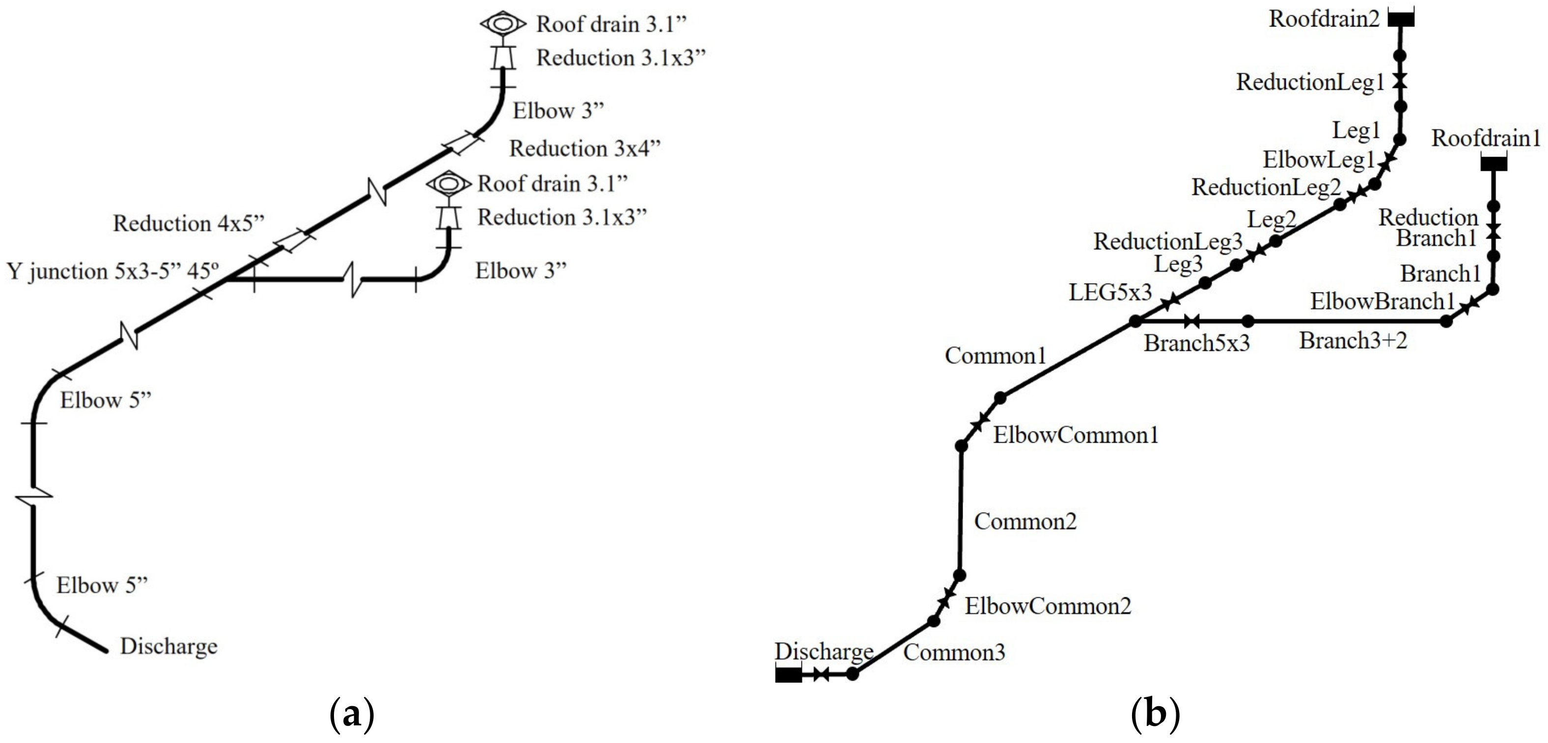
A small installation of an SRDS was analyzed using both software. This system consists, as can be seen in Figure 4, of two siphonic drains that collect rain from two roofs of different size with a single discharge.
The system analysis was performed with both programs. For the EPANET simulation, the individual components (elbows, reductions, unions) were modeled as regulation valves with the same loss coefficient as the real commercial component.
The results of the analysis are shown in Table 5. It can be observed that the flow rate and head values are practically identical in both cases.
It is verified that analysis of complex SRDSs can be performed with EPANET, a free software, with no need to use a specific software developed by manufacturers.
4. Conclusions
Considering the results, it may be concluded that it is possible to use the EPANET to hydraulically analyze SRDSs, although it must be adapted so that the calculation can be carried out. In the same way, it would be possible to size the SRDS using simulation techniques with the EPANET program. It has been verified, by means of a test prototype of an SRDS, that EPANET analysis results are accurate enough.
The errors observed between measurements in the laboratory and the results of the simulation with EPANET are less than 5% for pressures and 3% for flows. These errors improve the results obtained by Arthur and Swaffield [24]. Part of the merit arises from the fact that the minor losses were tested in the laboratory.
In order to perform the analysis with EPANET, it is necessary to modify the conventional data model used for pressure hydraulic networks and define a specific data model for SRDSs.
On the one hand, the discharge point had to be modeled as a node whose demand is not constant but dependent on pressure. On the other hand, the kinetic term of the energy equation had to be added to the data model of each conduction, which, in the conventional model, EPANET data is not considered.
It was verified, through comparison with a specific commercial SRDS analysis software, that EPANET results obtained by means of the simulation model are good enough to consider the analysis as valid.
The error observed between the commercial software and EPANET is negligible.
Due to limitations in the size of the test model used, a roof with a single sump was simulated in the prototype. In future developments, a larger test model will be built to simulate the real behavior of a roof with several sumps.
The result of this work is of great use to engineers as it adds an additional free access tool, widely used at a global level, for the analysis, design, and dimensioning of SRDSs.
Author Contributions
All authors contributed extensively to the work presented in this paper. Conceptualization, G.L.-P., P.L.I.-R., F.J.M.-S. and V.S.F.-M.; data curation, G.L.-P. and P.L.I.-R.; formal analysis, G.L.-P., P.L.I.-R., F.J.M.-S. and V.S.F.-M.; investigation, G.L.-P., P.L.I.-R., F.J.M.-S. and V.S.F.-M.; methodology, G.L.-P., P.L.I.-R. and F.J.M.-S.; resources, G.L.-P., P.L.I.-R., F.J.M.-S. and V.S.F.-M.; software, G.L.-P., P.L.I.-R. and F.J.M.-S.; supervision, G.L.-P., P.L.I.-R., F.J.M.-S. and V.S.F.-M.; validation, G.L.-P., P.L.I.-R., F.J.M.-S. and V.S.F.-M.; visualization, G.L.-P., P.L.I.-R., F.J.M.-S. and V.S.F.-M.; writing—original draft, G.L.-P. and P.L.I.-R.; writing—review and editing, G.L.-P., P.L.I.-R., F.J.M.-S. and V.S.F.-M. All authors have read and agreed to the published version of the manuscript.
Funding
This research received no external funding.
Data Availability Statement
Data sharing not applicable. All data used are included in the text. Detailed raw data are available upon reasonable request.
Conflicts of Interest
The authors declare no conflict of interest.
References
- Gormley, M.; Kelly, D.; Campbell, D.; Xue, Y.; Stewart, C. Building Drainage System Design for Tall Buildings: Current Limitations and Public Health Implications. Buildings 2021, 11, 70. [Google Scholar] [CrossRef]
- May, R.W.P. The Design of Conventional and Siphonic Roof-Drainage Systems. Water Environ. J. 1997, 11, 56–60. [Google Scholar] [CrossRef]
- Arthur, S.; Wright, G.B. Recent and future advances in roof drainage design and performance. Build. Serv. Eng. Res. Technol. 2005, 26, 337–348. [Google Scholar] [CrossRef]
- Fujimura, K.; Sakaue, K. Analysis of pneumatic pressure vibration affected by connecting WCs and discharge load types. Water 2017, 9, 6. [Google Scholar] [CrossRef] [Green Version]
- Arthur, S.; Swaffield, J.A. Siphonic roof drainage: Current understanding. Urban Water 2001, 3, 43–52. [Google Scholar] [CrossRef]
- Escarameia, M.; May, R.W.P. Performance of Siphonic Drainage Systems for Roof Gutters; HR Wallingford: Wallingford, UK, 1996. [Google Scholar]
- Guan, Y.; Fang, Z.; Tang, Z.; Yuan, J. Influence of the vent pipe diameter on the discharge capacity of a circuit vent building drainage system. Build. Serv. Eng. Res. Technol. 2019, 41, 5–24. [Google Scholar] [CrossRef]
- Banisoltan, S.; Rajaratnam, N.; Zhu, D.Z. Experimental and Theoretical Investigation of Vertical Drains with Radial Inflow. J. Hydraul. Eng. 2016, 143, 04016103. [Google Scholar] [CrossRef]
- Arthur, S.; Swaffield, J. Understanding Siphonic Rainwater Drainage Systems. In Proceedings of the CIB W62 Symposium Edinburgh, Water supply and Drainage for Buildings, Edinburgh, UK, 21–23 September 1999; pp. B1/1–B1/16. [Google Scholar]
- Lucke, T.; Beecham, S.; Qu, Y.Y. Estimating Flowrates Through Individual Outlets of Siphonic Roof Drainage Systems. Build. Res. Inf. 2016, 44, 289–300. [Google Scholar] [CrossRef]
- Beattie, R.K.; Jack, L.B. How siphonic roof drainage systems perform in a future climate. In Proceedings of the 2011 Symposium CIB W062, Aveiro, Portugal, 25–28 September 2011; pp. 301–307. [Google Scholar]
- Arthur, S.; Wright, G.B. Siphonic roof drainage systems-priming focused design. Build. Environ. 2007, 2, 2421–2431. [Google Scholar] [CrossRef]
- Lucke, T.; Arthur, S. Plastic pipe pressures in siphonic roof drainage systems. Build. Res. Inf. 2011, 39, 79–92. [Google Scholar] [CrossRef]
- Geberit Verwaltungs AG, Geberit Proplanner. Available online: https://www.geberit-global.com/planning-installation/geberit-proplanner/ (accessed on 25 May 2023).
- R. M. S. (RMS), SiphoniTec® Siphonic Roof Drain Sizing Software Information. Available online: https://www.jrsmith.com/siphonitec-siphonic-roof-drain-sizing-software-information (accessed on 25 May 2023).
- Siphonix Worldwide Ltd. Roof Drainge System. Available online: http://www.siphonix.com/software.html (accessed on 25 May 2023).
- Saint Gobain PAM. EPAMS Software. Available online: https://www.pam-drainage-solutions.com/rainwater-epams (accessed on 25 May 2023).
- Roland, R.E. Geberit ProPlanner 2020—Roof Drainage Systems; Training Manual; Geberit International AG: Rapperswil, Switzerland, 2020. [Google Scholar]
- Brkicbrkic, D. Iterative Methods for Looped Network Pipeline Calculation. Water Resour. Manag. 2011, 25, 2951–2987. [Google Scholar] [CrossRef] [Green Version]
- Wright, G.B.; Swaffield, J.A.; Arthur, S. Investigation into the performance characteristics of multi-outlet siphonic roof drainage systems. In Global Solutions for Urban Drainage; American Society of Civil Engineers: Reston, VA, USA, 2002; pp. 1–16. [Google Scholar] [CrossRef] [Green Version]
- Rossman, L. EPANET 2.0 Users Manual; U.S. Environmental Protection Agency: Washington, DC, USA, 2000.
- Chaudhry, M.H. Open-Channel Flow, 2nd ed.; Springer: New York, NY, USA, 2008. [Google Scholar]
- Todini, E.; Pilati, S. A gradient algorithm for the analysis of pipe networks. In Computer Applications in Water Supply: Volume 1—Systems Analysis and Simulation; Coulbeck, B., Orr, C.-H., Eds.; John Wiley & Sons: Hoboken, NJ, USA, 1988; pp. 1–20. [Google Scholar]
- Arthur, S.; Swaffield, J.A. Siphonic roof drainage system analysis utilising unsteady flow theory. Build. Environ. 2001, 36, 939–948. [Google Scholar] [CrossRef]
- May, R.W.P. Design Criteria for Siphonic Roof Drainage Systems; Report SR654; HR Wallingford: Wallingford, UK, 2004. [Google Scholar]
- Idelchik, I.E. Handbook of Hydraulic Resistance, 3rd ed.; Begell House Inc.: New York, NY, USA, 1996. [Google Scholar]
Figure 1.
Laboratory SRDS small-size test model.
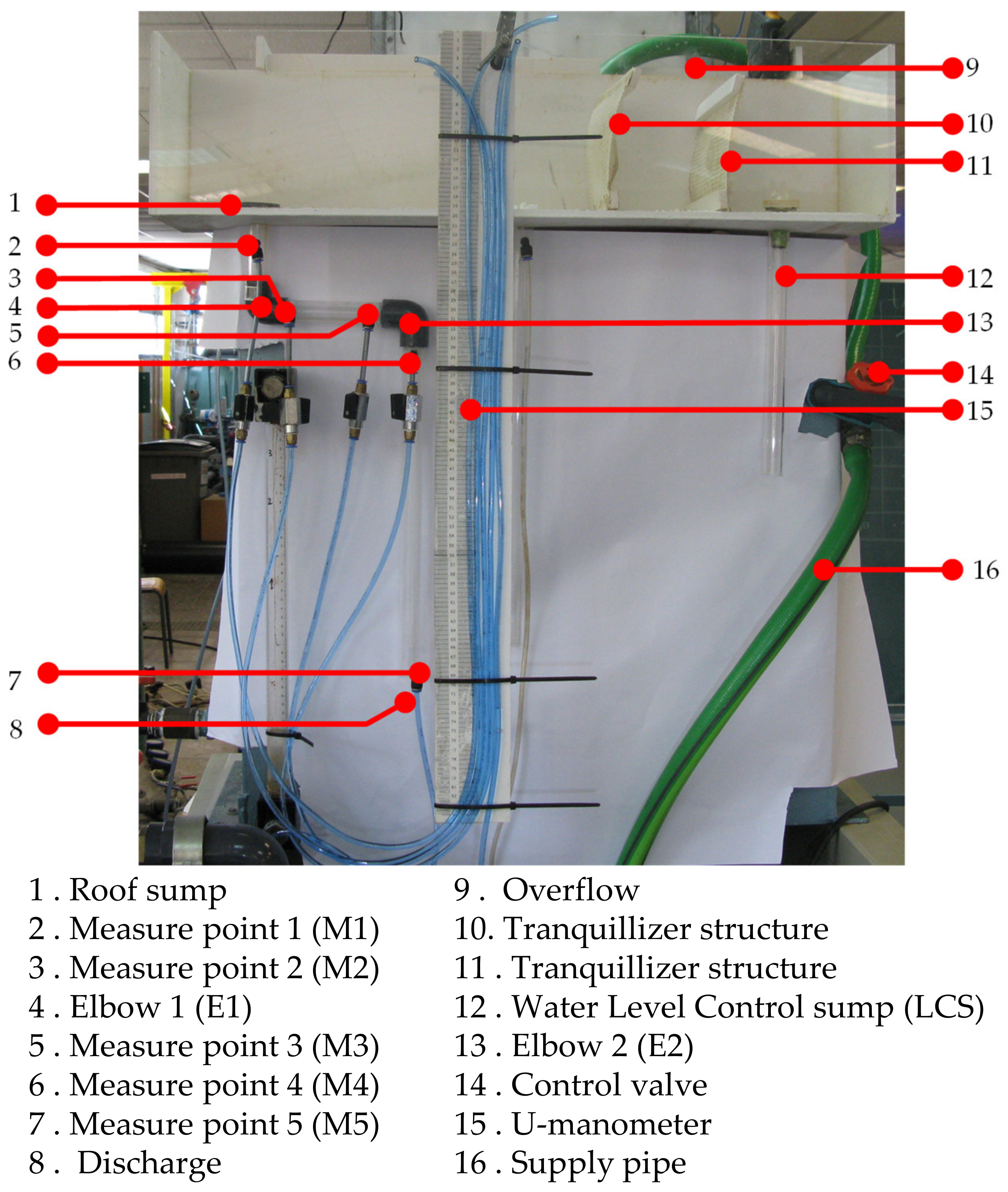
Figure 2.
EPANET model.
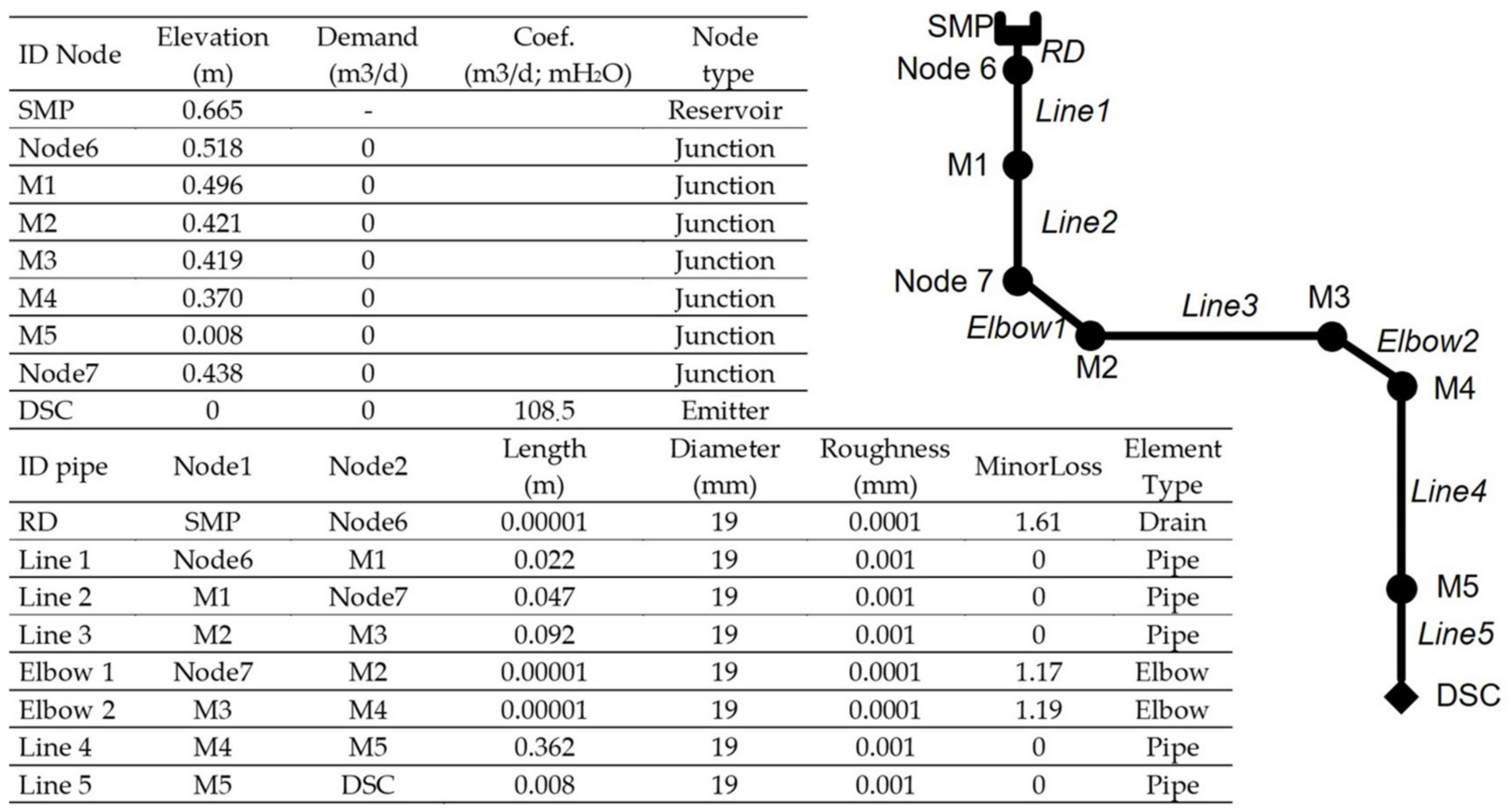
Figure 3.
Real flow measure vs. EPANET flow for each series of measurements. In this figure, each blue circle corresponds to a test in Table 2.
Figure 3.
Real flow measure vs. EPANET flow for each series of measurements. In this figure, each blue circle corresponds to a test in Table 2.
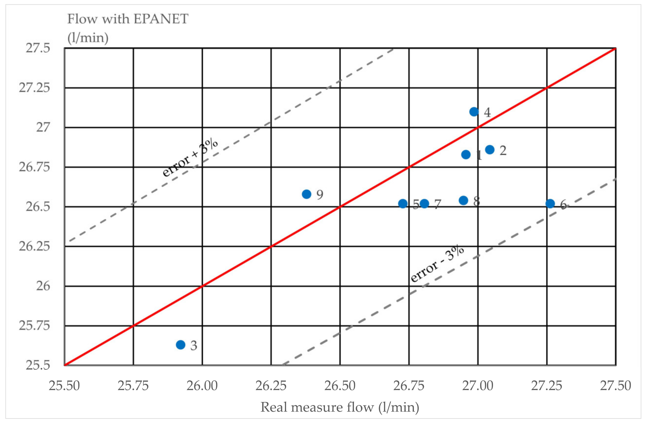
Figure 4.
(a) SRDS model in SIPHONITEC®. (b) SRDS model in EPANET.

Table 1.
Water level, pressure reading, and drain flow for each test.
| Test | 1 | 2 | 3 | 4 | 5 | 6 | 7 | 8 | 9 |
|---|---|---|---|---|---|---|---|---|---|
| Water level (mm) | −68 | −67 | −124 | −55 | −83 | −83 | −83 | −82 | −80 |
| PM1 (mmwc) | −417 | −415 | −431 | −414 | −407 | −410 | −405 | −405 | −417 |
| PM2 (mmwc) | −572 | −573 | −577 | −563 | −561 | −557 | −562 | −563 | −558 |
| PM3 (mmwc) | −580 | −580 | −579 | −570 | −567 | −566 | −569 | −567 | −566 |
| PM4 (mmwc) | −724 | −724 | −723 | −722 | −722 | −722 | −722 | −723 | −724 |
| PM5 (mmwc) | −761 | −774 | −765 | −765 | −765 | −766 | −765 | −766 | −770 |
| Q (l/min) | 26.96 | 27.04 | 25.92 | 26.99 | 26.73 | 27.26 | 26.81 | 26.95 | 26.38 |
Table 2.
Coefficients ki of head loss for a D = 19·10−3 m pipe. Dimensionless.
| Element | 1 | 2 | 3 | 4 | 5 | 6 | 7 | 8 | 9 | Mean |
|---|---|---|---|---|---|---|---|---|---|---|
| Roof sump | 1.71 | 1.68 | 1.57 | 1.78 | 1.56 | 1.48 | 1.52 | 1.51 | 1.73 | 1.61 |
| Elbow 1 | 1.17 | 1.18 | 1.19 | 1.12 | 1.18 | 1.08 | 1.20 | 1.19 | 1.10 | 1.17 |
| Elbow 2 | 1.13 | 1.12 | 1.22 | 1.19 | 1.23 | 1.20 | 1.20 | 1.22 | 1.23 | 1.19 |
| Discharge | 0.06 | −0.04 | 0.00 | 0.03 | 0.02 | 0.03 | 0.02 | 0.02 | −0.03 | 0.00 |
Table 3.
EPANET analysis results for total pressure, dynamic pressure, and static pressure.
| Intake | PEPANET (Pa) | Pd (Pa) | Ps (Pa) |
|---|---|---|---|
| M1 | −216 | 1599 | −1814 |
| M2 | −932 | 1599 | −2531 |
| M3 | −1040 | 1599 | −2639 |
| M4 | −1942 | 1599 | −3541 |
| M5 | 1089 | 1599 | −510 |
Table 4.
Static pressure from the analysis with EPANET vs. real measure.
| Intake | Ps,EPANET (Pa) | Ps,real (Pa) | Error (%) |
|---|---|---|---|
| M1 | −1814 | −1864 | 2.7 |
| M2 | −2531 | −2589 | 2.3 |
| M3 | −2639 | −2639 | 0.0 |
| M4 | −3541 | −3650 | 3.1 |
| M5 | −510 | −520 | 2.0 |
Table 5.
Results of the simulation for node head.
| SIPHONITEC Results | EPANET Results | |||||
|---|---|---|---|---|---|---|
| Flow (cfs) | Head in (ftwc) | Head out (ftwc) | Flow (cfs) | Head in (ftwc) | Head out (ftwc) | |
| Discharge | 1.634 | 2.342 | 0.000 | 1.637 | 2.350 | 0.000 |
| Common3 | 1.634 | 3.714 | 2.342 | 1.637 | 3.720 | 2.350 |
| ElbowCommon2 | 1.634 | 4.159 | 3.714 | 1.637 | 4.160 | 3.720 |
| Common2 | 1.634 | 6.490 | 4.159 | 1.637 | 6.490 | 4.160 |
| ElbowCommon1 | 1.634 | 6.799 | 6.490 | 1.637 | 6.800 | 6.490 |
| Common1 | 1.634 | 10.776 | 6.799 | 1.637 | 10.770 | 6.800 |
| LEG5x3 | 0.690 | 9.621 | 10.776 | 0.693 | 9.600 | 10.770 |
| Leg3 | 0.690 | 9.646 | 9.621 | 0.693 | 9.630 | 9.600 |
| ReductionLeg3 | 0.690 | 9.926 | 9.646 | 0.693 | 9.910 | 9.630 |
| Leg2 | 0.690 | 12.285 | 9.926 | 0.693 | 12.270 | 9.910 |
| ReductionLeg2 | 0.690 | 13.007 | 12.285 | 0.693 | 13.000 | 12.270 |
| ElbowLeg1 | 0.690 | 13.979 | 13.007 | 0.693 | 13.970 | 13.000 |
| Leg1 | 0.690 | 14.706 | 13.979 | 0.693 | 14.700 | 13.970 |
| ReductionLeg1 | 0.690 | 14.818 | 14.706 | 0.693 | 14.820 | 14.700 |
| RoofDrain2 | 0.690 | 15.267 | 14.818 | 0.693 | 15.270 | 14.820 |
| Branch5x3 | 0.944 | 15.269 | 10.776 | 0.944 | 15.280 | 10.770 |
| Branch3+2 | 0.944 | 16.691 | 15.269 | 0.944 | 16.700 | 15.280 |
| ElbowBranch1 | 0.944 | 18.511 | 16.691 | 0.944 | 18.520 | 16.700 |
| Branch1 | 0.944 | 19.866 | 18.511 | 0.944 | 19.870 | 18.520 |
| ReductionBranch1 | 0.944 | 20.075 | 19.866 | 0.944 | 20.080 | 19.870 |
| RoofDrain1 | 0.944 | 20.916 | 20.075 | 0.944 | 20.920 | 20.080 |
Disclaimer/Publisher’s Note: The statements, opinions and data contained in all publications are solely those of the individual author(s) and contributor(s) and not of MDPI and/or the editor(s). MDPI and/or the editor(s) disclaim responsibility for any injury to people or property resulting from any ideas, methods, instructions or products referred to in the content. |
© 2023 by the authors. Licensee MDPI, Basel, Switzerland. This article is an open access article distributed under the terms and conditions of the Creative Commons Attribution (CC BY) license (https://creativecommons.org/licenses/by/4.0/).
Share and Cite
MDPI and ACS Style
López-Patiño, G.; Iglesias-Rey, P.L.; Martínez-Solano, F.J.; Fuertes-Miquel, V.S. Analysis of Siphonic Roof Drainage Systems with EPANET. Environments 2023, 10, 123. https://doi.org/10.3390/environments10070123
AMA Style
López-Patiño G, Iglesias-Rey PL, Martínez-Solano FJ, Fuertes-Miquel VS. Analysis of Siphonic Roof Drainage Systems with EPANET. Environments. 2023; 10(7):123. https://doi.org/10.3390/environments10070123
Chicago/Turabian StyleLópez-Patiño, Gonzalo, Pedro L. Iglesias-Rey, Francisco Javier Martínez-Solano, and Vicente S. Fuertes-Miquel. 2023. "Analysis of Siphonic Roof Drainage Systems with EPANET" Environments 10, no. 7: 123. https://doi.org/10.3390/environments10070123
Note that from the first issue of 2016, this journal uses article numbers instead of page numbers. See further details here.