
Accumulative Heat Stress in Ruminants at the Regional Scale under Changing Environmental Conditions

1
Department of Environment and Primary Industries, Parkville, VIC 3052, Australia
2
School of Engineering, University of Melbourne, Parkville, VIC 3010, Australia
3
Faculty of Science, University of Melbourne, Parkville, VIC 3010, Australia
*
Author to whom correspondence should be addressed.
†
Current address: Independent Researcher, København 2500, Hovedstaden, Denmark.
Environments 2024, 11(3), 55; https://doi.org/10.3390/environments11030055
Submission received: 16 January 2024
/
Revised: 4 March 2024
/
Accepted: 6 March 2024
/
Published: 14 March 2024
Abstract
:Environmental heat stress is implicated in various animal health issues in ruminants, including reproduction rates, mortality rates, and animal physical quality. During extremely hot weather, there is often no overnight equilibration of animal temperature with its cooling effect, and the accumulated heat load becomes an important factor in animal health for ruminants such as sheep. Using the heat load index (HLI), a heat load model is used as an indicator of heat stress on an hourly basis and annually, using downscaling models for temperature, humidity, solar radiation, and wind speed, in both spatial and temporal cases, across several example sites in regional Victoria. Analysis is provided on the performance of the downscaling models and various adaptation and mitigation options are discussed and tested. These options include using different tree planting patterns to modify solar radiation exposure and wind effects, with mixed results because adding shading structures may also diminish the effect of wind-based cooling. The modelling experiments indicated that (1) heat stress is likely to increase under future climate conditions and could represent a serious threat to the health of small ruminants; (2) adaptation measures by means of tree planting to provide shade may not be sufficient to alleviate projected heat stress; and (3) other adaptation measures will need to be considered. Indicative results for heat stress under potential future environments are provided for 2030, 2050, and 2070. Also discussed is the performance of wind speed modelling, and the effect of heat stress on animal growth and ram fertility.
1. Introduction
In addition to premature mortality, exposure of ruminants to heat stress has many other consequences, including decreasing animal welfare, lower quality of milk and wool, and health issues such as weight loss, lower reproduction rates, and chronic diseases. In an early study, it was noted that environmental stressors can lead to a heat stress response that includes raised body temperature and depression of the metabolic rate and lower appetite [1]. The heat load on the animal is decreased by the action of panting and sweating. Heat load can also be decreased via the adoption of environmental control factors, including shading effects due to the use of planted trees or artificial shading structures.
The effect of heat stress on ruminants has been the subject of increasing research due to animal welfare issues and possible losses in rural production. The effect on productivity is important during the summer months in hotter climate scenarios and landscapes, where overnight cooling is not possible. Various spatial–statistical modelling approaches to heat stress in outdoor conditions have been investigated in the past, and the current study represents a further extension in this line of research [2,3,4,5].
Pioneering research was carried out in temperature control in cattle by Finch [6], and associated research in nutritional strategies by Beede and Collier [7]. Further work on the problem of heat stress in cattle has been reported by others [8,9,10,11,12]. In recent years, significant research in the development of predictive models for heat stress indicators has been conducted for large ruminants, such as cows, and by the dairy and beef cattle industries, particularly in northern Australia (see Gaughan et al. [2,13,14]).
In the case of small ruminants, such as sheep, recent reviews have covered the negative effect of heat stress on metabolic activity, behaviour, and reproductive success for rams (see, for example, Sierra et al. [15] and van Wettere [16]), who have highlighted reports of low seminal quality (motility, sperm abnormalities, concentration, DNA damage, and lower ejaculate volume) and libido. The impact of heat stress has also been documented for the fertility of ewes (oestrus cycle duration, ovulation rate, oocyte quality, and embryo loss), embryo development, birth weight, and lactation [16]. This latter research extends the knowledge acquired by historical studies on heat stress in sheep.
However, while the impact of exposure to heat stressors has been relatively well documented (from limited work in environmental chambers or measurements taken after sporadic heat treatment or heat waves), the actual combination of factors that triggers negative responses has not been systematically explored for predicting the occurrence and impact of heat stress on sheep. While some authors have reported ranges of temperatures where the effect of heat stress was measured, ranging between 29 and 50 °C, the combination of factors that influence heat stress (such as solar radiation, relative humidity, wind speed, etc.) makes the use of temperature only as an indicator of heat stress impractical and prone to uncertainty (except for indoor use together with relative humidity [2,4]).
Historical work in heat stress and its effect on animals has been largely centred around the issue of the effects of heat stressors on physiology and biochemistry, with attention also devoted to the energy balance outdoors [1,2,4]. Silanikove [1] suggested in an early study an energy balance equation with multiple inputs from the environment. There was some early recognition of the potential for mathematical models for future growth and spatial analysis for regional analysis of agricultural data, but sufficient data points were lacking at that time for more advanced computer analysis for grazing animals [3,5].
Stressors can arise from external events, such as increased temperature and humidity, and can lead to a stress response in the sheep which can be behavioural, physiological, or immunological in nature, resulting in a state of heat stress. Previous predictive models for heat stress assessment for grazing animals were typified by the so-called temperature–humidity index (THI), which is an indicator of thermal stress and is widely used in the dairy and beef industries [4]. It is also used to estimate the degree of thermal stress experienced by sheep.
More recently, it became apparent that heat load in the field based on temperature and humidity using the THI model as an indicator may be unduly restrictive because it fails to take into account other external uncontrolled variables, such as solar radiation and wind speed, which can vary greatly in outdoor environments [12]. Eigenberg et al. [14] reported that temperature and humidity accounted for only about 50% of external heat stressors, with the remainder due mainly to solar radiation and wind speed. As an indicator of outdoor heat stress, the heat load index (HLI) is now used more widely than the THI [2]. The THI model nevertheless still has applications for enclosed environments, such as sea export of live sheep [17].
The HLI model provided a key enhancement over the THI by adding the significant variables of solar radiation and wind speed. The model was extended to the situation where overnight equilibration of heat load was not possible, i.e., temperatures did not fall sufficiently to allow heat dissipation, by defining the associated accumulated heat load (AHL), which was based on integration of the HLI over a defined time period. The AHL is also referred to as the accumulated heat index (AHI).
Application of the HLI appears to be gradually replacing the THI as a metric for heat stress in the cattle industry [2,8,10]. It is also being used as a model for predictions involving sheep response to heat stress, subject to different HLI boundary conditions (e.g., see Stockman, [17]. An additional issue of importance is the spatial variability of the heat stress index, which has received little attention in the research literature. Coupled with a map of climate change scenarios, this additional modelling step provides more information for regional studies of heat stress—especially in the context of the spatial analysis of the components of rural production systems and their optimisation under environmental constraints [18].
The effect of heat stress on lamb growth and weight gain has also been the subject of considerable attention, for example, see the seminal work by Ames and Brink [19] and others [20,21]. Growth models often require fitting by regression methods to a pre-defined non-linear model, such as a power function, Gompertz model, or various dose–response models [20,21,22,23]. The growth models are often monotonically increasing with lamb age, whilst at other times there is a roll-off after adulthood is reached, especially after the effect of heat stress [19,24]. Growth may also be affected by breed and genetics and some studies have investigated genetic differences using random regression methods, such as exponential, logistic, and linear mixed effects models [20,21,24].
Heat stress can also affect fertility in sheep, especially with respect to rams, where scrotum temperature rises with ambient temperature and heat stress. Higher scrotum temperature is associated with lower sperm counts and therefore lower conception rates in periods of high temperature and heat stress [25]. Research has investigated the link between semen degeneration and temperature of the scrotum; see, for example, Moule and Waites [25]. A comprehensive early review on physiological traits and heat stress was conducted by Marai et al. [26].
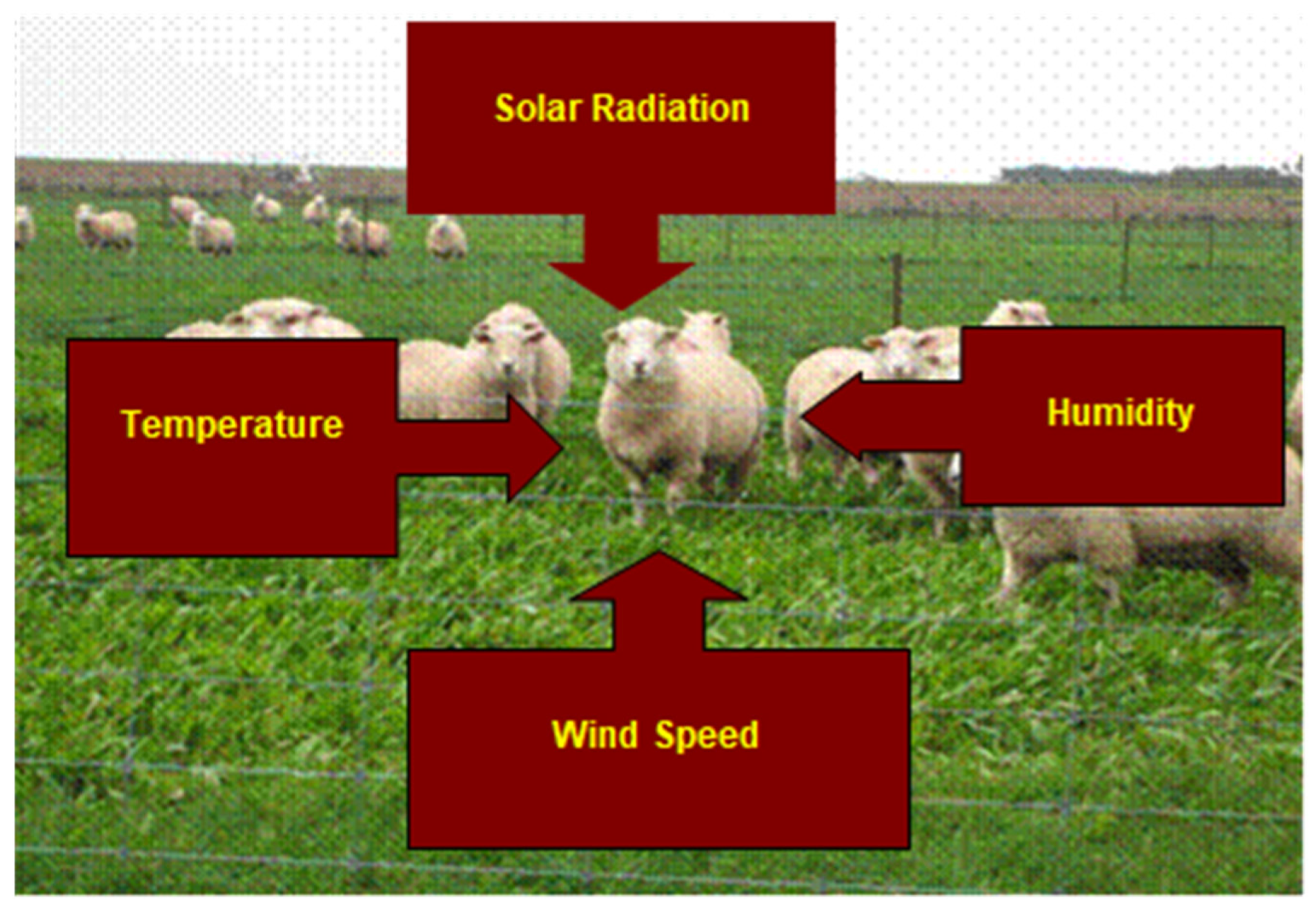
External environmental factors that can cause heat stress in sheep are shown in Figure 1. Solar radiation was recognised by Papanastasiou [27], suggesting the need for the future development of a model for sheep that provides information on heat flows.
Recent research on heat stress in small ruminants such as sheep relates mostly to physiology and biochemistry, and to the development of heat stress thresholds in sheep [28,29,30,31,32]. There appears to be very little recent research reported on the effect of overnight cooling and the modelling of accumulative heat load in the face of severe (hot) environmental conditions or climate change.
The aim of this study was to investigate accumulative heat stress due to environmental conditions at a regional level, and possible adaptation and mitigation strategies for sheep in the state of Victoria in Australia. This study involved investigation of the wind speed modelling and downscaling approaches necessary to convert inputs to hourly data and produce results on an annual basis. The effects of heat stress on weight gain and ram fertility were explored in the context of the accumulative heat load model. The analysis required the downscaling of monthly data for temperature, humidity, solar radiation, and wind speed. The data from Victoria were used to develop a regression model for wind speed based on the Weibull probability distribution. This study explored the potential benefit of farm management options, such as tree planting and shading infrastructure, and the implications of future climate change.
2. Materials and Methods
2.1. Calculation of Heat Stress Indicators
Thermal stress in cattle and other ruminants can be modelled through a series of indicators often related to animal physical status such as panting rates. To identify heat stress from climate variables, we calculated the heat load index HLI and the AHI based on the following model formulas. Some other approaches use only temperature and relative humidity, but thresholds are similar at around 25 °C. This is when sheep wellbeing begins to be seriously affected, with some variability between different breeds [32]. The upper critical temperature for sheep is 31 °C (for more details see van Wettere [16]).
2.1.1. Heat Load Index (HI)
The heat load index (HLI) was calculated based on the conditional statement defined by Gaughan et al. [2], where
IF BGT < 25 °C THEN
IF BGT > 25 °C THEN
where BGT is the black globe temperature, BGT (°C), RH is the relative humidity, RH (%), and WIND is the wind speed at a height of 2 m in units of ms−1.
2.1.2. Accumulated Heat Load Index AHI
The accumulated heat load index (AHI) refers to the accumulative AHL over a time period. It is also referred to in the literature as the accumulated heat load (AHL) model and is based on the following conditional logic statements, adapted, assuming hourly temperature measures, from the approach reported by Gaughan et al. [2]:
where i corresponds to the time of day (in hours) and Acci corresponds to the hourly heat stress accumulation, where
The HLI heat stress thresholds (HLIlow and HLIhigh) are associated with the type of ruminant under consideration, e.g., cattle or sheep. It is noteworthy that
- (a)
- Acc cannot fall below zero > 0 (0 indicating an animal in thermal balance) between two consecutive time steps.
- (b)
- In this application, we used Gaughan’s heat stress reference thresholds of HLIlow = 77 and HLIhigh = 86.
- (c)
- Accumulated heat load decreases in the evening to return to zero at night.
The calculation of the HLI and AHL requires the use of hourly inputs. To derive hourly inputs for Tmin, Tmax, RHMin, RHMax, Rad, and Wind data from daily and monthly values (for WIND), we performed a temporal downscaling using the set of methods described below.
2.2. Downscaling Daily to Hourly Data
Predictions from a model gained at a coarse resolution can be interpolated at a finer scale using a process known as downscaling [34]. The estimation of hourly temperatures from daily temperatures is possible by using various numerical and statistical techniques.
2.2.1. Downscaling Temperature
We initially compared two methods of downscaling daily temperature to hourly, one proposed by Darbyshire et al. [35] and the other by Chow and Levermore [36]:
- Method 1: Proposed by Darbyshire et al. [35]
This temperature downscaling method is based on consideration of a nighttime temperature, Tn, and a daytime temperature, Td, calculated as a function of day length DL, the daily maximum Tmax and minimum Tmin temperature, and time of day (in hours), t.
- Day length, DL, was calculated as follows (Darbyshire et al. [35]):
- = latitude (decimal degrees)
- where dn = the day number relative to 1 January.
The time of lowest temperature (sunrise), tmin was defined by the following relationship with day length,
This is used in the calculation of daytime temperature for each hour Tt based on the following relationships,
where
- Tt = temperature for time t.
- Td = daytime temperature.
- Tn = nighttime temperature.
Daytime temperature is calculated as follows:
The night-time temperature time series is given by
Subject to
where
- Ts = temperature at sunset.
- Method 2: CBSE Proposed by Chow and Levermore [36]
In the proposed CBSE linking method [36], estimation of temperature, T, at time t is based on the relationship with the previous temperature, Tprev, and following temperature Tnext, i.e.,
subject to
where
- t = time of day in hours.
- tmax = time when maximum temperature occurs.
- tmin = time when minimum temperature occurs.
- tprev = time when the previous temperature is considered.
- tnext = time when the next temperature is considered.
- T*min = minimum temperature Tmin of the next day.
2.2.2. Comparison of Two Approaches to Downscaling Temperature
The effectiveness of both approaches to replicate field temperatures was compared using hourly data records from two regional sites in Victoria (Hamilton and Tatura) from 1 January 2005 to 10 September 2010 for Hamilton and from 1 January 2005 to 2012 for Tatura. The results from this study, detailed in Table 1, indicated that Method 2 (R2 = 0.894) consistently produced a better estimation than Method 1 (R2 = 0.8469) for both sites. Method 2 was therefore subsequently used to downscale hourly data from daily inputs.
2.2.3. Downscaling Relative Humidity
We assumed that relative humidity could be downscaled using an approach similar to that used for temperature (since both a daily maximum and minimum were available) and we applied the same equations (Method 2) to downscale relative humidity from RHmin and RHmax, accounting for the fact that RHmin occurred in tandem with solar noon (Tmax) and RHmax at sunrise (Tmin).
2.2.4. Downscaling Solar Radiation
The daily solar radiation was downscaled in the model through the following approach, illustrated in Figure 2:
First, we estimated maximum daily solar radiation RadMax from the cumulated solar radiation values (provided by CATCLIM and SILO, see [37]) based on the following calculations.
where
- t = time of day (1 to 24 h).
- tsunrise = time at sunrise, where
- tsunset = time at sunset, where
- tRadmax= time at which maximum radiation occurs (12 + 1).
- DL = day length as defined previously.
We assumed hourly solar radiation follows a sinusoidal function during daytime and is equal to zero during nighttime, and radiation at a time t was estimated by
2.2.5. Downscaling of Wind Data
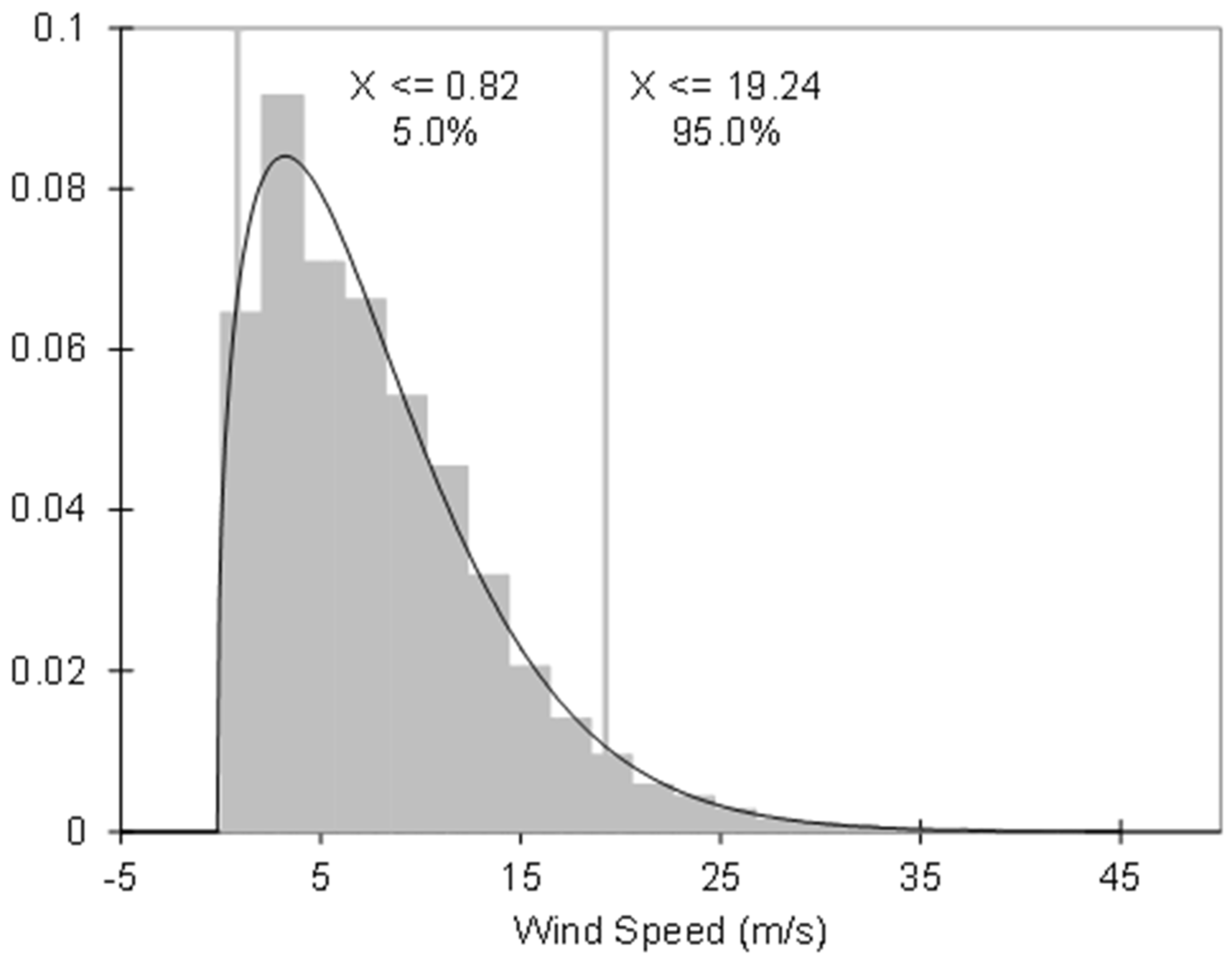
Wind speed was treated as a stochastic process that can be modelled by a probability distribution. Previous studies in Europe and elsewhere have suggested that a suitable random distribution of best fit may be the Weibull distribution [38,39]. The Weibull probability density function (PDF) [40], illustrated in Figure 3, provides basic stochastic input for surface wind speeds for use in a probabilistic simulation for the HLI and AHL models.
In the current study, extensive data from the experimental farm at Hamilton in Victoria was accessed and modelled using the Weibull PDF,
where the defining parameters α and β are estimated from regression analysis from empirical data. The cumulative distribution function (CDF) is given by the following:
The Weibull random variable, W, can be computed from the uniform random variable, R, using the following expression:
where R is the random variable from a uniform distribution. The median value for the Weibull distribution, which is usually skewed, is given by
The Weibull random variable used to populate hourly wind speed data was fitted to Hamilton hourly data for 2010 by least squares regression analysis. From this analysis, we estimated α = 1.37368643864572 and β as the monthly average wind value. Applying this random distribution to all locations across the state, on a 0.05-degree grid, we assumed α as constant and β as the monthly average for this location obtained from the OzClim database [41].
2.3. Accuracy of Downscaling Approach
The accuracy of the above defined downscaling approaches was estimated by comparing actual versus modelled outputs for each of the considered climatic variables, making use of hourly climate records for the location of Hamilton, Victoria (from 1 January 2005 to 10 September 2010). The results, presented in Table 2, indicate good levels of confidence (>85%) for temperature, solar radiation, and wind speed.
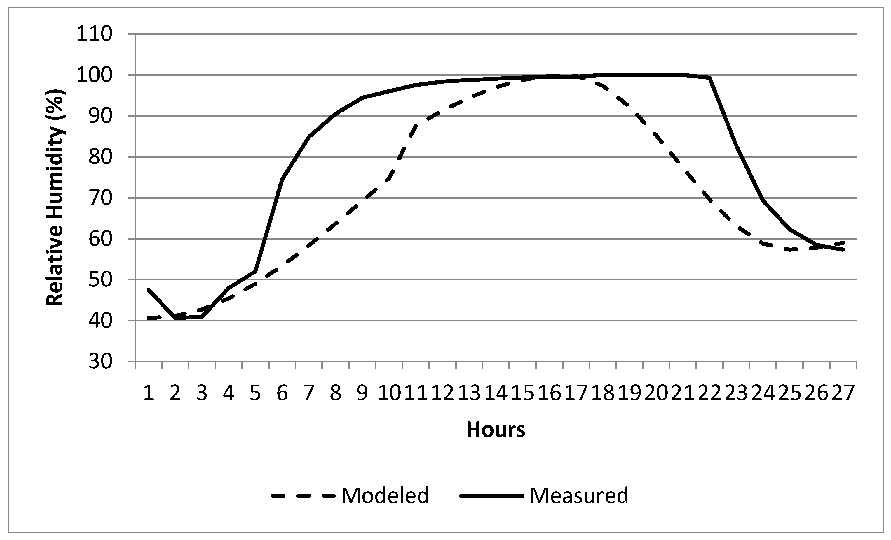
Lower levels of confidence (70%) were obtained for relative humidity. This discrepancy between modelled and measured relative humidity can be explained by the fact that on rainy days (when the atmosphere is saturated with water), variations in relative humidity do not follow a sinusoidal pattern, but rather plateau during the whole rain period (see Figure 4). As our study focused on heat stress, this discrepancy may be a minor issue, as in Victoria hot days are typically associated with dry spells rather than rain; see [42]. This, however, could be an issue if our approach was to be applied to wetter, hotter climates.
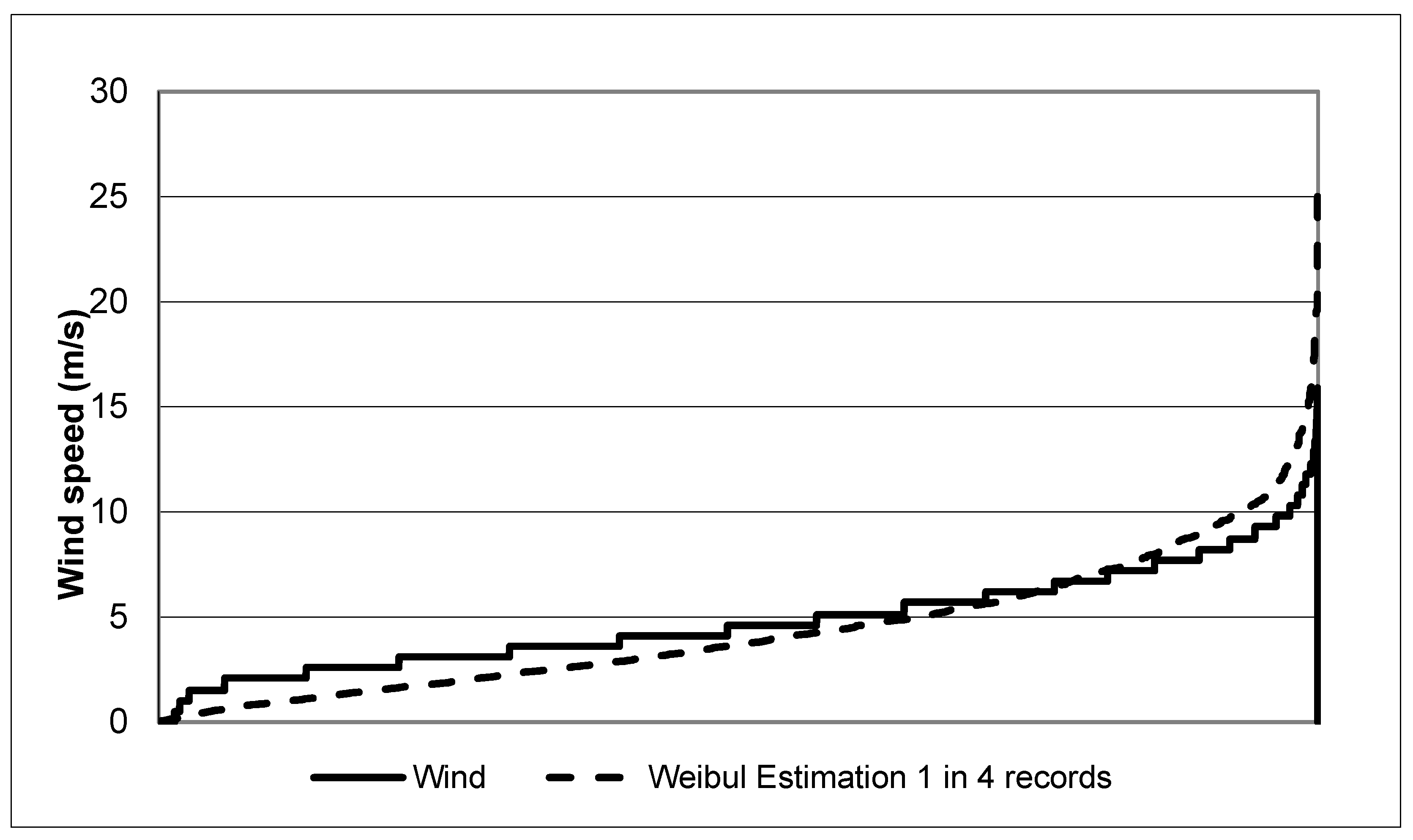
The R2 results for the wind parameter were obtained by ordering the outputs (6060 records) of our Weibull distribution and comparing them with the ordered measured data for the same duration (Figure 5).
These results indicate that the Weibull distribution provides a good estimation of the variability associated with wind variations. However, since this distribution is based on a random function, it cannot provide an estimation of measured wind data on an hour-by- hour basis. Rather, running multiple instances for the same location and time can provide us with a sample of the potential distribution that could be expected for this location.
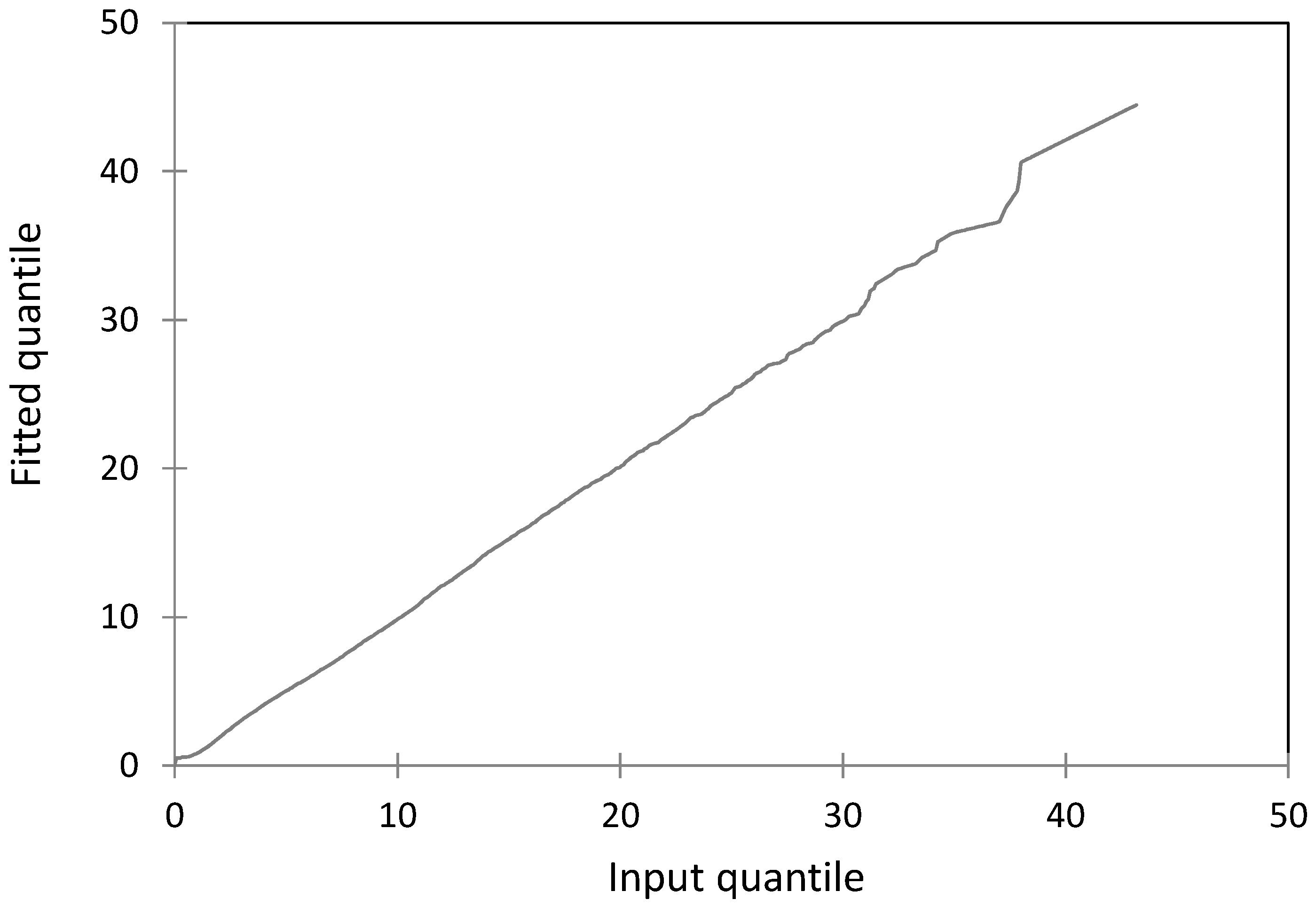
The Q–Q plot for the wind speed data fitted to the Weibull distribution is depicted in Figure 6, indicating a good fit between experimental and theoretical distributions. The Q–Q plot compares the probability distribution of the dataset with that of the model predictions, i.e., it compares the plotting of quantiles in one distribution to those in the other (and is analogous to comparing histograms, but more graphically informative). When the distributions are similar, the Q–Q plot will follow a straight line. When the distributions are linearly related, the points will follow a straight line but not necessarily at an angle of 45 deg. This is a non-parametric approach for comparing distributions for goodness-of-fit and does not require values for paired data arranged in a scatter plot. In the latter case, a plot at each time step of wind speed observed (m/s) against wind speed predicted showed a coefficient of determination of R2 = 0.99, which was statistically significant at the 0.01 level of significance (los).
Observations from the Hamilton hourly data indicated that wind changes did not occur on an hourly basis but rather in four-hour blocks. We therefore used every fourth value from the hourly wind speed values generated from the probability distribution.
The generation of hourly wind data was based on the Weibull distribution. In order to appropriately sample this distribution and obtain an accurate representation of possible variations, each simulation was repeated across multiple iterations > 100 as computed using Equation (31).
The number of iterations, n, required for the probabilistic simulation of HLI was estimated from sampling theory according to the following,
where the standard deviation, σ, is estimated from a short sample run, e.g., of n = 100 iterations for the specified error, ε, in the mean value (Freund [23]). The assumptions are that the errors are normally distributed, and the analysis is based on sampling theory for the 95% confidence interval (CI).
For estimation of HLI, a trial simulation of 100 iterations indicated that, given the magnitude of the sample variance, the 95% confidence interval for n = 100 iterations in the Monte Carlo simulation would be subject to an error in the mean result of less than ε = 2%. The mean and standard deviation were estimated from samples of daily data.
2.4. Climate Data
Our modelling approach made use of a combination of historical and projected climate datasets covering the state of Victoria, at a resolution of 0.05 degrees.
Historical daily records (from 1935 to 1990) of minimum temperature (Tmin), maximum temperature (Tmax), minimum relative humidity (RHMin), maximum relative humidity (RHMax), and solar radiation (Rad) (see Table 3) were sourced from the former Queensland Department of Natural Resources and Environment ‘SILO’ data service [43].
Daily climate projections of Tmin, Tmax, RHmin, RHmax, and Rad, relative to the years 2030, 2050, and 2070, were generated by the Catchment Analysis Toolkit Climate Change Module (CATCLIM), following a methodology previously described by Weeks at al [37]. This procedure generated a set of 56 years for each climate change scenario year (2030, 2050, and 2070), by applying de-trended daily “weather” variability observed during the years 1935 to 1990 to IPCC projections of monthly climate data. This method was chosen because it provides present day annual variability for each of the three future years consistent with IPCC projections. In interpreting these projections, there is no annual progression towards these years with the assumption that each of the future years are representative of the expected climate. For more details, refer to [37]. Daily climate projections were produced for the SRES Marker Scenario A1FI, using the CSIRO Climate Model Mk 3.5, with a moderate rate of global warming [44,45].
Projections of daily wind data could not be generated with this approach as the SILO records do not include this data. Projections of monthly average wind speed were obtained from the OzClim web-based tool for the years 2030, 2050, and 2070, and data for the year 1990 (baseline) were obtained by substituting the “changes from baseline in 2030” to 2030 predictions [41]. These monthly average wind data were then used to generate hourly downscaling using a Weibull probability distribution [40].
2.5. Computational Methods
A software package was developed, composed of Python scripts, making use of the package for scientific computing, Python 2.7 ‘Numpy’ (see http://www.numpy.org/ accessed on 15 January 2024). Output files were then imported and visualised in ESRI ArcGIS 10.0 and final data analysis was performed using Microsoft Excel 2010. The following tasks were performed:
- Data formatting: compiling input data (*.asc files) for each day, variable, and location into a series of yearly arrays combining 365 or 366 elements (for leap years).
- Hourly downscaling and index calculation: calculating hourly values for Tmax, TMin, RHmax, RHmin, Rad, and Wind, as described by Equations (5)–(24), deriving from these values the HLI and AHL indices, described by Equations (1)–(4). Three AHL values were recorded hourly, (a) daily maximum AHL (peak), (b) cumulative daily AHL at time 00:00, providing information on whether night cooling was sufficient to alleviate heat stress, and (c) time (in hours) during which animals were continuously exposed to heat stress (AHL > 0).
- Summary across years and iterations: creating maximum, minimum, average, and standard deviation summary values for each variable and location across all 56 possible futures associated to each climate change scenario year and each iteration of the model (sampling of the Weibull distribution).
- Regionalisation: summarising results across broad geographical locations rather than for each single point of the 0.05-degree Victorian grid.
2.6. Management Scenarios
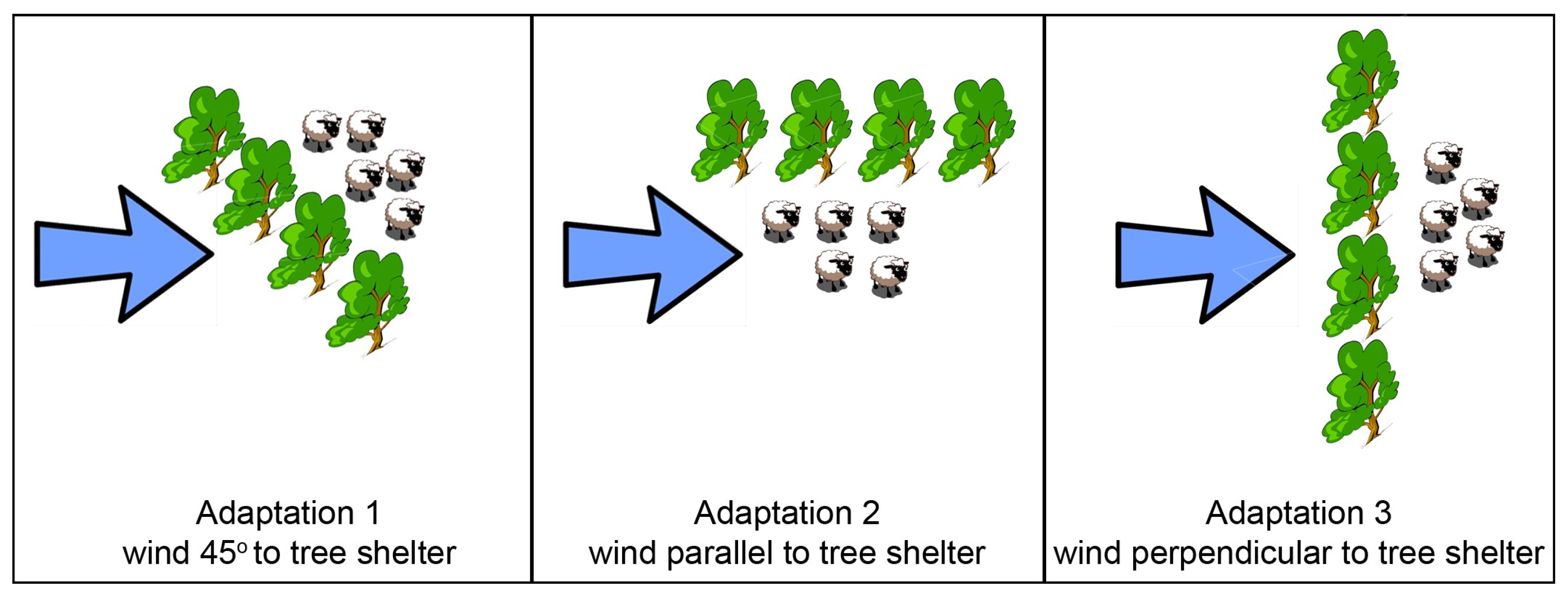
Sheep may attempt to lower heat stress by shade-seeking behaviour or restricting movements until later in the day when the temperature is lower. The modelling approach aimed at identifying the possible heat-reducing effects of a range of landscape adaptations. De Souza et al. [46] reported that the supplementation of natural or artificial shade could positively affect the feed intake and performance of lambs under warm temperature in semi-arid climates. The use of artificial shading structures may not be applicable in the Australian sheep meat industry due to the size of farms (with flock sizes regularly exceeding thousands) and the relatively low asset value of individual sheep. The use of rows of trees to provide shade appears more realistic, particularly since they are compatible with the use of farming machinery. Rows of trees of different orientation, likely having different impacts on wind speed at ground level, were considered with several possible adaptation scenarios (illustrated in Figure 7).
- No Adaptation: Where animals are submitted to “normal environmental conditions” with no alteration of wind speed or solar radiation.
- Adaptation 1: Planting of rows of trees at a 45-degree angle from the predominant wind direction, decreasing solar radiation by 65% and decreasing wind speed by 55% (extrapolated from Sudmeyer et al. [47]).
- Adaptation 2: Planting of rows of trees parallel to the predominant wind direction, decreasing solar radiation by 65% and decreasing wind speed by 25% (extrapolated from Sudmeyer et al. [47]).
- Adaptation 3: Planting of rows of trees at a 90-degree angle from the predominant wind direction, decreasing solar radiation by 65% and decreasing wind speed by 80% (extrapolated from Sudmeyer et al. [47]).
Other potential adaptations include the shearing of animals to promote thermoregulation (although this could also be counter-productive due to the possibility of cold stress in winter), improved airflow, different bedding materials to improve heat loss by conduction (although this is not practical in the field), and dietary supplements.
2.7. Specific Impact on Sheep
The thresholds used in our study to calculate HLI and AHI values were taken from the work of Gaughan et al. [2]. Sheep are more tolerant to heat stress than cows and are likely to start heating up and accumulating heat at higher thresholds than cows [8]. Conversely, sheep have a lower body weight than cows and are likely to start cooling down at higher temperatures than cows. While experimentally derived thresholds specific to sheep (not currently available) would have provided a higher level of accuracy, we believe that data based on cattle derived thresholds can still be indicative of sheep heat stress if a combination of adjusted daily maximum _ HLI, AHL, AHL_MAX, and AHI Dur values is used.
2.7.1. Estimation of Heat Stress Impact on Weight Gain
Another physiological attribute affected by heat stress is weight gain. The growth curve for lambs, representing live weight gain as a function of time, is derived from time series measurements. Models for this function have been investigated in the past, such as the Gompertz Equation, which has been investigated for sheep growth [20,21,22]. In the current study, consider weight, w, as a function of time, t, as follows:
where the transformed initial weight, G0, is given by
This is subject to:
In the previous model, one needs to find the parameters A and B. In practice, A and B have been found to be correlated and the modelling requires quite involved statistical procedures. The approach, however, provides a conceptual modelling paradigm, although implementation by numerical methods (often based on curve fitting to time series weight measurements) is usually adequate for the purpose of modelling.
Variations of exponential and power law models can also be used, whilst one convenient approach is based on regression analysis and fitting to a polynomial of appropriate order, n, as follows,
Often, a partial domain quadratic provides a sufficiently good fit over a limited range for growth curves, with or without roll-over, i.e.,
Further discussion of experimental data for regression fitting and models can be found in the published work of various researchers [19,20,21,24].
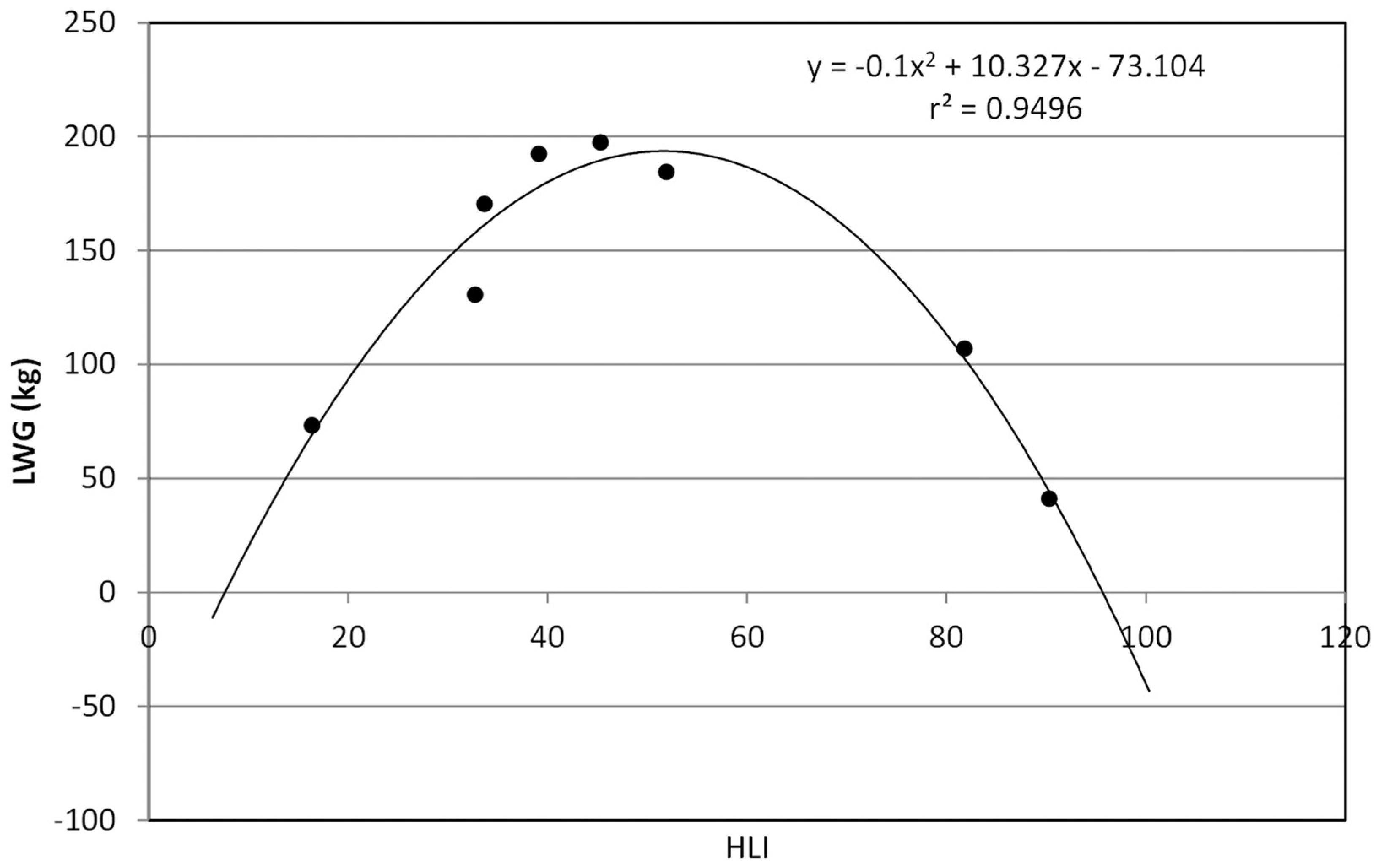
The functional dependence between HLI and lamb weight gain (LWG) is shown in Figure 8. The HLI model was fitted to the empirical data recorded by Ames and Brink (Ames and Brink, [19]). Their data collection involved careful pre-conditioning of lambs with temperature and humidity control in walk-in environmental rooms, together with an experimental duration of a 12-day treatment period. Average daily weight gain was calculated for the data (full experimental protocol can be found in the above-cited reference).
The dataset that was used in the current study using the HLI model to extrapolate for zero-weight-gain HLI effects, i.e., prediction of LWG (y) as a function of HLI (x), showed the following relationship,
The relationship allows one to derive critical information from the growth curve, i.e., for maximum weight gain:
Maximise y, i.e., solve for x,
The convex parabola representing the weight gain is a quadratic equation with roots at y = 0, i.e., utilising Equations (29) and (30); zero weight gain occurs for x-values (representing HLI), satisfying the following condition,
These estimates indicate zero weight gain at around a low level of HLI = 5 and high level of HLI = 95, with maximum weight gain at around HLI = 50. The results are indicative only and some variation may occur due to breed. Falling weight gain over HLI = 50 is due to increasing heat stress effects, such as dehydration.
While the experiment of Armes and Brink highlighted the impact of temperature (and possible HLI) on animal live weight gain, it was conducted at fixed temperatures for a period of four consecutive months [19]. It was not designed to identify the instantaneous or cumulative impact of shorter term “stress events”, and particularly heat, on daily weight gain. The results therefore could not be generalised to field conditions with varying environmental conditions or related to maximum daily HLI or AHL values. This experiment also did not explore temperatures higher than 35 degrees, where more heat stress would have occurred. Because of the lack of data that could be related to HLI or AHL, it was therefore not possible to undertake scenario analysis under different climatic conditions in addition to the analysis described.
More research is needed in the area of sheep live weight gain in relation to heat stress. Anecdotal evidence indicates that animals stressed during the day may be able to compensate by eating during the night [48,49,50]. However, no quantifications of the HLI or AHL thresholds, below which such weight gain recovery could occur, are currently available in the literature.
2.7.2. Effect of Heat Stress on Ram Fertility
In rams, there is autonomous self-regulation of scrotum temperature via the tunica dartos muscle, which pulls the testes towards the body when ambient temperature is low and away from the body when temperatures are high to dissipate excess heat (Marai et al. [50]). For spermatogenesis to proceed as normal, testis temperatures should remain at 3–4 degrees below body temperature [50]. High ambient temperature can significantly increase scrotum temperature and has been reported to be directly linked to semen damage [25,50]. Heat stress has also been reported to cause temporary interruption of sperm production and decrease libido and sperm mobility [50].
Details of biophysical responses to heat stress in sheep reproductive activity are documented in recent reviews [15,16], including effects on the libido and mounting capacity of ramss, impacts on sperm motility, and damage in spermatozoids and DNA. The testicles must remain between 2 and 8 °C below body temperature for proper functioning.
Moules and Waites [25] previously documented the effect of exposure to high temperature on the semen quality of Merino rams. In their chamber experiment, they showed semen quality could be greatly decreased (percentage of normal sperm, concentration, and live sperm) upon exposure to high temperatures (40.5 °C) for multiple hours. Their study suggested that heat stress likely damaged spermatozoa in the lumen of seminiferous tubes and potentially also affected earlier stages of spermatogenesis. It also resulted in a “latent period” lasting between approximately 10 days, for animals less sensitive to heat stress, and more than 30 days for more sensitive rams, during which sperm quality remained well below normal levels. To identify the likely occurrence of similar conditions, we identified the corresponding HLI, AHL, AHL_Max, and AHL_dur thresholds that animals were exposed to during the Moules and Waites experiment (unit conversion presented in Table 4).
Thresholds reached during the second phase of the experiment corresponded to
HLI = 101, AHL max = 90, AHL dur = 10 (hours), AHL = 0
3. Results
Our heat modelling approach was run across multiple iterations for each of the four management scenarios considered (see Table 5).
3.1. State-Wide Trend
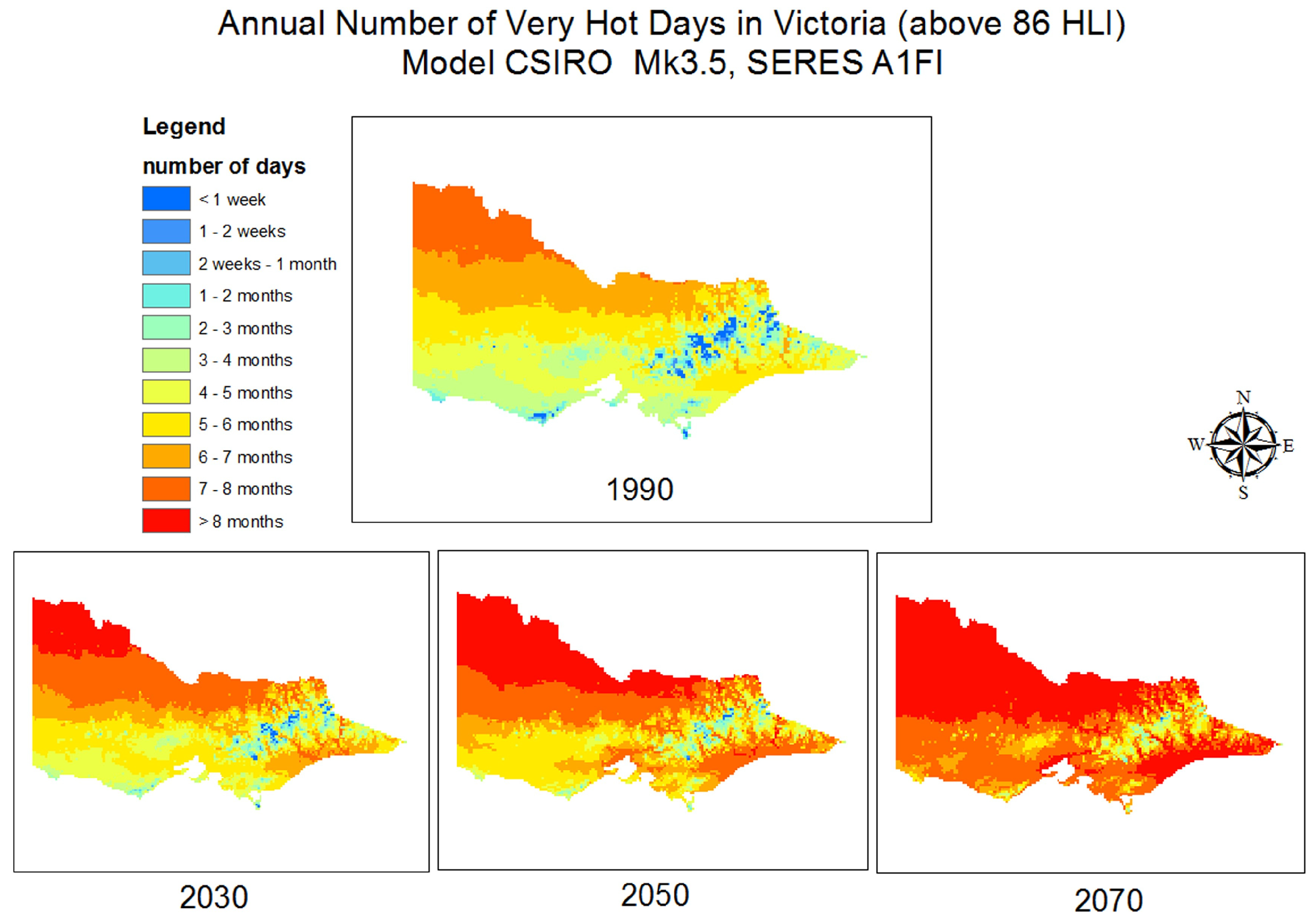
At the state level, heat stress is likely to gradually increase from the year 1990 to 2070. Figure 9, illustrating the modelled average annual cumulated number of very hot days (HLI > 86) across Victoria, clearly shows a warming trend with most of the state experiencing more than 210 very hot days per year in 2070 compared to only a few locations in 1990. Figure 10 illustrates the effects of four adaptation strategies on the number of very hot days across the state (the maximum corresponding to values modelled for the hottest location in the state while the minimum for the coolest regions). We observe that each of the adaptation scenarios considered had a general decreasing effect on the total number of very hot days across all considered years. The mitigating effect appeared highest under Scenario 2 and least under Scenario 3 across all years. However, these results only take into account one variable and the situation may be more complex when applied across the four considered variables (HLI, AHL, AHL_MAX, and AHL_dur).
3.2. Regionalisation of the Analysis
All calculations were produced across the state of Victoria at a spatial resolution of 0.05 degrees. Interpretation of these results at this level of detail is impractical so we performed a regionalisation of the results at a more relevant level. We identified six target regions based on the 2012 Victoria sheep meat and wool growing regions (Figure 1). These target regions are shown in Figure 11.
Region 1 corresponds to the Mallee region, in the furthest northwest of Victoria; Region 2 covers the Wimmera region; Region 3 covers three statistical regions, Barwon, Western District, and Central Heights, in the southwest of Victoria; Region 4 corresponds to Loddon, in central Victoria; Region 5 corresponds to the Goulburn region in central Victoria; and Region 6 corresponds to the East Gippsland area of southwest Victoria.
All results analysis were subsequently summarised for each of these six regions.
A comparison of differences for HLI, AHL, AHL_Max, and AHL_Dur across all years was undertaken using the following Z test for the hypothesis of no difference between means:
where n1 is the number of interpretations in series 1, n2 is the number of interpretations in series 2, σ is the standard deviation, and μ is the average of each series.
Results from this significance test are presented in Table 6 for the warmest region (Region 1) and the coolest region (Region 3). HLI, AHL_Max, and AHL_dur show high levels of significance, indicating that during most of the days of the year, the values taken for 1990 are significantly different from those for 2030, 2050, or 2070. This indicates that these variables are sensitive to the different years and represent suitable indicators to incorporate climate change scenario changes.
This can be explained by the fact that AHL values are null (see Figure 12) for a large proportion of the year (from June to September, corresponding to winter and early spring, when heat stress is not an issue). The conclusion from this analysis of significance is that, for the summer months (when heat stress is likely to be highest), the significant difference in climate is not lost in any of the four considered variables and they represent suitable indicators to explore implications of heat stress, despite the incorporation of the Weibull distribution inducing large levels of variation.
Results from a similar significance test across regions revealed no significant difference across HLI, AHL, AHL_Max, and AHL_Dur between Regions 2, 4, and 5, which were grouped together later on (assuming Region 4 as representative).
- Reproductive impairment due to heat stress
The impacts of heat stress on ram fertility, derived from the experimental results of Moules and Waites [25], were calculated for each selected region and each adaptation scenario. Across all regions, results for the Adaptation 1 scenario showed no noticeable differences from the “No Adaptation” scenario and are not presented here.
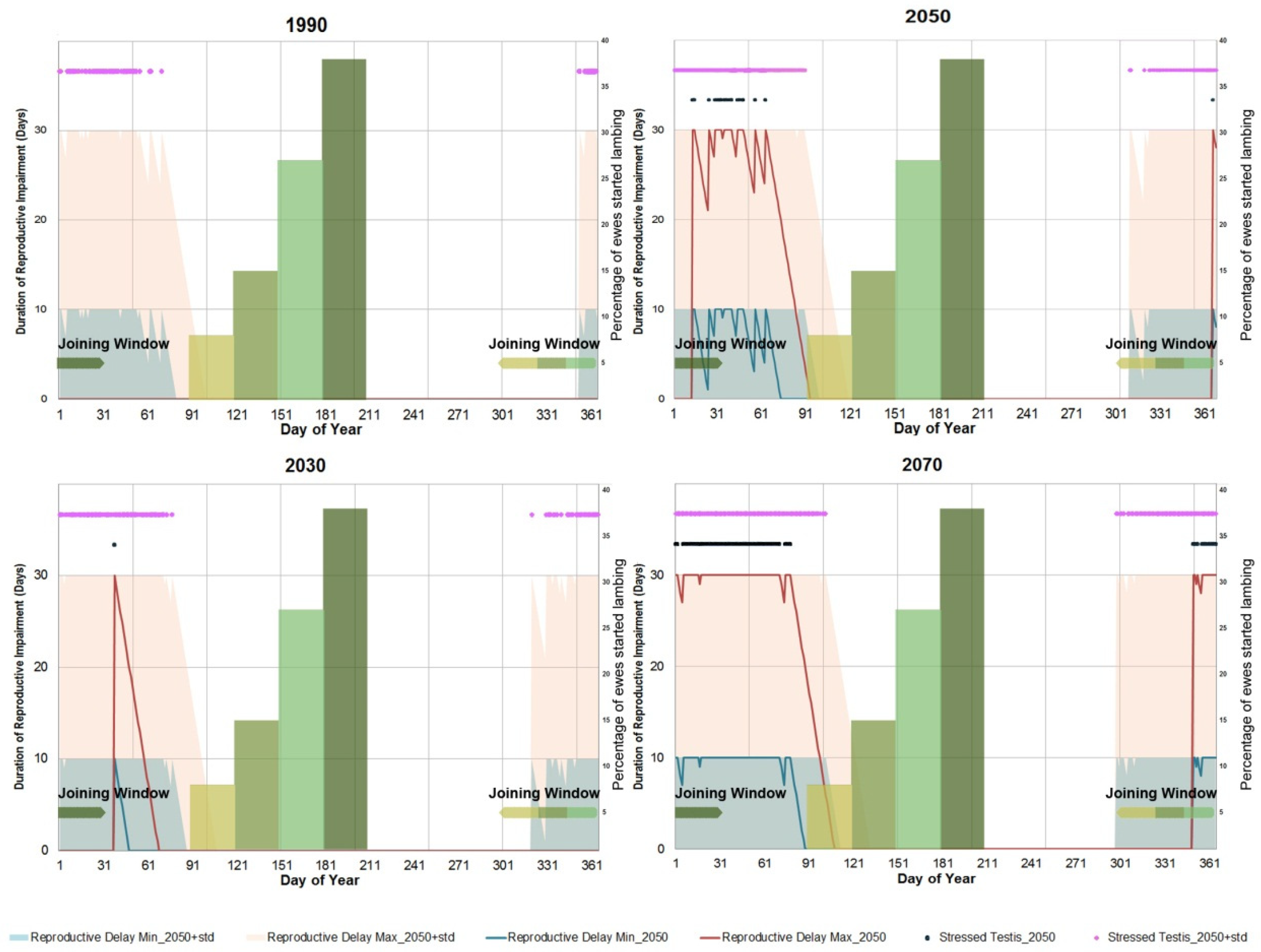
Results for Regions 1, 3, and 4 are illustrated in Figure 13, Figure 14 and Figure 15 as well as in Table 7.
Each of these figures combines, for each climate change year and day of the year, two types of information: (1) data relative to the occurrence of heat stress events and their associated periods of reproductive impairment (left Y axis); and (2) data on the current mating season and corresponding lambing period (specific to each region) (right Y axis).
Black dots in the graphs show the occurrence of stress events affecting sperm quality (identified by combinations of HLI, AHI, AHL_Max, and AHI duration) for an operating point on the risk curve of 50% (i.e., we are 50% confident conditions will be less or as stressful as indicated). These events trigger a decrease in sperm quality for a minimum period of 10 days (minimum reproductive delay), illustrated by a blue line, to a maximum 30 days (maximum reproductive delay), illustrated by a red line. Pink dots indicate the occurrence of stress events affecting sperm quality for an operating point on the risk curve of 84.1% (i.e., we are 84.1% confident that conditions will be less than or as stressful as indicated). These events trigger a decrease in sperm quality for a minimum period of 10 days, illustrated by a light blue area, to a maximum 30 days (maximum reproductive delay), illustrated by a light orange area.
The green-shaded bar chart in the centre of each graph indicates the proportion of sheep lambing for a specific region and it has a direct correlation (five months gestation) to the narrow bands of identical green shading indicating the corresponding ram/ewe joining period. For example, a joining occurring in November would lead to a delivery in April.
Figure 13, Figure 14 and Figure 15 show results for Region 1 for the No Adaptation (Figure 13), Adaptation 2 (Figure 14), and Adaptation 3 scenarios (Figure 15). Figure 13 indicates that under a No Adaptation scenario, for 1990, an overlap exists between 3/4th of the joining window and heat stress events projected from an operating point on the risk curve of 84.1%, indicating that heat stress could already be an issue for ram fertility. No overlap, however, was found for an operating point on the risk curve of 50%. From the year 2030 onwards, we observe increasing overlaps between stress events and joining windows occurring for an operating point on the risk curve of 50%. This overlap reaches 3/4 of the joining windows by 2070, indicating that in 50% of years, more than 75% of the lamb production could be threatened by heat stress.
Figure 13, Figure 14 and Figure 15 show results for Region 1 for the No Adaptation (Figure 13), Adaptation 2 (Figure 14), and Adaptation 3 scenarios (Figure 15). Figure 13 indicates that under a No Adaptation scenario, for 1990, an overlap exists between 3/4 of the joining window and heat stress events projected from an operating point on the risk curve of 84.1%, indicating that heat stress could already be an issue for ram fertility. No overlap, however, was found for an operating point on the risk curve of 50%. From the year 2030 onwards, we observe increasing overlaps between stress events and joining windows occurring for an operating point on the risk curve of 50%. This overlap reaches 3/4 of the joining windows by 2070, indicating that in 50% of years more than 75% of the lamb production could be threatened by heat stress.
Figure 14 illustrates the effects of Adaptation 2 on heat stress on rams. Across all years, this scenario appears to decrease the number of stress events for both a 50% and an 84.1% operating point on the risk curve (see Table 7), and this is particularly visible for the year 2030 where it helps avoid an overlap in the later part of the mating window (responsible for more than 35% of lambing). In 2070, it decreases chances of overlap for the early part of the mating window. These results are a clear indication of the positive impact of shade provision, via tree planting, to alleviate heat stress. However, we also observe that this adaptation does not change the overall trend of increasing overlap between stress events and mating windows and that by 2070 over 60% of lambing could be at risk in 50% of years.
Figure 15 illustrates the effect of Adaptation 3 on ram heat stress. Unlike Adaptation 2, this appears to increase the number of stress events (for both 50% and 84.1% operating points on the risk curve) (see Table 7) relatively to the No Adaptation scenario for all years. It also results in an increase in the period of time when heat stress overlaps with the joining window, particularly for 2030, 2050, and 2070 (Figure 15) when heat stress could affect more than 90% of lambing in 50% of years. These results indicate that the impact of shading structures on wind speed (which is the only difference between Adaptations 2 and 3) could very strongly affect the capacity to alleviate heat stress and could, in cases similar to Adaptation 3, make heat stress worse.
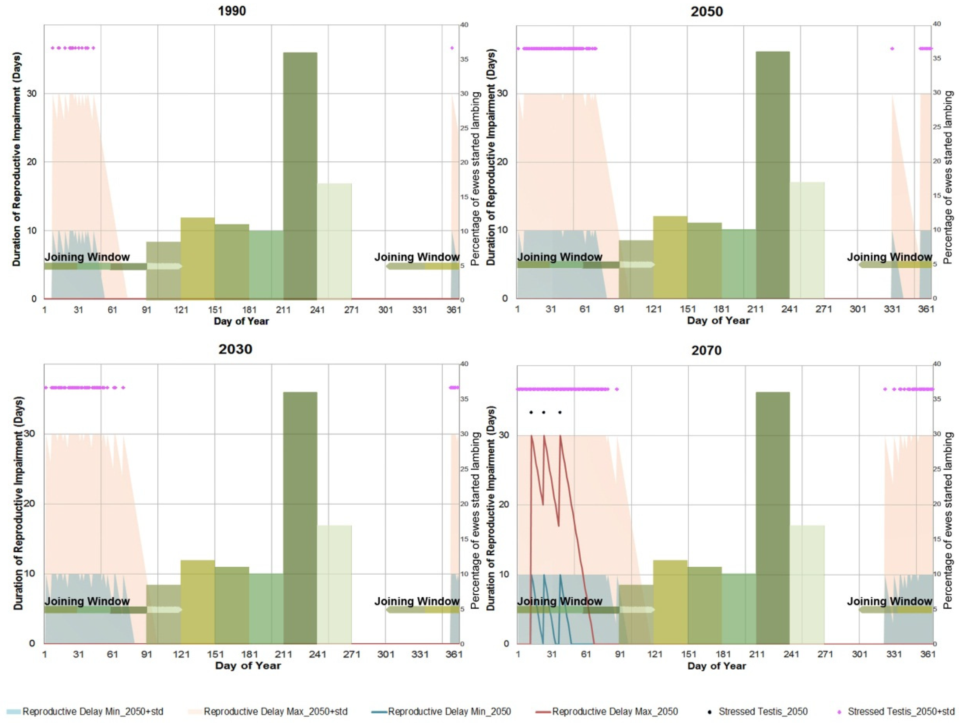
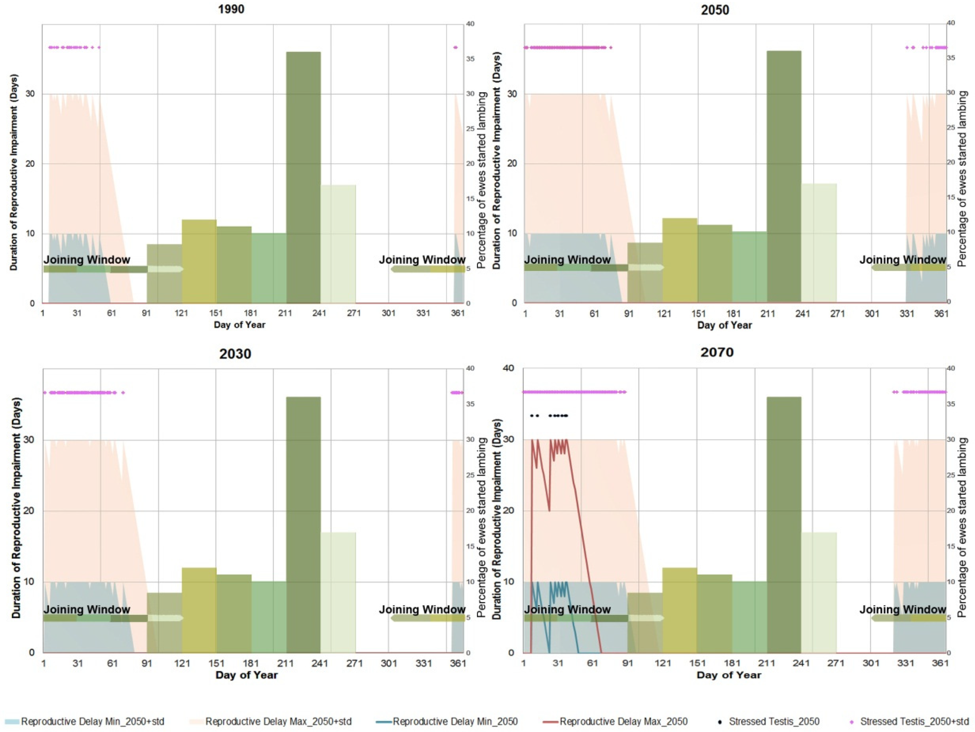
Figure 16, Figure 17 and Figure 18 show results for Region 3 for the same scenarios. This region is comparatively cooler than Region 1 and, under a No Adaptation scenario, rams exposed to these conditions appear unlikely to suffer from heat stress (for an operating point on the risk curve of 50%) from 1990 to 2050. However, by 2070, overlaps between heat stress events averaging three per year (Table 7) and the joining window could affect 20 to 30% of lambing.
Applying measures as defined by our Adaptation 2 scenario would help decrease the occurrence of heat stress events, bringing the likelihood of heat stress (for an operating point on the risk curve of 50%) to zero by 2070. The application of measures defined by Adaptation 3 would have a negative impact on heat stress, increasing the likelihood of heat stress events by 2070 whilst not significantly changing the period of time when stress and joining windows overlap (Figure 18).
Similar trends were also observed for Region 4 and Region 6 (Table 7) where heat stress is likely to become a problem from 2050 onwards for Region 4 (potentially affecting 35% of lambing in 50% of years) and 2070 onwards for Region 6. The effects of the adaptation options also appeared to be similar, with Adaptation 2 consistently leading to fewer heat stress events and Adaptation 3 leading to more heat stress events than the No Adaptation option.
4. Discussion
The occurrence of heat stress events on an hourly and daily basis were predicted using the methods described in this study. The results revealed that heat stress events, by directly affecting ram fertility, could emerge as a serious threat to the Victorian sheep industry (with stress occurring every other year) as soon as 2030 for the northern regions (i.e., Region 1) and for the whole state by 2070.
Three adaptation scenarios were investigated, based on the provision of rows of shade providing trees to alleviate heat stress. The results indicated that the effect of shading structures and wind speed, separately or together, may lead to very different outcomes. Adaptation 2, with a 20% reduction in wind speed and associated 65% reduction in solar radiation, decreased the number of heat stress events across all locations and for both 50% and 84.1% risk operating points on the risk curve. On the other hand, Adaptation 3, with an 80% reduction in wind speed and a 65% reduction in solar radiation, leads to very different outcomes. Across all regions and all years there is an increase in the predicted number of heat stress events and therefore this adaptation represents a counter-productive measure.
The provision of shade has traditionally been recommended to decrease heat stress (based on THI) in studies [52]. However, few studies have focused on the potentially negative effect of these structures on wind speed and the overall capacity of shade structures to decrease heat stress. Our results highlight the need for sheep farming enterprises to take into account the effect that rows of trees are likely to have on local wind speed before placement. Trees currently planted in paddocks for shade purposes are likely to remain in the field for several decades. If they decrease wind speed significantly, it could lead to productivity losses in the future that are higher than what they would be without shade provision.
While rows of trees planted to minimise impairment to wind can decrease the expected number of heat stress events, this adaptation will be insufficient to completely “cancel out” the impact of severe heat stress, particularly towards the second half of the century. Other adaptation options will therefore need to be considered.
A potential option would be to change the ‘timing windows’ during which the ram and ewe are brought together for mating. Moving the mating windows to earlier dates to avoid the hot season could lead to a decrease in the number of lambs being produced as sheep are physiologically adapted to breed later in the season (and rams are less fertile early in the season). Gestation occurring during the hottest months could also lead to lower reproductive rates. Moving the joining window to a later part of the year could also be problematic as the resulting lamb would be born too late in the vegetative season to benefit from maximum pasture availability and would likely require expensive fodder supplementation.
Our results based on ram fertility suggest that the effects of heat stress on sheep could have implications for the Victorian sheep industry. The impact of heat stress on other productivity components, such as animal weight gain, could also become increasingly important, and we suggest that more research is needed in the area of sheep response to heat stress.
This study highlighted gaps in the scientific literature related to heat stress on animals. Most of the published work on sheep and heat stress was based on THI and there are few experimental studies using HLI for accumulated heat stress. In most cases, solar radiation and wind information are omitted from studies, making conversion to HLI difficult.
Research is needed in the case of heat stress quantification in sheep, particularly in the identification of breed-specific thresholds. We also recommend that more experiments be conducted to identify long-to-medium-term cumulative effects of heat stress on animal appetite, daily weight gain, and embryo survival.
5. Conclusions
The study reported here applied a spatial–statistical approach to identify heat stress in grazing animals at the state-wide scale in the South-West Region of Victoria. This involved using the heat load index and accumulated heat load for heat stress assessment. Two downscaling methods were compared for application to data for temperature, humidity, solar radiation, and wind speed. Downscaling to hourly data was implemented and the modelling carried out over a 12-month cycle. Also, the HLI input of surface wind speed data appears to be the first known application in Australia using the Weibull PDF for wind speed as applied to heat stress modelling.
Various adaptations involving mitigation of solar radiation and wind to alleviate heat stress were tested, with varying success, with tree shading structures decreasing solar radiation but also limiting wind-based cooling effects.
Heat stress is also linked to ram fertility because it is a process triggered by a one-off event (physically affecting germinal cells), but data are currently lacking on long-term, cumulative effects of stress which could have an impact on animal weight gain or wool production. More research on these issues is needed to identify the possible effects of heat stress on fertility and animal growth.
The salient features of this study can be summarized as follows. The study investigated the likelihood, intensity, and duration of heat stress events in Victoria. It was demonstrated how the impact of heat stress on ram fertility could negatively affect sheep production. Shade-based mitigation strategies could have either positive or negative impacts depending on environmental variables. A key strategy needing further research and development is the impact of wind speed in combination with shade-providing structures.
Author Contributions
Conceptualization, J.-P.A. and K.K.B.; methodology, J.-P.A. and K.K.B.; formal analysis and interpretation of results, J.-P.A., K.K.B. and G.J.O.; writing, J.-P.A., K.K.B. and G.J.O.; review and editing, K.K.B. and G.J.O. All authors have read and agreed to the published version of the manuscript.
Funding
This research was supported by the Department of Environment and Primary Industries Risk Analysis for Resilient Agriculture Project CMI 103757.
Data Availability Statement
Meteorological data is publicly available (see text). Data supporting the findings of this study will be available on reasonable request from the corresponding author.
Acknowledgments
The authors thank present and former colleagues for valuable insights and data for analysis. In particular, we thank Falak Sheth and Anna Weeks. Also, Ralph Behrendt, Malcolm McCaskill, Matthew Knight, Fiona Cameron, John Byron, Andrew Kennedy, Steve Clark, and Ellen Jongman for providing advice on sheep physiology.
Conflicts of Interest
The authors declare no conflicts of interest.
References
- Silanikove, N. Effects of heat stress on the welfare of extensively managed domestic ruminants. Livest. Prod. Sci. 2000, 67, 1–18. [Google Scholar] [CrossRef]
- Gaughan, J.B.; Mader, T.L.; Holt, S.M.; Lisle, A. A new heat load index for feedlot cattle. J. Anim. Sci. 2008, 86, 226–234. [Google Scholar] [CrossRef]
- Little, S.; Campbell, J. Cool Cows: Dealing with Heat Stress in Australian Dairy Herds Dairy Australia; Dairy Australia: Melbourne, VIC, Australia, 2008. [Google Scholar]
- Smith, D.M.S.; Noble, I.R.; Jones, G.K. A heat balance model for sheep and its use to predict shade-Seeking behaviour in hot conditions. J. Appl. Ecol. 1985, 22, 753–774. [Google Scholar] [CrossRef]
- Benke, K.K.; Benke, L.R. Experiments in Optimal Spatial Segmentation of Local Regions Using Categorical and Quantitative Data. Appl. Spat. Anal. Policy 2013, 6, 185–208. [Google Scholar] [CrossRef]
- Finch, V.A. Body Temperature in Beef Cattle: Its Control and Relevance to Production in the Tropics. J. Anim. Sci. 1986, 62, 531–542. [Google Scholar] [CrossRef]
- Beede, D.K.; Collier, R.J. Potential Nutritional Strategies for Intensively Managed Cattle during Heat Stress. J. Anim. Sci. 1986, 62, 543–550. [Google Scholar] [CrossRef]
- Mayer, D.G.; Davison, T.M.; McGowan, M.R.; Young, B.A.; Matschoss, A.L.; Hall, A.B.; Goodwin, P.J.; Jonsson, N.N.; Gaughan, J.B. Extent and economic effect of heat loads on dairy cattle production in Australia. Aust. Vet. J. 1999, 77, 804–808. [Google Scholar] [CrossRef] [PubMed]
- Jones, R.N.; Hennessy, K.J. Climate Change Impacts in the Hunter Valley: A Risk Assessment of Heat Stress Affecting Dairy Cattle; CSIRO Division of Atmospheric Research: Aspendale, VIC, Australia, 2000. [Google Scholar]
- Mader, T.; Davis, S.; Gaughan, J.; Brown-Brandl, T. Wind Speed and Solar Radiation Adjustments for the Temperature-Humidity Index. In Proceedings of the 16th Conference on Biometeorology and Aerobiology, Vancouver, BC, Canada, 23–27 August 2004; pp. 57–62. [Google Scholar]
- Berman, A.; Folman, Y.; Kaim, M.; Mamen, M.; Herz, Z.; Wolfenson, D.; Arieli, A.; Graber, Y. Upper Critical Temperatures and Forced Ventilation effects for high-yielding Dairy Cows in a Sub-tropical Climate. J. Dairy Sci. 1985, 68, 488–495. [Google Scholar] [CrossRef] [PubMed]
- Eigenberg, R.A.; Brown-Brandl, T.M.; Nienaber, J.A.; Hahn, G.L. Dynamic response indicators of heat stress in shaded and non-shaded feedlot cattle, part 2: Predictive relationships. Biosyst. Eng. 2005, 91, 111–118. [Google Scholar] [CrossRef]
- Gaughan, J.B. Respiration rate—Is it a good measure of heat stress in cattle? Asian-Australas. J. Anim. Sci. 2000, 13, 329–332. [Google Scholar]
- Gaughan, J.B.; Lees, J.C. Categorising heat load on dairy cows. In Proceedings of the 28th Biennial Conference of the Australian Society of Animal Production, Armidale, NSW, Australia, 11–15 July 2010. [Google Scholar]
- Sierra, A.B.; Avendaño, R.L.; Hernández, R.J.A.; Pérez, R.V.; Calderón, A.C.; Mellado, M.; Cesar, A.; Herrera, M.; Cruz, U.M. Thermoregulation and reproductive responses of rams under heat stress. Review. Rev. Mex. Cienc. Pec. 2021, 12, 910–931. [Google Scholar]
- van Wettere, W.H.; Kind, K.L.; Gatford, K.L.; Swinbourne, A.M.; Leu, S.T.; Hayman, P.T.; Kelly, J.M.; Weaver, A.C.; Kleemann, D.O.; Walker, S.K. Review of the impact of heat stress on reproductive performance of sheep. J. Anim. Sci. Biotechnol. 2021, 12, 26. [Google Scholar] [CrossRef] [PubMed]
- Stockman, C.A. The Physiological and Behavioural Responses of Sheep Exposed to Heat Load within Intensive Sheep Industries, School of Biomedical and Veterinary Sciences; Murdoch University: Murdoch, WA, USA, 2006. [Google Scholar]
- Pelizaro, C.; Benke, K.; Sposito, V. A modelling framework for optimisation of commodity production by minimising the impact of climate change. Appl. Spat. Anal. Policy 2011, 4, 201–222. [Google Scholar] [CrossRef]
- Ames, D.R.; Brinks, D.R. Effect of temperature on lamb performance and protein efficiency ratio. J. Anim. Sci. 1977, 44, 136–144. [Google Scholar] [CrossRef]
- Lewis, R.M.; Brotherstone, S. A genetic evaluation of growth in sheep using random regression techniques. Anim. Sci. 2002, 74, 63–70. [Google Scholar] [CrossRef]
- Lewis, R.M.; Emmans, G.C.; Dingwall, W.S.; Simm, G. A description of the growth of sheep and its genetic analysis. Anim. Sci. 2002, 74, 51–62. [Google Scholar] [CrossRef]
- Bardos, D.C. Probabilistic Gompertz model of irreversible growth. Bull. Math. Biol. 2005, 67, 529–545. [Google Scholar] [CrossRef]
- Freund, J.E. Mathematical Statistics; Prentice Hall: Upper Saddle River, NJ, USA, 1972. [Google Scholar]
- Lambe, N.R.; Navajas, E.A.; Simm, G.; Bünger, L. A genetic investigation of various growth models to describe growth of lambs of two contrasting breeds. J. Anim. Sci. 2006, 84, 2642–2654. [Google Scholar] [CrossRef]
- Moule, G.R.; Waites, G.M. Seminal degeneration in the ram and its relation to the temperature of the scrotum. J. Reprod. Fertil. 1963, 5, 433–446. [Google Scholar] [CrossRef]
- Marai, I.F.M.; El-Darawany, A.A.; Fadiel, A.; Abdel-Hafez, M.A.M. Physiological traits as affected by heat stress in sheep—A review. Small Rumin. Res. 2007, 71, 1–12. [Google Scholar] [CrossRef]
- Papanastasiou, D.K. Classification of potential sheep heat-stress levels according to the prevailing meteorological conditions. Agric. Eng. Int. CIGR J. 2015, 57–64. [Google Scholar]
- Sejian, V.; Bhatta, R.; Gaughan, J.B.; Dunshea, F.R.; Lacetera, N. Adaptation of animals to heat stress. Animal 2018, 12, s431–s444. [Google Scholar] [CrossRef] [PubMed]
- Berihulay, H.; Abied, A.; He, X.; Jiang, L.; Ma, Y. Adaptation mechanisms of small ruminants to environmental heat stress. Animals 2019, 9, 75. [Google Scholar] [CrossRef] [PubMed]
- Lees, A.M.; Sullivan, M.L.; Olm JC, W.; Cawdell-Smith, A.J.; Gaughan, J.B. The influence of heat load on Merino sheep. 1. Growth, performance, behaviour and climate. Anim. Prod. Sci. 2020, 60, 1925–1931. [Google Scholar] [CrossRef]
- Tadesse, D.; Patra, A.K.; Puchala, R.; Goetsch, A.L. Effects of High Heat Load Conditions on Blood Constituent Concentrations in Dorper, Katahdin, and St. Croix Sheep from Different Regions of the USA. Animals 2022, 12, 2273. [Google Scholar] [CrossRef] [PubMed]
- Lees, A.M.; Sullivan, M.L.; Cawdell-Smith, A.J.; Gaughan, J.B. 505 Developing heat stress thresholds for sheep. J. Anim. Sci. 2017, 95 (Suppl. 4), 246–247. [Google Scholar] [CrossRef]
- McCarthy, M.; Fitzmaurice, L. Heat Load Forecasting Review; Final Report B.FLT.0393; Meat and Livestock Australia Ltd.: North Sydney, NSW, Australia, 2016. [Google Scholar]
- Wilby, R.L.; Wigley, T.M. Downscaling general circulation model output: A review of methods and limitations. Prog. Phys. Geogr. 1997, 21, 530–548. [Google Scholar] [CrossRef]
- Darbyshire, R.; Webb, L.; Goodwin, I.; Barlow, S. Winter chilling trends for deciduous fruit trees in Australia. Agric. For. Meteorol. 2011, 151, 1074–1085. [Google Scholar] [CrossRef]
- Chow, D.H.C.; Levermore, G.J. New algorithm for generating hourly temperature values using daily maximum, minimum and average values from climate models. Build. Serv. Eng. Res. Technol. 2007, 28, 237–248. [Google Scholar] [CrossRef]
- Weeks, A.; Christy, B.; O’Leary, G. Generating daily future climate scenarios for crop simulation. In Proceedings of the 15th Australian Agronomy Conference, Lincoln, New Zealand, 15–18 November 2010. [Google Scholar]
- Monahan, A.H.; He, Y.; McFarlane, N.; Dai, A. The probability distribution of land surface wind speeds. J. Clim. 2011, 24, 3892–3909. [Google Scholar] [CrossRef]
- Pryor, S.C.; Schoof, J.T.; Barthelmie, R.J. Empirical downscaling of wind speed probabilty distributions. J. Geophys. Res. D Atmos. 2005, 110, 1–12. [Google Scholar] [CrossRef]
- Weibull, W. A statistical distribution function of wide applicability. J. Appl. Mech. 1951, 18, 292–297. [Google Scholar] [CrossRef]
- CSIRO. OzClim—Exploring Climate Change Scenarios for Australia; CSIRO: Canberra, ACT, Australia, 2010. [Google Scholar]
- BOM. Rainfall Percentages; Australian Bureau of Meteorology: Commonwealth of Australia, Melbourne, Australia, 2013. [Google Scholar]
- Jeffrey, S.J.; Carter, J.O.; Moodie, K.B.; Beswick, A.R. Using spatial interpolation to construct a comprehensive archive of Australian climate data. Environ. Model. Softw. 2001, 16, 309–330. [Google Scholar] [CrossRef]
- IPCC. Climate Change 2007: Synthesis Report, Contribution of Working Groups I, II and III to the Fourth Assessment Report of the Intergovernmental Panel on Climate Change; IPCC: Geneva, Switzerland, 2007. [Google Scholar]
- IPCC. Summary for Policymakers; Solomon, S., Qin, D., Manning, M., Chen, Z., Marquis, M., Averyt, K.B., Eds.; IPCC: Geneva, Switzerland, 2007. [Google Scholar]
- de Souza, B.B.; Andrade, I.S.; Filho, J.M.P.; Silva, A.M.A. Environmental and supplementation effect on the alimentary behavior and on performance of lambs in semiarid. Caatinga 2011, 24, 123–129. [Google Scholar]
- Sudmeyer, R.; Bicknell, D.; Coles, N. Tree Windbreaks in the Wheatbelt; Bulletin 4723; Department of Primary Industries and Regional Development: Perth, WA, Australia, 2007; p. 27. [Google Scholar]
- Metzger, M. Avoid Heat Stress in Your Sheep and Goats; Michigan State University: East Lansing, MI, USA, 2012. [Google Scholar]
- Jongman, E. Personal Communication on sheep heat stress, 2013.
- Marai, I.F.M.; El-Darawany, A.H.A.; Ismail, E.S.A.F.; Abdel-Hafez, M.A.M. Tunica dartos index as a parameter for measurement of adaptability of rams to subtropical conditions of Egypt. Anim. Sci. J. 2006, 77, 487–494. [Google Scholar] [CrossRef]
- Brice, T.; Hall, T. Vapor Pressure; National Weather Service Weather Forecast, US Department of Commerce: Santa Teresa, NM, USA, 2013. [Google Scholar]
- Morrison, S.R. Ruminant heat stress: Effect on production and means of alleviation. J. Anim. Sci. 1983, 57, 1594–1600. [Google Scholar] [CrossRef]
Figure 1.
External stressors associated with heat stress in sheep.

Figure 2.
Example of model vs. measured data for solar radiation for a 24 h period in Hamilton, Victoria.
Figure 2.
Example of model vs. measured data for solar radiation for a 24 h period in Hamilton, Victoria.

Figure 3.
Weibull probability distribution for wind speed and histogram data.

Figure 4.
Comparison of measured versus model relative humidity on a rainy day at Hamilton in regional Victoria.
Figure 4.
Comparison of measured versus model relative humidity on a rainy day at Hamilton in regional Victoria.

Figure 5.
A sampling rate of every fourth value was used for the time series of the wind probability distribution to lower the incidence of correlation.
Figure 5.
A sampling rate of every fourth value was used for the time series of the wind probability distribution to lower the incidence of correlation.

Figure 6.
The Q–Q plot for the wind speed data distribution vs. Weibull distribution.

Figure 7.
Illustration of adaptation options investigated, relative to main wind direction.

Figure 8.
Example of functional dependence of lamb weight gain (LWG) vs. heat load index (HLI). The model is fitted to published data [19].
Figure 8.
Example of functional dependence of lamb weight gain (LWG) vs. heat load index (HLI). The model is fitted to published data [19].

Figure 9.
Estimated changes in the number of very hot days (HLI > 86) across the state of Victoria for 1990, 2030, 2050, and 2070.
Figure 9.
Estimated changes in the number of very hot days (HLI > 86) across the state of Victoria for 1990, 2030, 2050, and 2070.

Figure 10.
Distribution of the projected number of very hot days (HLI > 86) across Victoria for 1990, 2030, 2050, and 2070 under four adaptation scenarios.
Figure 10.
Distribution of the projected number of very hot days (HLI > 86) across Victoria for 1990, 2030, 2050, and 2070 under four adaptation scenarios.

Figure 11.
Regions of interest selected for investigation. Digitized from the 2012 Victoria sheep meat and wool growing regions (https://vgls.sdp.sirsidynix.net.au/client/search/asset/1299288/0, accessed 15 January 2024), representing Mesh Block boundaries as defined by the Australian Statistical Geography Standard (ASGS) where more than 20,000 sheep and lambs were present. The regions were selected because of the interest of local farmers.

Figure 12.
AHL for Region 1 comparing outputs from the years 2050 and 2070 under a do-nothing scenario.
Figure 12.
AHL for Region 1 comparing outputs from the years 2050 and 2070 under a do-nothing scenario.

Figure 13.
Occurrence and duration of reproductive impairment associated with heat stress for Region 1 under a No Adaptation scenario for the years 1990, 2030, 2050, and 2070.
Figure 13.
Occurrence and duration of reproductive impairment associated with heat stress for Region 1 under a No Adaptation scenario for the years 1990, 2030, 2050, and 2070.

Figure 14.
Occurrence and duration of reproductive impairment associated with heat stress in Region 1 under an Adaptation 2 scenario for the years 1990, 2030, 2050, and 2070.
Figure 14.
Occurrence and duration of reproductive impairment associated with heat stress in Region 1 under an Adaptation 2 scenario for the years 1990, 2030, 2050, and 2070.

Figure 15.
Occurrence and duration of reproductive impairment associated with heat stress in Region 1 under an Adaptation 3 scenario for the years 1990, 2030, 2050, and 2070.
Figure 15.
Occurrence and duration of reproductive impairment associated with heat stress in Region 1 under an Adaptation 3 scenario for the years 1990, 2030, 2050, and 2070.

Figure 16.
Occurrence and duration of reproductive impairment associated with heat stress in Region 3 under a No Adaptation scenario for the years 1990, 2030, 2050, and 2070.
Figure 16.
Occurrence and duration of reproductive impairment associated with heat stress in Region 3 under a No Adaptation scenario for the years 1990, 2030, 2050, and 2070.

Figure 17.
Occurrence and duration of reproductive impairment associated with heat stress in Region 3 under an Adaptation 2 scenario for the years 1990, 2030, 2050, and 2070.
Figure 17.
Occurrence and duration of reproductive impairment associated with heat stress in Region 3 under an Adaptation 2 scenario for the years 1990, 2030, 2050, and 2070.

Figure 18.
Occurrence and duration of reproductive impairment associated with heat stress in Region 3 under an Adaptation 3 scenario for the years 1990, 2030, 2050, and 2070.
Figure 18.
Occurrence and duration of reproductive impairment associated with heat stress in Region 3 under an Adaptation 3 scenario for the years 1990, 2030, 2050, and 2070.


Table 1.
Comparison between Darbyshire and CBSE methods.
| Site | Darbyshire RMSE in °C | CBSE Linking Days RMSE in °C |
|---|---|---|
| Hamilton | 2.6 | 2.2 |
| Tatura * | 5.5 | 5.1 |
* with 1397 missing data points.
Table 2.
The R2 values for comparison of measured versus modelled data.
| Variable | R2 |
|---|---|
| Temperature | 0.894 |
| Relative humidity | 0.7005 |
| Solar radiation | 0.8545 |
| Wind | 0.9774 (ordered) |
Table 3.
Variables used in the model *.
| Variable | Description | Unit |
|---|---|---|
| Tmin | Minimum daily temperature | °C |
| Tmax | Maximum daily temperature | °C |
| RHmin | Minimum relative humidity | % |
| RHmax | Maximum relative humidity | % |
| Rad | Daily solar radiation | MJ/m2/Day |
* Data sourced from Hamilton (Station #90173, Lat. −37.65, Long. 142.06) and Tatura (Station #81049, Lat. −36.44, Long. 145.27) locations managed by the Australian Bureau of Meteorology.
Table 4.
HLI model variables.
| Variable | Values |
|---|---|
| Temperature | 40.5 °C |
| Relative humidity | 55.64%: derived from 31.5 mmHG assuming a saturated vapour pressure at 40.5 degrees = 75.49; see [51]. |
| Solar radiation | 1.61 Wm−2: derived from recommended light conditions in environmental rooms, range of 1100 Lux [52], corresponding to approximately 1.6 Wm−2 |
| Wind speed | 0.3 ms−1 |
Table 5.
Management scenarios.
| Landscape Option | Number of Model Iterations |
|---|---|
| Do nothing | 157 |
| Adaptation 1 | 133 |
| Adaptation 2 | 112 |
| Adaptation 3 | 109 |
Table 6.
Number of days where statistically significant difference was observed (Threshold 5) (HLI = heat load index, AHL = accumulated heat load, with AHL maximum and duration).
Table 6.
Number of days where statistically significant difference was observed (Threshold 5) (HLI = heat load index, AHL = accumulated heat load, with AHL maximum and duration).
| Comparison 1990–2030 | Comparison 2030–2050 | Comparison 2030–2070 | ||||
|---|---|---|---|---|---|---|
| Variable | Region 1 | Region 3 | Region 1 | Region 3 | Region 1 | Region 3 |
| HLI | 303 | 324 | 364 | 147 | 364 | 364 |
| AHL | 171 | 109 | 161 | 68 | 248 | 175 |
| AHL_Max | 340 | 104 | 347 | 86 | 365 | 319 |
| AHL Dur | 359 | 277 | 363 | 364 | 345 | 56 |
Table 7.
Number of heat stress events showing the advantage of less heat stress events in Adaptation 2.
Table 7.
Number of heat stress events showing the advantage of less heat stress events in Adaptation 2.
| Number of Heat Stress Events | ||||||||||||
|---|---|---|---|---|---|---|---|---|---|---|---|---|
| Region 1 | Region 3 | Region 4 | Region 6 | |||||||||
| Year | No Adaptation | Adaptation 2 | Adaptation 3 | No Adaptation | Adaptation 2 | Adaptation 3 | No Adaptation | Adaptation 2 | Adaptation 3 | No Adaptation | Adaptation 2 | Adaptation 3 |
| 1990 | 0 | 0 | 0 | 0 | 0 | 0 | 0 | 0 | 0 | 0 | 0 | 0 |
| 2030 | 4 | 1 | 15 | 0 | 0 | 0 | 0 | 0 | 1 | 0 | 0 | 0 |
| 2050 | 34 | 22 | 66 | 0 | 0 | 0 | 7 | 2 | 25 | 0 | 0 | 2 |
| 2070 | 93 | 84 | 118 | 3 | 0 | 8 | 72 | 62 | 84 | 11 | 5 | 28 |
| 1990+Std Dev | 76 | 59 | 85 | 15 | 6 | 26 | 49 | 35 | 66 | 13 | 8 | 17 |
| 2030+Std Dev | 117 | 102 | 127 | 49 | 33 | 61 | 89 | 81 | 106 | 49 | 28 | 65 |
| 2050+Std Dev | 137 | 136 | 146 | 71 | 64 | 85 | 121 | 113 | 131 | 80 | 67 | 95 |
| 2070+Std Dev | 171 | 165 | 178 | 106 | 93 | 121 | 147 | 143 | 162 | 121 | 114 | 130 |
Disclaimer/Publisher’s Note: The statements, opinions and data contained in all publications are solely those of the individual author(s) and contributor(s) and not of MDPI and/or the editor(s). MDPI and/or the editor(s) disclaim responsibility for any injury to people or property resulting from any ideas, methods, instructions or products referred to in the content. |
© 2024 by the authors. Licensee MDPI, Basel, Switzerland. This article is an open access article distributed under the terms and conditions of the Creative Commons Attribution (CC BY) license (https://creativecommons.org/licenses/by/4.0/).
Share and Cite
MDPI and ACS Style
Aurambout, J.-P.; Benke, K.K.; O’Leary, G.J. Accumulative Heat Stress in Ruminants at the Regional Scale under Changing Environmental Conditions. Environments 2024, 11, 55. https://doi.org/10.3390/environments11030055
AMA Style
Aurambout J-P, Benke KK, O’Leary GJ. Accumulative Heat Stress in Ruminants at the Regional Scale under Changing Environmental Conditions. Environments. 2024; 11(3):55. https://doi.org/10.3390/environments11030055
Chicago/Turabian StyleAurambout, Jean-Philippe, Kurt K. Benke, and Garry J. O’Leary. 2024. "Accumulative Heat Stress in Ruminants at the Regional Scale under Changing Environmental Conditions" Environments 11, no. 3: 55. https://doi.org/10.3390/environments11030055
Note that from the first issue of 2016, this journal uses article numbers instead of page numbers. See further details here.