
Acoustic Characterization of Potential Quiet Areas in Dortmund, Germany

1
Research Group Landscape Ecology and Landscape Planning, Department of Spatial Planning, TU Dortmund University, 44221 Dortmund, Germany
2
Department of Climate Protection, Climate Impact Adaptation, and Immission Control, Environmental Office, 44135 Dortmund, Germany
*
Author to whom correspondence should be addressed.
Environments 2024, 11(4), 69; https://doi.org/10.3390/environments11040069
Submission received: 22 February 2024
/
Revised: 19 March 2024
/
Accepted: 25 March 2024
/
Published: 31 March 2024
(This article belongs to the Special Issue New Solutions Mitigating Environmental Noise Pollution II)
Abstract
:German noise action plans aim to reduce negative health outcomes from noise exposure and identify quiet areas free of noise pollution. Quiet area identification in German noise action plans is based primarily on noise mapping and spatial analysis and not empirical or qualitative data about acoustic environments, thus leaving a gap in the understanding of the quality of formally recognized quiet areas in noise action plans. This work presents a comparative empirical case study in Dortmund, Germany, with the aim to describe the diurnal dB(A) and biophonic properties of quiet areas versus noise ‘hot spots’. Sound observations (n = 282,764) were collected in five different natural or recreational land use patch types larger than four acres within 33 proposed quiet areas in Dortmund (n = 70) and 23 noise hot spots between 27 April 2022 and 2 March 2023. We found that quiet areas are on average more than 20 dB(A) quieter than noise hot spots almost every hour of the day. Forests, managed tree stands, cemeteries, and agriculture diel patterns are dominated by dawn dusk chorus in spring and summer, whereas sports and recreation as well as noise hot spots are dominated by traffic and human noise. A novel composite biophony mapping procedure is presented that finds distinct temporal distribution of biophony in forested and agriculture peri-urban locations positively associated with patch size, distance away from LDEN > 55, proximity to water, and the number of vegetation layers in the plant community. Anthrophony distribution dominates urban land uses in all hours of the day but expands during the day and evening and contracts at night and in dusk hours. The procedures presented here illustrate how qualitative information regarding quiet areas can be integrated into German noise action planning.
1. Introduction
The current practice of noise management in Germany includes the use of noise mapping to identify locations where legally defined thresholds for calculated noise levels during certain hours of the day are exceeded (§47c, 47d, 47f German Federal Immission Control Act (BImSchG); 34. German Federal Immission Control Ordinance (BImSchV)). This planning instrument focuses on road, rail, airplane, and industry source emissions to map averaged and weighted decibel levels (LDEN). Noise thresholds are based on research indicating that continuous noise exposure is a human health risk that leads to annoyance and stress [1], hypertension [2], heart attack [3], stroke [4], atherosclerosis [5], or depression [6,7]. However, since noise propagation models are based solely on sound pressure level (SPL) measures, the resultant noise maps leave little information about the acoustic environment when SPLs are below legally defined noise thresholds. In this case, areas below noise thresholds simply appear as blank spots on noise maps. Noise hot spots where the highest LDEN levels are reached are often the main focus of noise action plan recommendations, especially since reducing exposure is one of the main aims of noise action planning (§47 BImSchG). However, an array of information about acoustic environments beyond SPL measures has emerged in the overlapping fields of ecoacoustics [8], soundscape ecology [9], and soundscape studies [10], from which a set of ecoacoustic indices has emerged [11,12] to study the acoustic environment beyond the noise paradigm.
Guidance on the identification of so called ‘quiet areas’ from the European Environmental Agency (EEA) indicates that absolute silence is not the goal of quiet areas but rather they aim to identify calm, tranquil, or relaxing acoustic environments [13]. The EEA indicates that only marginal evidence exists to claim that quiet areas are good for human health. However, the known health benefits include reduced annoyance at LAeq < 45 dB, proximity to green areas in general [14,15], and increased recovery in patients in quiet acoustic environments [16] away from major transport lines or industry in rural areas [13] that contain natural sounds [17,18]. For the time being, the EEA recommends that quiet area identification should be focused on acoustic environments that provide rest, relaxation, peace of mind, or calm in the vicinity of their homes or in accessible peri-urban locations that contain natural sounds [13].
The aim of this study is to introduce an empirical approach to characterize the spatial and temporal variation in SPLs and the biophonic quality of potential quiet areas, which conforms to the requirements of the EU noise directive, can be carried out at the city-wide scale independent of participants required for the soundscape protocol, and acts as a counterpoint to noise mapping within the German noise action plan. The City of Dortmund, currently updating its noise action plan, serves as a ‘living lab’ and the methods and outputs are examples of how scientific advising via the noise advisory board can inform legal designation of quiet areas according to [19].
1.1. Natural Sounds and Quiet Area Identification
To identify quiet areas, the EEA recommends the use of a set of selection criteria, including dB-based indicators such as LEQ 24h, LDEN, LN, or LDAY; psychoacoustic indicators that have perceived acoustic quality/appreciation based on the Soundscape approach [20]; functional indicators such as restoration or nature protection areas with ‘restorative’ functions or established positive visual attributes in formal landscape or nature conservation plans; and spatial indicators such as locations placed 4–15 km away from motorways and 1–4 km away from urban agglomerations, with sizes ranging in area from 1 to 4 km2 for rural locations and 100 m2 to 0.1 km2 in urban areas [13] (p. 10). The indicators above are to be supported with spatial overlay modelling where roadway distance thresholds, the degree of natural and rural land cover based on the Corine Land Cover dataset, and population density are reclassified as a suitability index for quietness [13] (pp. 41–50). While this approach may identify areas without road or rail noise, it does not include any method of determination regarding the source of sounds within the spatially identified quiet areas. Considering that the EU’s guidance is not the identification of absolute silence, the development of a biophonic mapping method to verify, rank, or optimize quiet area selection is a relevant current research gap in the EU Noise Directive [21].
1.2. Quiet Areas in German Noise Action Plans
Refocusing the discussion on quiet area planning within the German noise action plan (BImSchG, §§47a–f), we find that national-level examples of quiet area selection in Munich, Berlin, and Braunschweig do not include perception-based factors in the identification of quiet areas; rather, they rely on the spatial buffer and nature protection area approaches to identify quiet areas [22]. This reality is likely due to the difficulty cities face in carrying out time and human participant intensive soundwalk studies at the city-wide or regional scale.
In the Ruhr urban agglomeration, we review quiet area selection methods within the most recent noise action plans in the four largest cites of Dortmund [23], Bochum [24], Essen [25], and Duisburg [26], finding that all cities have noise action plans with quiet area designations but do not use any factors of perceived soundscape quality or empirical measures of frequency ranges in the weighting and selection process. The city of Dortmund noise action plan 2014 [23] utilizes the LDEN < 55 dB(A) threshold to identify areas of 50–100+ ha with known restorative functions based on nature protection status, as elaborated in the formal landscape plan instrument. The quiet area criteria in Bochum includes peri-urban nature and landscape protection areas over 4 km2 with LDEN < 50 dB(A), inner-city parks, green spaces, small garden areas, pure residential areas with interior zones 6 dB(A) quieter than the residential area edges, and linear green corridors of at least 1000 m [24]. The city of Essen includes areas of LDEN < 50 dB(A) in peri-urban land uses of parks, forests, surface water, and agriculture with a minimum area of 100 ha, and inner-city green spaces over 3 ha with LDEN < 55 dB(A) with a restorative function per the landscape plan instrument near residential developments [25]. The city of Duisburg identifies peri-urban quiet areas in forest, agricultural, or water areas over 4 km2 where LDEN ≤ 55 dB(A) included in the landscape plan (BNatSchG §11). However, in Duisburg, there are no inner-city areas below LDEN 55 according to the noise map (BImSchG §47c) and thus green spaces near to residential areas that are 6 dB(A) quieter than surrounding LDEN values are selected as inner-city quiet areas [26].
Thus, the identification of quiet areas within noise action plans in Germany is developing based on spatial modelling without soundscape perception or sound source data with relatively new guidance from the German Environment Agency [22]. The resultant quiet areas themselves are not stratified in any way, leading to the conclusion that the acoustic environment, outside of the LDEN values, is homogeneous. However, anybody who has stood in a large wind-swept peri-urban agricultural field versus deep in a tall mixed temperate deciduous forest knows that while both areas may be quiet, the quality of ‘natural sounds’, such as birds or rustling leaves, creates different acoustic environments. If the aim of quiet areas is to identify calm, tranquil, or relaxing acoustic environments with a high number of natural sounds as compared to noise-polluted urban areas, then the current state of practice in quiet area identification within noise action planning instrument in Germany does not achieve this aim.
1.3. Soundscape Ecology for Designation of Biophonic Areas
Soundscape ecology can be summarized as “biophony, geophony, and anthrophony, emanating from a given landscape to create unique acoustical patterns across a variety of spatial and temporal scales” [26]. The landscape ecology framework characterizing the landscape as a spatio-temporal mosaic composed of patches and corridors of different land cover, related structures, and functions within a matrix of dominant influence is reflected in soundscape ecology, where patches of acoustic environments with homogeneous sound characteristics are termed sonotopes, interfacing at sonotones, and exist in a spatially configured soundtope [27]. Especially interesting for noise action plans are the distribution of so called ‘biophony’ and ‘anthrophony’ in the urban acoustic environment [28], referring to higher frequency animal vocalizations in the 2–8 kHz range and lower frequency human and machine sounds in the 1–2 kHz range, respectively. Biophony is of interest because greenspaces, urban parks, and natural vegetation—spatial proxies for biophony—appear to be preferred by humans [29,30,31] and may even improve self-rated health in neighborhood settings when integrated as urban green infrastructure [32].
The use of ecoacoustic indices that could identify biophonic acoustic environments from independent observations would be a beneficial addition to noise mapping (BImSchG §47d) to characterize the acoustic environment when LDEN levels are below the noise threshold. Recent studies applying ecoacoustic indices and psychoacoustic metrics show heterogeneity of frequency ranges, diurnal patterns, and human perception of sound in urban areas where noise pollution is not present [33,34,35,36], supporting the conclusion that the current quiet area selection methods in landscape planning practice are missing this nuance. Conceptual proposals that bring the soundscape perception approach into noise planning and mapping already exist [33,34,37]. The elaboration of a soundscape ecology approach for characterization of quiet areas is a logical next step to increase available methods for German noise action planners.
We propose that sonotopes can be observed and mapped using ecoacoustic indices, which would be a useful approach to understand the urban acoustic environment, as a partner to the SPL-based noise mapping approach. This approach is fully congruous with the soundscape mapping approach [38] aimed at mapping sound categories but would employ empirical measurements for sound source identification rather than human-based perception measures. A further distinction is that we propose generalization of sound source categories from the detailed description (car, truck, bird, lawn mower, human voice) into the soundscape ecology categories of anthrophony and biophony (Figure 1).
Recent German studies have proposed the application of ecoacoustic indices to differentiate quiet areas from each other based on sound distributed in the biophonic frequency ranges related to land use classifications [39]. Here, the authors propose that acoustic properties of forests, urban parks, agricultural, mixed use, commercial, and transport areas will likely have different acoustic properties given the differences in vegetation, as shown by Hao et al. [40], surrounding traffic noise [41], functional land uses that determine sound sources, or even individual park elements [42].
Functionally, collection and analysis of sound data to identify anthrophony and biophony proceeds without the need for human participants by placing automated recording devices in the field, such as the Wildlife Acoustics SM4, and then feeding collected WAV data into the statistical program R for conversion into an array of ecoacoustic indices. This method is deployed with relatively few personnel and results in large datasets that can cover months-long periods at a time and can be programmed to collect data at pre-determined intervals—ideal parameters for noise action plans that often have limited personnel or data collection budgets. A recent study on the length of recording time required to accurately assess the acoustic environment in any location with an array of ecoacoustic indices suggests that variances in ecoacoustic index outcomes stabilize after 120 h of data collection in one location [43]. Using the data collection protocol from the silent cities international study currently underway [44] of 1 min recordings every 10 min around the clock, a device could collect 120 h of data within 30 d. If WAV data collection were to conform to the soundscape approach [12], where three-minute-long WAVs are required for calculation of roughness, loudness, or sharpness, then collection of three minute recordings every ten minutes could collect the necessary data within ten days.
1.4. Selection of Composite Ecoacoustic Indicators for Biophony and Anthrophony
Many authors in the ecoacoustic field have applied bioacoustic indices to a wide array of non-urban environments to assess bird species richness or diversity [8,45,46,47,48,49,50,51,52,53,54,55] and conclude that the best performing indices differ based on ecosystem type. Thus, ecosystem-specific assessment of bioacoustic index performance related to bird diversity and richness assessments is recommended [56]. Application of ecoacoustic indices on urban or peri-urban environments is less well represented in the literature [35,57,58,59,60], possibly due to biases of biophonic indices in the complex urban acoustic environment given the overlap of anthrophonic and biophonic sounds in the 2–3 kHz range [54,57,59] or the influence of site-specific or temporal geophony such as wind or rain in temperate habitats that mask animal calls [61]. Nonetheless, for a study in Germany, a summary of findings between acoustic indices, bird species richness, or diversity in the temperate mesothermal oceanic climates classified as Köppen Cfb would be the most relevant.
Within the Cfb climate, Fairbrass et al. [57] found positive correlations in biotic activity with the acoustic complexity index (ACI), Bioacoustic Index (BIO), and Normalized Difference Soundscape Index (NDSI) in the urban acoustic environment of London, echoing findings in the tropical forest [50]. However, a positive correlation between BIO and anthropogenic diversity was also found, indicating that using BIO alone in the urban environment to identify biophony is not sufficient. The NDSI and Acoustic Diversity Index (ADI) also had negative correlations to anthrophony, which is in line with the intended function of the NDSI where low values indicate anthrophony and high values indicate biophony, supporting the conclusion based on Bradfer-Lawrence [50] that ADI values in urban environments containing non-natural anthropic or technological sounds will be low. Interestingly, Fairbrass et al. [57] found that road traffic is negatively correlated with the ACI, ADI, and NDSI, which means that positive values of these indicators will yield urban environments without traffic noise that should correlate with lower dB(A) or LDEN values. Outside of the Cfb climate zone but remaining within the forested land cover context, Fuller et al. [54] found that the NDSI, AEI and the Acoustic Entropy Index (H) [46] had significant relationships to bioconditions in eastern Australia (relating to the health of an ecosystem based on vegetation structure and patch size or type), where the AEI declined as bioconditions increased and H and NDSI increased as bioconditions increased. A comparison of avian species diversity and acoustic indices across habitat gradients in Sussex, UK, found correlations with r-values > 0.6 between ADI, AEI, and BIO and biophonic density and species richness, and inverse results for Temporal Entropy (Ht) and Frequency Evenness (Hf) [58]. Of particular note is the finding that the composite indices of BIO, AEI, ACI, ADI, and NDSI have the highest combined multivariate regression values and thus appear to be the strongest predictors of avian species diversity in UK temperate forests, which are in the same temperate Cfb climate zone as Germany and have similar forest plant community composition [58].
To bring the work of Lippold and Lawrence [39] into context, Lawrence et al. [62] present a detailed case comparison between urban forests and urban mixed use using ecoacoustic indices [11] and an SPL measure to compare these two dichotomous areas in the urban acoustic environment. This study found average SPL reductions of 20 dB in forests as compared to mixed use, a pronounced morning and dusk avifauna chorus in forests that are either masked by traffic noise or simply not present in urban mixed use, greater overall amplitude during daytimes in urban mixed use than forests, and a visible reduction in amplitude in the sub-2 kHz range in forests. These results are in line with the concept framework of soundscape ecology [27], where land use/land cover patches represent spatial distribution of biophonic and anthrophonic sonotopes.
However, use of acoustic indices in the urban environment may have bias given the overlap in anthrophonic and biophonic frequency ranges. To overcome biophonic bias in urban environments where traffic noise is ‘read’ as biophony since it overlaps the 2 kHz to 8 kHz biophony range [57], Lawrence et al. [63] applied correlation between acoustic indices at both locations separately and found strong positive correlations between the ecoacoustic indices BIO, NDSI, and ACI (measures of biophony and frequency unevenness) in forests not present in mixed use, and strong positive correlations between M, AR, and Ht (measures of amplitude and frequency evenness) in mixed use that were not present in forests. These results reflect the work of Eldridge et al. [58], where BIO, NDSI, and ACI used in combination were proposed for the identification of biophony in natural areas. Further, we propose that indicators for anthrophony may be useful to define where biophony is likely not present, thereby increasing the reliability of biophonic classification. The ecoacoustic findings from multiple studies suggest that combinations of ecoacoustic indices can be used as indicators for biophonic and anthrophonic sonotopes in the urban environment, illustrating that the dichotomy between anthrophonic and biophonic acoustic environments is more than just ‘noise and silence’ [64].
1.5. Research Questions
Given the aim to introduce an empirical approach for mapping the spatial and temporal variation of SPL and biophonic quality of potential quiet areas, we operationalize the aims into the below research questions and investigate them on the case study basis of Dortmund, Germany.
- How do daily and seasonal dB(A) patterns differ amongst quiet areas and in comparison to noise hot spots?
- Diel pattern analysis of noise hot spots and quiet areas grouped by land use type and season to address this question.
- What is the spatial distribution of biophony in day, evening, and night temporal domains consistent with LDEN time ranges?
- Interpolation and linear combination of dB(A) and ecoacoustic indices in ArcGIS introduce a biophony power index (BPI) for dawn, day, evening, and night temporal domains at the city-wide extent.
- What is the association between modelled LDEN values, spatial factors, and biophony power index?
- Spearman’s correlation associates BPI with LDEN (BImSchG §47c), distance to roads and water, and the number of vertical levels within the plant community as a measure of habitat richness.
2. Materials and Methods
2.1. Case Study Area
Dortmund is the 9th largest city in Germany, with close to 610 k inhabitants, located in the Ruhr Region of Germany, the second largest conurbation in Europe. Accordingly, Dortmund is crisscrossed with rail, road, and air traffic and historically is one of the centers for industrialization in Europe. According to Dortmund’s 2014 noise action plan [23], around 55 k people in Dortmund are highly annoyed by street noise (Figure 2). Even with these environmental noise burdens, Dortmund is endowed with wide open agricultural landscapes in the Münsterland fringe in the north and the deeply wooded and rolling bluffs of the Ruhr River in the south. During the 2024/2025 update of its noise action plan, the EU-recommended spatial selection criteria for quiet areas [13] was applied in Dortmund. This study empirically evaluates the acoustic properties of selected quiet areas and, thereby, also the efficacy of best practice recommendations for quiet area selection in Germany [22].
2.2. Sample Design
A stratified random sample procedure with calculated confidence level and margin of error was used to define the final sample, where
- The total population of all land use polygons within potential quiet areas following a spatial selection from EU best practices for quiet area designation [13] (n = 2781) was reduced to a target sample of contiguous land use polygons created with dissolve boundaries in ArcGIS Pro.
- From this, a 50 m buffer boundary was erased to ensure samples were not selected directly on the boundary of a target sample and road (n = 1186).
- This resulted in a sample pool of contiguous natural land cover patches > 4 ha that included the strata forests, managed tree stands, sports and recreation, cemeteries, and agriculture (n = 238).
- A stratified random sample was subsequently calculated for each strata (Table 1) to a confidence level of 80% and 10% margin of error, following [65] to arrive at a final stratified quiet area sample (n = 70)whereZ = the confidence level;e = margin of error;p = the population within a given land use stratum;q = a constant of 1 − p.
Twenty-three noise hot spots with the highest LDEN values were selected in an expert judgement sample by the authors, supported by [66], as a counterpoint to quiet areas. The final sample (Figure 3) represents a stratified sample of five distinct land use patch types within quiet areas plus noise pollution hot spots in Dortmund (n = 93). In total, 96 areas were originally sampled (72 quiet areas/24 noise hot spots). During field data collection, recordings at three locations were lost due to technical problems. Sample labelling on Figure 3 reflects the original 96 samples, with the 3 lost sample locations omitted. Sound data (.WAV file format) in 16 bit, 44,100 Hz quality, were collected for three minutes every twelve minutes around the clock for approximately four weeks at every sample location. Data were collected using Wildlife acoustic SM4 automated recorders.
Given the limitation of 12 SM4 devices, we applied a cluster rotation procedure following [63]. The 12 devices were deployed in spatial clusters designated by ArcGIS using Grouping Analysis (K_Nearest Neighbors) to build six clusters with at least one sample from each strata in each cluster. Data collection of quiet area clusters was from 26 April 2022 to 10 November 2022 with 29.6% of quiet area samples in spring (clusters 3, 5), 48.7% in summer (clusters 1, 2, 4), and 21.8% in autumn (cluster 6). Noise hot spots were sampled between 30 November 2022 and 2 March 2023, with 26.5% in autumn (cluster 7) and 73.4% in winter (cluster 8).
2.3. Spatial Data
In addition to sound data, several spatial data factors were summarized for each sample location to address our research questions, including
- Distance to rail, road, highway, or industry noise map raster cells over LDEN 55 (rail, road, industry, and air sources) as calculated by the City of Dortmund Environmental Office according to [67], created with ArcGIS Near Analysis function;
- Land use category based on the City of Dortmund land use plan;
- The number of vertical levels present within the plant community structure at the sample location (herbs, grass, shrubs, understory tree, overstory tree) based on the geospatial biotope dataset from LANUV NRW [68] including plant community description, the number of species in the plant community, and the number of vertical layers in the plant community. This factor provides a measure of habitat richness.
2.4. Diel Pattern Analysis
To answer the first research question, we apply Diel patterns as a temporal data visualization [50,54,69] of mean dB(A) values per hour for each location grouped by their respective land use strata and season. This approach clarifies how the diurnal decibel pattern differs between land use types and how this pattern changes by season. Boxplots and histograms are calculated for dB(A) values by strata.
2.5. Ecoacoustic Index Calculation
Ecoacoustic indices (Table 2) are used in a unique and exploratory combination method to present a biophony power index (BPI) that maps anthrophonic and biophonic sonotopes. Sound data were analyzed using an array of ecoacoustic indices [11] on the TU Dortmund super computer LiDO3 with a composite R script [62] to produce a data table of 16 ecoacoustic indices. Of interest in this study are the indices BIO, NDSI, TFSDBird, and ACI as identifiers for biophonic sonotopes and M, and Ht as indicators for anthrophonic sonotopes. The WA program Kaleidoscope was used to calculate min, mean, and max dB(A) values from the SM4 recorder with microphone values calibrated to 1000 Hz/94 dB with the Norsonic Microphone Calibrator MG 4010, conforming to DIN EN60942 Class 1.
2.6. Biophony Power Index
The biophony power index (BPI) procedure is based on linear combination suitability assessments [75], where individual land use factors relevant to a planned land use (i.e., conservation or development) are ranked using an ordinal approach from least suitable to most suitable (1 to 10) for the given land use. Multiple ranked factors are then combined using spatial overlay or a raster combination method [76] to produce a composite factor land use suitability map for a given purpose. Following the ‘decision rule’ approach within multiple criteria decision analysis (MCDA) in economics defined by Greco et al. [77,78], ranked factors can be combined based on the rational principle of dominance, where “if action x is at least as good as action y on each criterion from a considered family, then x is also comprehensively at least as good as y [78] (p. 500)”. The BPI is thus a biophony suitability assessment based on the rational principle of dominance. We present the BPI procedure as an elegant and repeatable method to understand the probable spatial and temporal distribution of biophony that also compliments the noise map instrument required across all EU lands per the EU Noise Directive [21].
Biophony and anthrophony factor selection follows Lawrence et al. [62], where the ecoacoustic indices BIO, NDSI, and ACI are associated with biophony and the ecoacoustic indices M and Ht are associated with anthrophony. The index TFSDBird is included as an indicator of the avifauna morning chorus [79]. We developed separate models for biophony and anthrophony using Kriging interpolation [80], as has been applied in past studies to map ACI [81], NDSI [40], the spatial variability of audible sound sources [38], SPL [37,42,82,83], and a Biophony Power (vPSD) map [35]. Interpolated values were reclassified to normalize all values between 1 and 10 and rank their suitability as indicators for biophony or anthrophony from lowest to highest based on the past studies presented above. Reclassified biophony and anthrophony factors were then combined with a linear combination method [76] into separate biophony and anthrophony indices. Then, they were combined into a single biophony power index (BPI) with the raster plus function in arcGIS. This process follows six basic steps (Figure 4), including
- A tabular dataset with ecoacoustic indices and dB(A) values calculated for each observation at all sampled locations (n = 282,764) summarized by hour of the day (n = 15,960).
- Summary of mean values for dB(A) and ecoacoustic indices corresponding to LDEN, except for “dawn” from 3:00 to 7:59 used in this study to differentiate areas with and without a dawn avifauna chorus based on preliminary analysis of this dataset [84].
- Kriging Interpolation of dB(A), BIO, NDSI, ACI, M, Ht, TFSDBird for all four temporal periods (28 interpolated surfaces),
- Reclassification of ACI, BIO, NDSI, TFSDBird, dB(A), M, and Ht surfaces based on findings from past studies that associate low and high ecoacoustic index values and dB(A) with low and high biophony and anthrophony dominance.
- Raster sum to produce separate composite biophony and anthrophony indices.
- Raster sum of biophony and anthrophony indices to produce Biophony Power Index.
2.7. Correlation Analysis
Correlation is applied for two primary insights, including the following:
- The strength of association of BPI and its constituent factors dB(A), M, Ht, NDSI, BIO, NP, and ACI. We assume the BPI model factors will correlate with their product but do not know the strength of each individual factor on the BPI outcome.
- The association of BPI temporal mapping with highways, rail, roads, and industry noise, quiet area patch size, and the number of vertical vegetation layers in the plant community where the quiet area was sampled [68].
Ecoacoustic indices and dB(A) are not normally distributed (Appendix A), thus we choose to use Spearman’s Rho rank order correlation [85] to test the association between sound and spatial factors. The analysis is carried out in SPSS 29 [86]. Correlation results are reported as very weak (r < 0.2), weak (0.2 < r < 0.4), moderate (0.4 < r < 0.6), strong (0.6 < r < 0.8), and very strong (r ≥ 0.8) [86], where positive correlation indicates that pairwise variables increase together and negative correlation indicates that one variable increases while the paired variable decreases.
3. Results
3.1. Descriptive Statistics
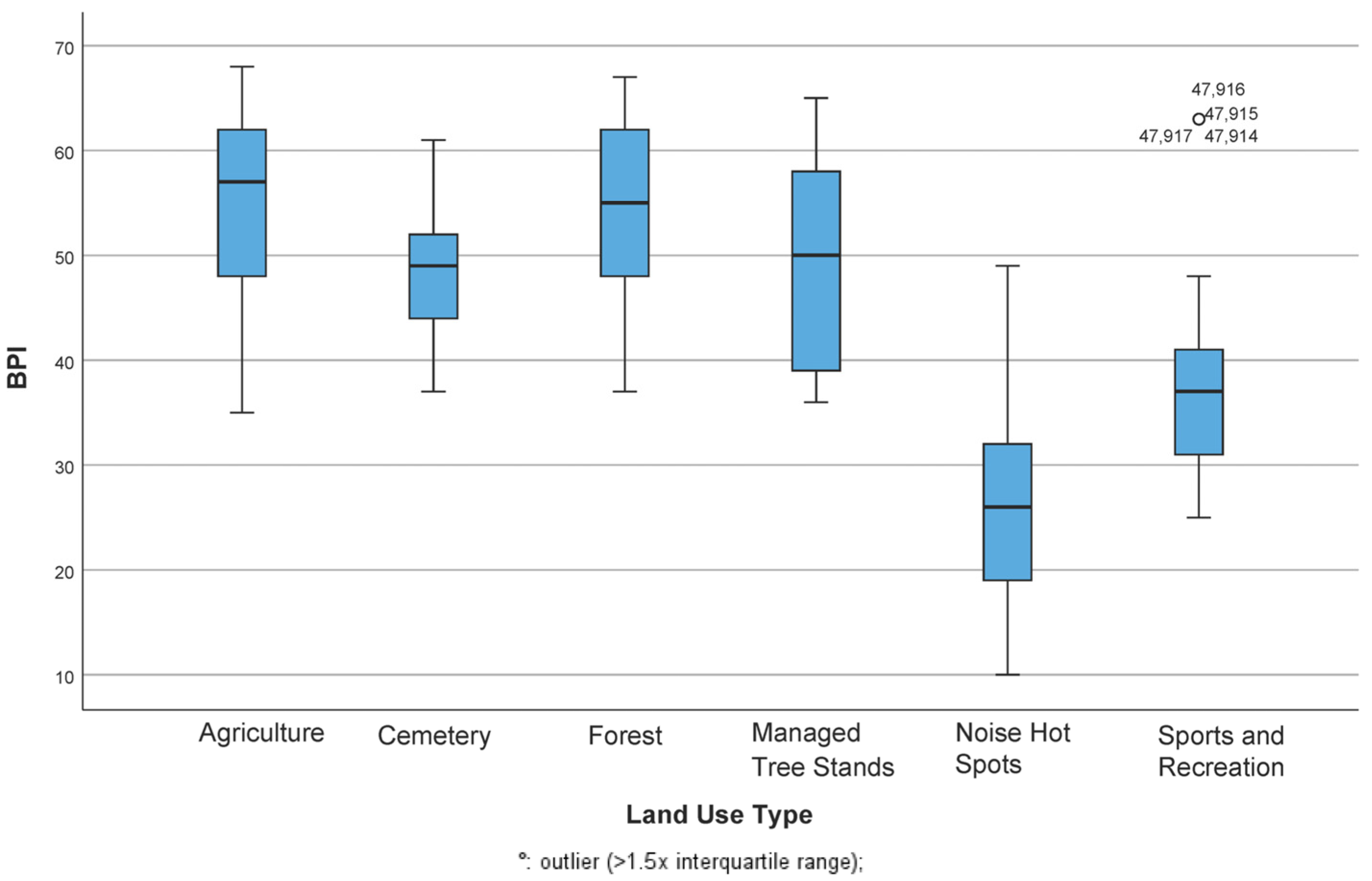
Histograms and boxplots by strata (Figure 5 and Figure 6) show that mean dB(A) values in proposed quiet areas in Dortmund are on average 18.5 to 21 dB(A) lower than the top 23 noise hot spots. On average, forests are the quietest at 45.9 dB(A), followed by cemetery at 46.2 dB(A), managed tree stands at 46.3 dB(A), agriculture at 47.3 dB(A), and sports and recreation at 48.4 dB(A). Outliers are most concentrated in managed tree stands and have the largest spread in agriculture, but since outliers only represent 0.001% of datapoints, then they are not numerous enough to appear in the following diel patterns. Based on the descriptive statistics summary, three quiet area groups emerge: (1) forest and managed tree stands as core quiet areas with upper quartile limits at 60 dB(A), (2) cemeteries and sports and recreation with slightly higher mean dB(A) values and upper quartiles to 65 dB(A), and (3) agriculture with the highest mean dB(A) values and most variance in upper and lower quartiles and outliers. Hot spots predictably have higher mean values but also a different distribution than all quiet area strata, with outliers at the upper and lower ends of quartiles and a right skewed distribution platykurtic in the upper quartile and leptokurtic in the lower quartile.
3.2. Diel Pattern Analysis
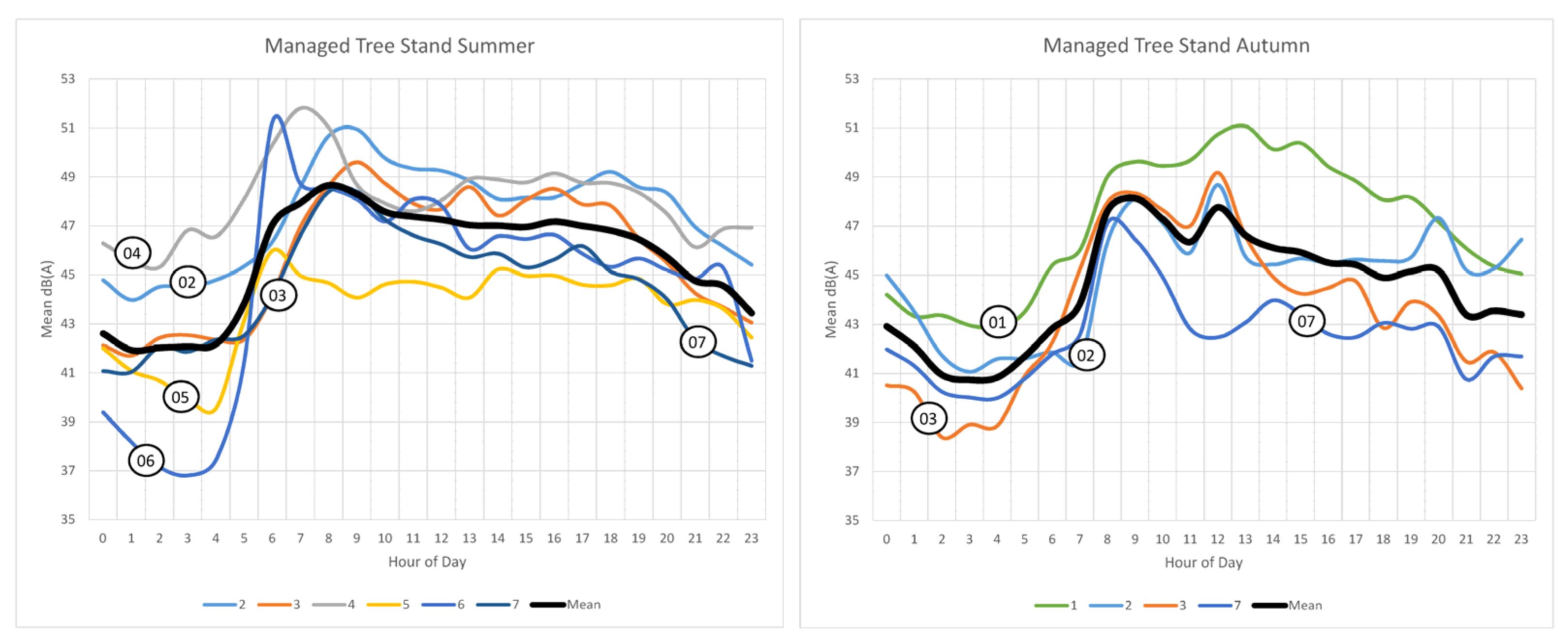
3.2.1. Forest and Managed Tree Stands
Springtime in forests and managed tree stands (Figure 7 and Figure 8) is punctuated with an explosion of sound between 4:00 and 6:00 that continues in a slight downward trend until a dB(A) bump at 22:00. The quietest part of the night is right before 4:00 and nighttime amplitude varies by as much as 10 dB(A) and daytime by 5 dB(A) across strata, with site 31 (forest interior) and 52 (forest edge near highway) as example upper and lower outliers. In comparison to spring, the summer diel patterns include a second or delayed peak around 8:00 (sites 47, 49, 31) and increased outliers above and below the mean; the abrupt end to the spring day at 22:00 then presents a gradual decrease to the deep quiet at 3:00. In the autumn, the double morning peak is delayed to 12:00, after which decibels decline more rapidly than in autumn or summer, and night is quiet except for location 43, with a peak at 4:00. There are only 140 observations with outliers over 70 dB(A), or 0.001%.
3.2.2. Cemetery and Sports and Recreation
Spring in cemeteries is clearly similar to forests, which is unsurprising since these sites are generally forested (Figure 9). The louder quartile range in cemetery observations is explained mostly by site 26 in the summer next to a state road and a highway where the dB(A) peaks at 8:00 and 15:00 to 17:00 are due to traffic. Peaks at these hours are also observed in summer (47) and autumn (43, 20) in forests and all managed tree stands in autumn. This peak is explained by construction noise at site 47 based on our field data sheet, but in the other sites it may indicate a general increase in sound transmissivity through tree stands when trees are mostly defoliated. In autumn site 01, a cemetery located in a village near a school peaks between 13:00 and 15:00 and then reduces thereafter, which could be explained by the end of school and child pickup.
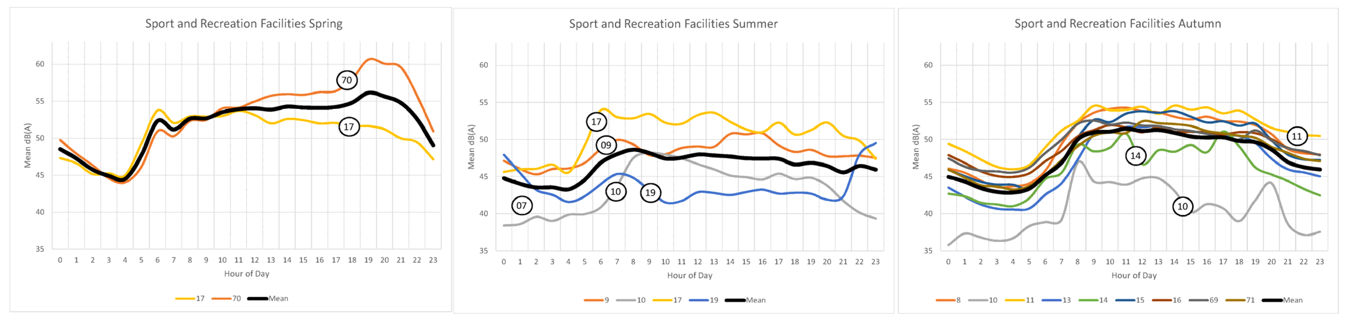
At sports and recreation sites, spring and summer mornings begin at either 6:00 or between 8:00 and 9:00, indicating that some sites experience the morning avifauna chorus and some are more influenced by morning traffic (Figure 10). During the day, these sites experience many ups and downs and some have a dB(A) bump at dusk and some recede gradually often late into the night. This pattern is most likely indicative of sport practices throughout the day and games or practices under lights in the evening. Site 19, a green area in a small community with both sport facilities and a forested cemetery, exhibits increased dB(A) at night versus daytime hours. This could be explained by intensive public use for sport and recreation into the late summer evening, contrasting daytime quietness in the forested cemetery that is not in the immediate proximity of road or rail transport. The autumn diel pattern in sports and recreation is a mix of all patterns and seasons from previously discussed land uses, containing morning peaks at 6:00 and 8:00, a constant sound pressure throughout the day, and then a gradual reduction after 20:00 but without a deep night quietness. This response can be explained by the active use of such facilities in a time of year with reasonably good weather and temperature, situated in relative proximity to roadways but also containing significant forested vegetation stands that include dawn and dusk chorus.
3.2.3. Agriculture
Mean dB(A) values in agriculture strata (Figure 11) are similar to forests, managed tree stands, and cemeteries, but these sites contain significant outliers in spring and summer where dB(A) balloons at sites 54, 55, 57, 59, and 63. These sites are all clustered in the northeast or southeast of Dortmund and appear to be impacted by immediate rail or highway noise over 55 dB(A) (Figure 2). Diel patterns indicate that agricultural land is generally quiet with the presence of dawn and dusk chorus, overlain by continual incursions of transport noise that wash over the low vegetation or open agricultural fields, especially towards the evening.
3.2.4. Noise Hot Spots
Noise hot spots (Figure 12) follow two basic diel patterns, either (1) the presence of a dawn and dusk chorus with a peak in late afternoon, or (2) no apparent presence of dawn or dusk chorus with a strong parabolic form that peaks in late afternoon and recedes slowly to 3:00. Outliers below the mean dB(A) include site 79 (next to a highway but behind a 5 m sound wall), sites 85 and 87 (near major rail and highways but also surrounded by forested vegetation), and site 96 (at the southwest end of the Dortmund airport on a hilltop surrounded by open space and farmland). Outliers above the mean dB(A) include site 76 (Dortmund inner-city road ring) and 78 (main highway artery south out of Dortmund).
3.3. Biophony Power Index
The importance of the temporal dimension is easily seen in the diel patterns, but without information regarding the sound source it is hard to know if dB(A) peaks represent biophony or anthrophony. Thus, we turn to the biophony power index (BPI) maps to help explain the sound source and outlier observations (Figure 13, Figure 14, Figure 15 and Figure 16).
3.3.1. Biophony Power Index 3:00 to 7:59 (Dawn)
In the dawn hours, we find biophony dominated environments (BPI 15–19) in Dortmund south, southeast, and east, where the largest proportion of forested strata is located (Figure 13). Even though a main rail line bisects two large quiet area patches in the east, it does not seem to disturb the propagation of biophony. In the north and west of Dortmund, we find moderate biophonic environments (BPI 11–14), where a matrix of large agricultural lands and forest patches is interspersed with small village centers and crossed by highways. The Dortmund inner-city is clearly distinguished as a large anthrophony dominated area (BPI 2–8) stretching out north, south, east, and west along transport routes. The area between the anthrophony dominated city center and biophony dominated periphery is a zone of balanced anthrophony and biophony characterized mostly by lower rise residential and mixed use land and villages, and large tracts of industry-, agriculture-, or transport-related land uses.
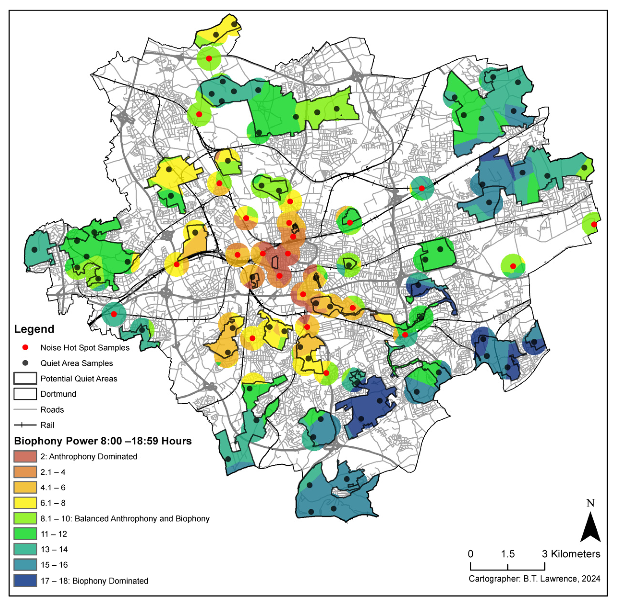
3.3.2. Biophony Power Index 8:00 to 18:59 (Day)
During the day, BPI remains constant in the southeast periphery of Dortmund (BPI 15–19) and reduces in the eastern, south, and southwest periphery (BPI 8–14) (Figure 14). In the south and southwest periphery, the influence of the highway in sites 47, 52 (forest summer), 60 (agriculture summer), and 29 (forest spring) appears to decrease the BPI (Figure 3). Although not near highways, sites 1, 24, and 14 in the city quarter Hombruch (Figure 2) shift from balanced biophony and anthrophony at dawn to anthrophony dominance during the day, explainable by increases in rail transport and general auto-oriented movement of daily commuters to and from Hombruch. Anthrophony dominance also increases during the day in Innenstadt Nord, West, and Ost (city quarter labels in Figure 2). Very little change from dawn to day is observed in the west, but in the north (Mengede), the daytime BPI of sites 53, 27, 80, and 82 increases, possibly attributed to the German highway transport logistics regulations that force large trucks to travel during night and dawn hours.
3.3.3. Biophony Power Index 20:00 to 21:59 (Evening)
Evening hours are anthrophony dominated in the Dortmund Innenstadt quarters (Figure 15). Especially relevant are the increase in anthrophony dominance along the southern highway and northeast rail routes of Innenstadt Ost and Nord, respectively, likely due to the daily road and rail commute. BPI increases in the large forested patches in the south, southeast, and eastern periphery of the city, confirming an avifaunal evening chorus as seen in the diel patterns. In Lütgendortmund on the western periphery, there is very little change in BPI from day to evening, but in the north, the return of commuter traffic is observed with decreases in BPI at transport hot spots 80, 82, and 89.
3.3.4. Biophony Power Index 22:00 to 2:59 (Night)
Night has the greatest reduction in dB(A) amongst all strata and is characterized across much of Dortmund as balanced anthrophony and biophony (BPI 6–12) (Figure 16). Notably, night BPI significantly reduces in forested areas in Hörde, Hombruch, and Aplerbeck to the south and southeast of the city, reflected in forest diel patterns where db(A) decreases. BPI at night is highest in forest and agricultural sites on the east periphery of the city (sites 6, 55, 58, 63). In the city, anthrophony dominance shrinks to only Innenstadt West (sites 77, 76, 83, 89, 9) and Nord (91, 74, 93). In the western periphery Lütgendortmund, BPI reduces equally across all strata.
3.3.5. Association between BPI, dB(A), and Ecoacoustic Factors
The correlation between BPI, dB(A), and the seven ecoacoustic factors included in the BPI model (Table 3) indicates a strong positive correlation with NDSI (r = 0.606 **), moderate positive and negative correlations with NP (r = 0.425 **), dB(A) (r = −0.548 **), M (r = −0.579 **), and weak negative and positive correlations with BIO (r = −0.303 **), Ht (r = 0.275 **). TFSDBird and ACI have only very weak, but significant, correlations with BPI. The findings confirm that dB(A), NDSI, NP, and M are the primary grouping of acoustic indices associated with biophony and anthrophony sonotopes urban acoustic environment.
The index BIO, which decreases as BPI increases, is inverse to expected performance. A boxplot of BIO distribution by land use type (Figure 17) shows that noise hot spots have higher BIO values than all other quiet areas, presumably because the frequency range of automobiles overlaps the biophonic frequency range in the BIO index (2 kHz–8 kHz). To understand this seemingly confounding result, a post hoc analysis of isolated noise hot spots and quiet areas resulted in a weak positive correlation between BPI and BIO (r = 0.179 **) in a restricted sample of only quiet areas (n = 201, 230) and a weak negative correlation between BIO and BPI (r = −0.195 **) in a restricted sample of only noise hot spots (n = 81, 534) (Appendix A).
3.3.6. Spatial Associations with BPI
As a final analysis step, we look at the association of BPI and spatial factors in Table 4 and Figure 18. BPI has moderate or weak positive associations with distance to rail (r = 0.567 **), road (r = 0.322 **), highway noise (r = 0.271 **), and patch size (r = 0.391 **) and moderate negative associations with distance to water (r = −0.498 **). The association to number of plant associations was very weak but still significant (r = 0.157 **).
BPI appears to clarify the descriptive statistics and diel pattern findings when summarized by land use, placing forests, agriculture, and managed tree stands at the top of the BPI ranking, followed by cemeteries, then sports and recreation, and finally noise hot spots with the lowest BPI rankings. This ranking can be described as a gradient from natural land cover strata to strata with increasingly planned human activity.
4. Discussion
4.1. Temporal and Seasonal dB(A) Patterns amongst Quiet Areas and Noise Hot Spots
Seasonally, quiet areas in spring appear to be the most similar across all strata, characterized by the dawn and dusk chorus, an active daytime, and quiet nights. In the summer, dawn biophony is still visible in most strata but the mean amplitude difference between deep night and the dawn chorus peak reduces by 2 to 4 dB(A). Past studies in the neighboring city of Bochum identified increases in the spring normalized mean power spectrum between frequencies of 3–9 kHz that subsequently reduces, supporting our findings [87]. At sports and recreation facilities, autumn acoustic environments are clearly very active from morning until night, most likely explained by the well-known popularity of soccer in Dortmund, with practices running from morning until well in the evening under lights.
The quiet area selection criteria used in Dortmund based on LDEN [67] and spatial factors [13,22] successfully identified areas with significantly lower mean dB(A) values. However, from the diel pattern analysis, we found that the quiet areas themselves can be quite different depending on land use and time of day. Especially, dawn and dusk (20:00 to 22:00) contain variation amongst strata not identifiable in LDEN or noise maps summarized as single exposure values [67]. The diel patterns in this study reinforce the presence of dawn and dusk chorus in urban forests that is masked in mixed use areas [62].
Although LDEN is a useful determination of noise exposure, it does not contain enough time scales to characterize the temporal variation of quiet area acoustic environments. As a matter of fact, none of the quiet area identification best practices such as Ln variations, functional land uses, distance from motorways, size, or visual indicators [13] include temporal considerations detailed enough to identify the variations in dawn and dusk chorus in potential quiet areas as identified in this study. Psychoacoustic studies could be sensitive enough for this differentiation, but they must then be designed with both temporal and spatial dimensions in mind, further increasing the complexity of such studies and increasing the difficulty of recruiting enough participants to make results statistically valid. In this case, the use of automated empirical observations at all hours of the day coupled with psychoacoustic laboratory experiments [88] could be useful.
4.2. Spatio-Temporal Distribution of Biophony and Anthrophony
Without frequency information, it is difficult to assign changes in amplitude information in diel patterns to biophony or anthrophony, but the BPI can overcome this limitation. The BPI reveals that rapid dB(A) increases from 3:00 to 8:00 in the forested quiet areas in the south and southeast of Dortmund are characterized by biophonic dominance and the absence of anthrophony. Only via the subdivision of the ‘night’ time scale was this spatio-temporal phenomena identifiable. Had we modelled BPI from 22:00 to 8:00 as in LDEN, it would have appeared that these areas could be characterized with nighttime biophonic sounds and thus contradicted the diel pattern findings that dB(A) in forested land uses drops off after 22:00. This subdivision also showed that 22:00 to 3:00 is truly the quietest time in Dortmund and, aside from agricultural areas on the east edge of Dortmund, is generally balanced between biophony and anthrophony.
Of equal interest to the distribution of high BPI values are the low BPI value distributions representing a large anthrophony dominated sonotope. Predictably, anthrophony is distributed in the urban core neighborhoods of Dortmund. Our findings support past studies that found a gradient of anthrophony to biophony along an urban gradient from inner city to peri-urban edge and natural areas [35,57,89]. This study adds the observation that anthrophony expands during the daytime hours of 8:00–19:00, reaches its peak from 19:00 to 22:00 being concentrated in the inner-city and along transport routes, and then drastically recedes between 22:00 and 3:00 to only the urban core neighborhood nuclei and highway transport corridors.
Although there are quiet areas designated in and on the direct periphery of the urban core, these areas are, at best, balanced between anthrophony and biophony (BPI 10) and often trend toward anthrophony dominance (BPI 3–8). This finding highlights the difference between urban green spaces that have lower dB(A) values than surrounding noise-polluted areas with some beneficial visual elements (i.e., green) versus large natural areas on the urban periphery with actual resources of biophonic quality that facilitate psychological recovery from noise pollution and connection with natural circadian sound rhythms. At best, inner city green spaces such as 70, 12, 68, 69, 71, 16, 11, and 15 function as respites from noise and anthrophony between the hours of 19:00 and 8:00 with noise-polluted edges, as seen in Figure 2.
To date, there are few, if any, comparable studies to refer or relate to the BPI findings, emphasizing the need for continued study of quiet areas across broad urban regions. This also implies that the unique land use stratified automated aural sampling procedures [63] of temporally dense big data sets are a unique geographic sampling approach that can deliver a higher resolution understanding of the spatio-temporal urban acoustic environment not possible in studies with limited sample sizes [18,29,36,41,72,83,90,91,92,93,94,95].
The selection of factors for the BPI procedure are defended as a meta-study selection based on findings from the past literature [35,57,69,88]. Correlation of BPI with its constituent factors supports the findings of these past studies that dB(A), NDSI, M, and NP are useful for differentiation of anthrophonic and biophonic acoustic environments. As expected based on previous studies reporting bias in the BIO index [57,62], the BIO correlation direction is confounding when analyzed amongst all observations but works when observations are restricted to known noise-polluted areas and quiet areas. This finding pinpoints exactly the nature of bias of the BIO index related to its use in the urban acoustic environment, and it is a double edged sword; it works as expected to compare quiet areas and green infrastructure as long as the sample does not include noise-polluted areas but cannot differentiate between anthrophony and biophony in datasets where the influence is unknown. Thus, BIO remains useful to evaluate the biophonic quality of areas that are already known to not be noise polluted, such as quiet areas in this study, but likely increases the BPI value artificially in anthrophony dominated areas. Nonetheless, the use of the MCDA approach offsets this bias by virtue of multiple indicators to maintain a reasonable outcome of biophony and anthrophony distribution.
Although TFSDBird had only weak associations with BPI, it positively correlates with biophony in quiet areas and negatively in noise hot spots; thus, it may be useful as a screening tool in urban environments to differentiate between patches with morning chorus and patches without a morning chorus, or biophony vs. anthrophony dominance. This virtue is likely due to the nature of the TFSDBird index that focuses on 125 ms variations in time and frequency dimensions in the 4 kHz band. Further study of TFSDBird performance in urban environments is a promising research avenue.
4.3. Association of BPI and Spatial Factors
BPI results by sample strata (Figure 18) provide a completely different picture than dB(A) alone (Figure 6) and add to understanding the distribution of diel patterns via mapping, which is otherwise only possible from cross-referencing diel pattern graphs with sample locations such as in Figure 2. The BPI model seems like a promising approach to understand the biophonic quality of quiet areas. BPI mapping is a compliment to noise mapping in German noise action plans. Here, a two tiered process for quiet area distinction can be seen, where (1) the spatial selection criteria, as the currently recommended best practice in the EU, are applied to identify relatively large areas away from noise pollution, and (2) empirical sound data collection and subsequent BPI mapping differentiate the spatial-temporal biophonic quality of quiet areas from step 1 to further understand the acoustic resources of quiet areas and justify their selection, as required by German law [19].
Correlations of BPI, distances to noise sources, and patch size reinforce the usefulness of spatial factors as primary screening criteria to identify quiet areas. Moderate positive correlations of BPI to water and a weak but significant correlation to number of vertical vegetation layers indicate that habitat quality measures may play a role in biophonic quality, an aspect that should be considered more intensively in follow-up studies. Finally, the BPI and spatial findings support the conceptual framework of soundscape ecology that anthrophony and biophony sonotopes can be mapped and are related to spatial phenomena [27,28]. More importantly, we find heterogeneity in the spatial distribution of soundtopes across large-scale urban acoustic environments.
4.4. Limitations of the Study
Quiet area and noise hot spot samples are not distributed equally across all seasons and therefore we chose to make a single BPI model representing the composite results of all seasons. Future studies should seek to sample all sites in all seasons to overcome this limitation. It is also possible that noise hot spots could contain more biophony in spring and summer months not represented in this study since noise hot spot data were collected in fall and winter where avifauna activity is relatively low. Nonetheless, we believe this study is a useful first step towards the development of methods to differentiate biophonic quality in urban environments.
The BPI approach relies on past studies for factor selection. Given the limited study of ecoacoustic indices in the urban environment, this selection is justified. However, further studies are necessary in a wider range of locations to further refine and validate the approach. The strength of the BPI approach, based on the rational principle of dominance, is that it is robust to the effect of bias in any single factor, such as observed in this study with BIO.
The BPI results are only valid to a confidence level of 80% within proposed quiet areas and around sampled noise hot spots. Future studies could incorporate an estimate of the variance of prediction between two interpolated points to spatially mask areas where the variance of kriging interpolation is too high for prediction. To accommodate for this effect in the interpolated surfaces, all statistics in this study are presented for the sample points themselves and are not based on any interpolated values.
5. Conclusions
This work presents a multi-season case study of 70 quiet areas and 23 hot spots in the city of Dortmund, Germany. Using descriptive statistics, we find that quiet areas are on average 20 dB(A) quieter than noise hot spots. Diel patterns illustrate that dB(A) across quiet areas and noise hot spots differs depending on the time of day, land use, and season. The use of a biophony power index (BPI) to rank and combine eight composite acoustic indices is presented and the BPI is mapped out across Dortmund according to time scales corresponding to LDEN. Diel patterns and correlations indicate that biophonic sonotopes are especially prevalent in large patches of forest, managed tree stands, and agriculture, during the dawn and dusk hours in spring, away from rail and road transport, in proximity to water and with a larger number of vegetated layers in the plant community. These areas are distributed in the southern and eastern portions of Dortmund. Anthrophonic sonotopes are predictably distributed in the urban core neighborhoods and expand and contract slightly throughout the day along transport corridors. The BPI approach compliments LDEN-based noise mapping by providing a spatio-temporal dimension to biophony and anthrophony distribution across an urban region. With further study and refinement, we argue that such an approach could be a useful addition to quiet area identification and qualification in European or German noise action plans.
Author Contributions
Conceptualization, B.T.L. and A.F.; methodology, B.T.L.; software, B.T.L.; validation, B.T.L., A.F., K.S. and D.H.; formal analysis, B.T.L. and D.H.; investigation, B.T.L., D.H., K.S. and D.G.; resources, B.T.L.; data curation, K.S. and D.H.; writing—original draft preparation, B.T.L.; writing—review and editing, B.T.L., A.F., D.H., K.S. and D.G.; visualization, B.T.L. and D.H.; supervision, B.T.L. and D.G.; project administration, B.T.L. and D.G.; funding acquisition, B.T.L., A.F. and D.G. All authors have read and agreed to the published version of the manuscript.
Funding
This research was funded by a grant from the City of Dortmund Environmental Office, 44135 Dortmund, Germany in 2022.
Data Availability Statement
The original contributions presented in the study are included in the article, further inquiries can be directed to the corresponding author.
Acknowledgments
The authors wish to thank the TU Dortmund Spatial Planning A05 Project of 2022/23 for their assistance in the preliminary and explorative analysis of this dataset.
Conflicts of Interest
The authors declare no conflicts of interest.
Appendix A
- 1.
- Kolmogorov–Smirnov test of normality reveals that all sound factors have p < 0.001 and thus significantly deviate from a normal distribution (Table A1).

Table A1.
Kolmogorov–Smirnov test of normality for sound factors.
| Kolmogorov–Smirnov a | |||
|---|---|---|---|
| Statistic | df | Sig. | |
| A Weighted (Mean dB) | 0.125 | 282764 | <0.001 |
| ACI | 0.204 | 282763 | <0.001 |
| TFSDBirds | 0.198 | 282763 | <0.001 |
| BIO | 0.104 | 282763 | <0.001 |
| NP | 0.052 | 282763 | <0.001 |
| NDSI | 0.060 | 282763 | <0.001 |
| M | 0.278 | 282763 | <0.001 |
| Ht | 0.210 | 282763 | <0.001 |
a Lilliefors Significance Correction.
- 2.
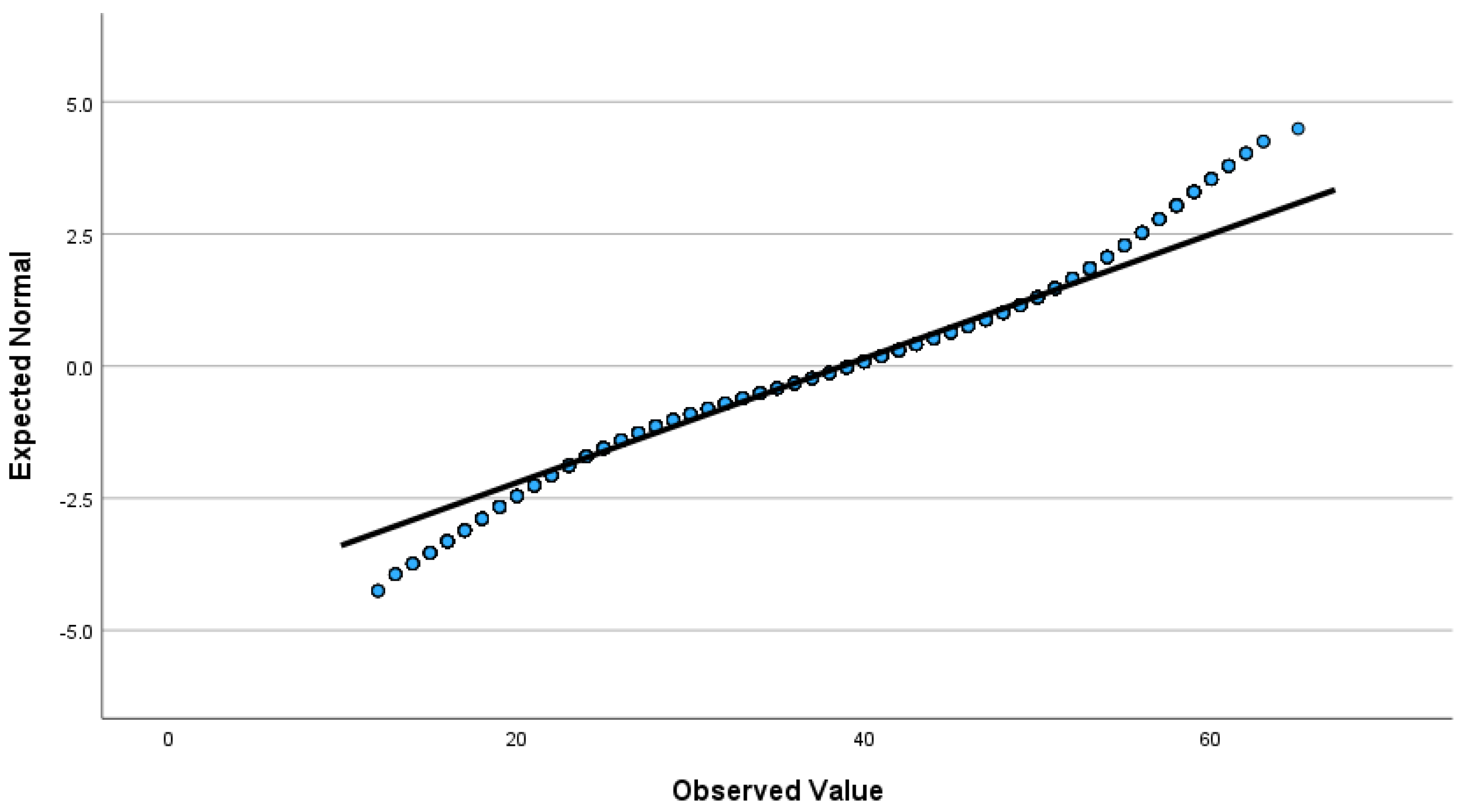
Figure A1.
Normal Q—Q plot of mean dB(A).

Figure A2.
Normal Q—Q plot of ACI.

Figure A3.
Normal Q—Q plot of TFSDBird.

Figure A4.
Normal Q—Q plot of BIO.

Figure A5.
Normal Q—Q plot of NP.

Figure A6.
Normal Q—Q plot of NDSI.

Figure A7.
Normal Q—Q plot of M.

Figure A8.
Normal Q—Q plot of Ht.

- 3.
Table A2.
Spearman’s correlation of BPI and BIO in only quiet areas (n = 201, 230).
| Factor | BIO |
|---|---|
| BPI | 0.179 ** |
** Correlation is significant at the 0.01 level (2-tailed).
Table A3.
Spearman’s correlation of BPI and BIO in only noise hot spots (n = 81, 534).
| Factor | BIO |
|---|---|
| BPI | −0.195 ** |
** Correlation is significant at the 0.01 level (2-tailed).
References
- WHO. Burden of Disease from Environmental Noise: Quantification of Healthy Life Years Lost in Europe. Available online: https://www.euro.who.int/__data/assets/pdf_file/0008/136466/e94888.pdf (accessed on 3 November 2021).
- Fuks, K.; Moebus, S.; Hertel, S.; Viehmann, A.; Nonnemacher, M.; Dragano, N.; Mohlenkamp, S.; Jakobs, H.; Kessler, C.; Erbel, R.; et al. Long-term urban particulate air pollution, traffic noise, and arterial blood pressure. Environ. Health Perspect. 2011, 119, 1706–1711. [Google Scholar] [CrossRef]
- Selander, J.; Nilsson, M.E.; Bluhm, G.; Rosenlund, M.; Lindqvist, M.; Nise, G.; Pershagen, G. Long-term exposure to road traffic noise and myocardial infarction. Epidemiology 2009, 20, 272–279. [Google Scholar] [CrossRef]
- Sörenson, M.; Hvidberg, M.; Anderson, Z.J.; Nordsborg, R.B.; Lillelund, K.G.; Jakobsen, J.; Tjonneland, A.; Overvad, K.; Raaschou-Nielsen, O. Road traffic noise and stroke: A prospective cohort study. Eur. Heart J. 2011, 32, 737–744. [Google Scholar] [CrossRef]
- Kälsch, H.; Hennig, F.; Moebus, S.; Mohlenkamp, S.; Dragano, N.; Jakobs, H.; Memmesheimer, M.; Erbel, R.; Jockel, K.H.; Hoffmann, B. Are air pollution and traffic noise independently associated with atherosclerosis: The Heinz Nixdorf Recall Study. Eur. Heart J. 2014, 35, 853–860. [Google Scholar] [CrossRef] [PubMed]
- Orban, E.; McDonald, K.; Sutcliffe, R.; Hoffmann, B.; Fuks, K.; Dragano, N.; Viehmann, A.; Erbel, R.; Jöckel, K.H.; Pundt, N.; et al. Residential Road Traffic Noise and High Depressive Symptoms after Five Years of Follow-up: Results from the Heinz Nixdorf Recall Study. Environ. Health Perspect. 2016, 124, 578–585. [Google Scholar] [CrossRef]
- Seidler, A.; Schubert, M.; Romero Starke, K.; Hegewald, J. Einfluss des Lärms auf Psychische Erkrankungen des Menschen; Research ID 3717 56 102 0; Umweltbundesamt: Dessau-Roßlau, Germany, 2023; Available online: https://www.umweltbundesamt.de/publikationen/einfluss-des-laerms-auf-psychische-erkrankungen-des (accessed on 21 February 2024).
- Farina, A.; Gage, S.H. (Eds.) Ecoacoustics: The Ecological Role of Sounds, 1st ed.; John Wiley & Sons, Inc.: Hoboken, NJ, USA, 2017; ISBN 9781119230724. [Google Scholar]
- Farina, A. Soundscape Ecology: Principles, Patterns, Methods and Applications; Springer: Urbino, Italy, 2014. [Google Scholar]
- DIN 12913-1; TS I—Acoustics—Soundscape Part 1: Definition and Conceptual Framework. ISO: Geneva, Switzerland, 2014.
- Sueur, J. Sound Analysis and Synthesis with R; Springer International Publishing: Cham, Switzerland, 2018; ISBN 978-3-319-77645-3. [Google Scholar]
- DIN 12913-3; TS III—Acoustics—Soundscape Part 3: Data Analysis. ISO: Geneva, Switzerland, 2019.
- EEA. Good Practice Guide on Quiet Areas; Technical Report 04; European Environmental Agency: Copenhagen, Denmark, 2014. [Google Scholar]
- Gidlöf-Gunnarsson, A.; Öhrström, E. Noise and well-being in urban residential environments: The potential role of perceived availability to nearby green areas. Landsc. Urban Plan. 2007, 83, 115–126. [Google Scholar] [CrossRef]
- Öhrström, E.; Skånberg, A.; Svensson, H.; Gidlöf-Gunnarsson, A. Effects of road traffic noise and the benefit of access to quietness. J. Sound Vib. 2006, 295, 40–59. [Google Scholar] [CrossRef]
- Kaplan, S. The restorative benefits of nature: Toward an integrative framework. J. Environ. Psychol. 1995, 156, 169–182. [Google Scholar] [CrossRef]
- Alvarsson, J.J.; Wiens, S.; Nilsson, M.E. Stress recovery during exposure to nature sound and environmental noise. Int. J. Environ. Res. Public Health 2010, 7, 1036–1046. [Google Scholar] [CrossRef] [PubMed]
- Kang, J.; Yang, W. Acoustic comfort evaluation in urban open public spaces. Appl. Acoust. 2005, 66, 211–229. [Google Scholar] [CrossRef]
- BlmSchG §47d: Act on Protection against Harmful Effects on the Environment Caused by Air Pollution, Noise, Vibrations and Similar Processes (Federal Immission Control Act-BImSchG) § 47d Noise Action Plans. 2008. Available online: https://www.gesetze-im-internet.de/bimschg/__47d.html (accessed on 24 March 2024).
- DIN ISO 12913-2; TS II—Acoustics—Soundscape Part 2: Data Collection and Reporting Requirements. ISO: Geneva, Switzerland, 2018.
- EU Noise Directive 2002/49/EC. END, European Parliament and of the Council of the European Union: Brussels, Belgium, 2002. Revised 3-25-2020. Available online: https://eur-lex.europa.eu/LexUriServ/LexUriServ.do?uri=OJ:L:2002:189:0012:0025:en:PDF (accessed on 24 March 2024).
- Heinrichs, E.; Leben, J.; Cancik, P. Ruhige Gebiete: Eine Fachbroschüre für die Lärmaktionsplanung. Available online: https://www.umweltbundesamt.de/sites/default/files/medien/1410/publikationen/181005_uba_fb_ruhigegebiete_bf_150.pdf (accessed on 24 March 2024).
- Mackenbach, R.; Schneemelcher, O. Lärmaktionsplan der Stadt Dortmund. Zusammenfassung. Stadt Dortmund Umweltamt. 2014. Available online: https://docplayer.org/6959070-Laermaktionsplan-der-stadt-dortmund.html (accessed on 24 March 2024).
- Zänger, K.; Schöller, A. Eu-Umgebunslärm Detaillierter Lärmaktionsplan für den Ballungsraum Bochum. Stadt Bochum Umwelt- und Grünflächenamt. 2015. Available online: https://www.bochum.de/C125830C0042AB74/vwContentByKey/78B01F618DF05904C125853D0038082C/$FILE/Gesamt_Detaillierter_LAP.pdf(accessed on 24 March 2024).
- Kuhlmann, Werner: Laermaktionsplan Essen. Stadt Essen. Essen, Germany. 2021. Available online: https://media.essen.de/media/wwwessende/aemter/59/lrm/laermaktionsplan2021/Laermaktionsplan_2021.pdf(accessed on 24 March 2024).
- Botz, K.; Gatzweiler, M.; Riedel, M.; Schommer, M.; Schüren-Hinkelmann, S. Lärmaktionsplan der Stadt Duisburg. Available online: https://sessionnet.krz.de/duisburg/bi/getfile.asp?id=1651994&type=do (accessed on 24 March 2024).
- Farina, A.; Pieretti, N. A new frontier of landscape research and its application to islands and coastal systems. J. Mar. Isl. Cult. 2012, 1, 21–26. [Google Scholar] [CrossRef]
- Pijanowski, B.C.; Villanueva-Rivera, L.J.; Dumyahn, S.L.; Farina, A.; Krause, B.L.; Napoletano, B.M.; Gage, S.H.; Pieretti, N. Soundscape Ecology: The Science of Sound in the Landscape. BioScience 2011, 61, 203–2016. [Google Scholar] [CrossRef]
- Kang, J.; Yu, L. Factors influencing the sound preference in urban open spaces. Appl. Acoust. 2010, 71, 622–633. [Google Scholar] [CrossRef]
- Liu, J.; Kang, J.; Behm, H.; Luo, T. Effects of landscape on soundscape perception: Soundwalks in city parks. Landsc. Urban Plan. 2014, 123, 30–40. [Google Scholar] [CrossRef]
- Kang, J.; Liu, J. Soundscape Design in City Parks: Exploring the Relationships between Soundscape Composition Parameters and Physical and Psychoacoustic Parameters. J. Environ. Eng. Landsc. Manag. 2014, 23, 102–112. [Google Scholar]
- Orban, E.; Sutcliffe, R.; Dragano, N.; Jöckel, K.-H.; Moebus, S. Residential Surrounding Greenness, Self-Rated Health and Interrelations with Aspects of Neighborhood Environment and Social Relations. J. Urban Health 2017, 94, 158–169. [Google Scholar] [CrossRef] [PubMed]
- Aletta, F.; Kang, J.; Axelsson, Ö. Soundscape descriptors and a conceptual framework for developing predictive soundscape models. Landsc. Urban Plan. 2016, 149, 65–74. [Google Scholar] [CrossRef]
- Sun, K.; de Coensel, B.; Filipan, K.; Aletta, F.; van Renterghem, T.; de Pessemier, T.; Joseph, W.; Botteldooren, D. Classification of soundscapes of urban public open spaces. Landsc. Urban Plan. 2019, 189, 139–155. [Google Scholar] [CrossRef]
- Joo, W.H.; Gage, S.; Kasten, E.P. Analysis and interpretation of variability in soundscapes along an urban?: Rural gradient. Landsc. Urban Plan. 2011, 103, 259–276. [Google Scholar] [CrossRef]
- Jeon, J.Y.; Hong, J.Y. Classification of urban park soundscapes through perceptions of the acoustical environments. Landsc. Urban Plan. 2015, 141, 100–111. [Google Scholar] [CrossRef]
- Aletta, F.; Kang, J. Soundscape approach integrating noise mapping techniques: A case study in Brighton, UK. Noise Mapp. 2015, 2, 1–12. [Google Scholar] [CrossRef]
- Margaritis, E.; Kang, J. Soundscape mapping in environmental noise management and urban planning: Case studies in two UK cities. Noise Mapp. 2017, 4, 87–103. [Google Scholar] [CrossRef]
- Lippold, M.; Lawrence, B.T. Soundscape Planning as a Tool for Urban Planning. In Proceedings of the 23rd International Congress on Acoustics, Integrating 4th EAA Euroregio 2019, Aachen, Germany, 8–13 September 2019; Ochmann, M., Vorländer, M., Fels, J., Eds.; RWTH Publications: Aachen, Germany, 2019. ISBN 978-3-939296-15-7. [Google Scholar]
- Hao, Z.; Wang, C.; Sun, Z.; van den Bosch, C.K.; Zhao, D.; Sun, B.; Zhao, Y. Soundscape mapping for spatial-temporal estimate on bird activities in urban forests. Urban For. Urban Green. 2020, 57, 126822. [Google Scholar] [CrossRef]
- Margaritis, E.; Kang, J.; Filipan, K.; Botteldooren, D. The influence of vegetation and surrounding traffic noise parameters on the sound environment of urban parks. Appl. Geogr. 2018, 94, 199–212. [Google Scholar] [CrossRef]
- Chitra, B.; Jain, M.; Chundelli, F.A. Understanding the soundscape environment of an urban park through landscape elements. Environ. Technol. Innov. 2020, 19, 100998. [Google Scholar] [CrossRef]
- Bradfer-Lawrence, T.; Gardner, N.; Bunnefeld, L.; Bunnefeld, N.; Willis, S.G.; Dent, D.H. Guidelines for the use of acoustic indices in environmental research. Methods Ecol. Evol. 2019, 10, 1796–1807. [Google Scholar] [CrossRef]
- Challeat, S.; Gasc, A.; Farrugia, N.; Froidevaux, J. Silent Cities: A Participatory Monitoring Programme of an Exceptional Modification of Urban Soundscapes. Call for Participation to a Dataset Collection. 2020. Available online: https://renoir.hypotheses.org/files/2020/03/Silent%C2%B7Cities-Project.pdf (accessed on 16 March 2021).
- Boelman, N.T.; Asner, G.P.; Hart, P.J.; Martin, R.E. Multi-Trophic Invasion Resistance in Hawaii: Bioacoustics, Field Surveys, and Airborne Remote Sensing. Ecol. Appl. 2007, 2007, 2137–2144. [Google Scholar] [CrossRef]
- Sueur, J.; Pavoine, S.; Hamerlynck, O.; Duvail, S. Rapid Acoustic Survey for Biodiversity Appraisal. PLoS ONE 2008, 3, e4065. [Google Scholar] [CrossRef] [PubMed]
- Krause, B.; Gage, S.H.; Joo, W. Measuring and interpreting the temporal variability in the soundscape at four places in Sequoia National Park. Landsc. Ecol. 2011, 26, 1247–1256. [Google Scholar] [CrossRef]
- Rodriguez, A.; Gasc, A.; Pavoine, S.; Grandcolas, P.; Gaucher, P.; Sueur, J. Temporal and spatial variability of animal sound within a neotropical forest. Ecol. Inform. 2014, 21, 133–143. [Google Scholar] [CrossRef]
- Towsey, M.; Roe, P.; Wimmer, J.; Williamson, I. The use of acoustic indices to determine avian species richness in audio-recordings of the environment. Ecol. Inform. 2014, 21, 110–119. [Google Scholar] [CrossRef]
- Bradfer-Lawrence, T.; Bunnefeld, N.; Gardner, N.; Willis, S.G.; Dent, D.H. Rapid assessment of avian species richness and abundance using acoustic indices. Ecol. Indic. 2020, 115, 106400. [Google Scholar] [CrossRef]
- Dröge, S.; Martin, D.A.; Andriafanomezantsoa, R.; Burivalova, Z.; Fulgence, T.R.; Osen, K.; Rakotomalala, E.; Schwab, D.; Wurz, A.; Richter, T.; et al. Listening to a changing landscape: Acoustic indices reflect bird species richness and plot-scale vegetation structure across different land-use types in north-eastern Madagascar. Ecol. Indic. 2021, 120, 106929. [Google Scholar] [CrossRef]
- Mammides, C.; Goodale, E.; Dayananda, S.K.; Kang, L.; Chen, J. Do acoustic indices correlate with bird diversity? Insights from two biodiverse regions in Yunnan Province, south China. Ecol. Indic. 2017, 82, 470–477. [Google Scholar] [CrossRef]
- Shamon, H.; Paraskevopoulou, Z.; Kitzes, J.; Card, E.; Deichmann, J.L.; Boyce, A.J.; McShea, W.J. Using ecoacoustics metrices to track grassland bird richness across landscape gradients. Ecol. Indic. 2021, 120, 106928. [Google Scholar] [CrossRef]
- Fuller, S.; Axel, A.C.; Tucker, D.; Gage, S.H. Connecting soundscape to landscape: Which acoustic index best describes landscape configuration? Ecol. Indic. 2015, 58, 207–215. [Google Scholar] [CrossRef]
- Scarpelli, M.D.A.; Ribeiro, M.C.; Teixeira, C.P. What does Atlantic Forest soundscapes can tell us about landscape? Ecol. Indic. 2021, 121, 107050. [Google Scholar] [CrossRef]
- Gasc, A.; Pavoine, S.; Lellouch, L.; Grandcolas, P.; Sueur, J. Acoustic indices for biodiversity assessments: Analyses of bias based on simulated bird assemblages and recommendations for field surveys. Biol. Conserv. 2015, 191, 306–312. [Google Scholar] [CrossRef]
- Fairbrass, A.J.; Rennert, P.; Williams, C.; Titheridge, H.; Jones, K.E. Biases of acoustic indices measuring biodiversity in urban areas. Ecol. Indic. 2017, 83, 169–177. [Google Scholar] [CrossRef]
- Eldridge, A.; Guyot, P.; Moscoso, P.; Johnston, A.; Eyre-Walker, Y.; Peck, M. Sounding out ecoacoustic metrics: Avian species richness is predicted by acoustic indices in temperate but not tropical habitats. Ecol. Indic. 2018, 95, 939–952. [Google Scholar] [CrossRef]
- Devos, P. Soundecology indicators applied to urban soundscapes. In Proceedings of the INTER-NOISE and NOISE-CON Congress and Conference Proceedings, Hamburg, Germany, 21–24 August 2016; pp. 3631–3638. [Google Scholar]
- Gage, S.; Wimmer, J.; Tarrant, T.; Grace, P.R. Acoustic patterns at the Samford Ecological Research Facility in South East Queensland Australia: The peri-urban superSite of the Terrestrial Ecosystem Research NEtwork. Ecol. Inform. 2017, 38, 62–75. [Google Scholar] [CrossRef]
- Depraetere, M.; Pavoine, S.; Jiguet, F.; Gasc, A.; Duvail, S.; Sueur, J. Monitoring animal diversity using acoustic indices: Implementation in a temperate woodland. Ecol. Indic. 2012, 13, 46–54. [Google Scholar] [CrossRef]
- Lawrence, B.T.; Hornberg, J.; Haselhoff, T.; Sutcliffe, R.; Ahmed, S.; Moebus, S.; Gruehn, D. A widened array of metrics (WAM) approach to characterize the urban acoustic environment; a case comparison of urban mixed-use and forest. Appl. Acoust. 2021, 185, 108387. [Google Scholar] [CrossRef]
- Haselhoff, T.; Lawrence, B.; Hornberg, J.; Ahmed, S.; Sutcliffe, R.; Gruehn, D.; Moebus, S. The acoustic quality and health in urban environments (SALVE) project: Study design, rationale and methodology. Appl. Acoust. 2021, 188, 108538. [Google Scholar] [CrossRef]
- Moebus, S.; Gruehn, D.; Poppen, J.; Sutcliffe, R.; Haselhoff, T.; Lawrence, B. Akustische Qualität und Stadtgesundheit—Mehr als nur Lärm und Stille. Bundesgesundheitsblatt Gesundheitsforschung Gesundheitsschutz 2020, 63, 997–1003. [Google Scholar] [CrossRef]
- Israel, G.D. Determining Sample Size; University of Florieda: Gainesville, FL, USA, 1992. [Google Scholar]
- Frücht, A. Bericht über die Umgebungslärmkartierung der IV Stufe im Jahr 2022. 2023. Available online: https://www.dortmund.de/media/p/umweltamt/downloads_umweltamt/umgebungslaerm/Bericht_Umgebungslrmkartierung_der_IV_Stufe_im_Jahr_2022.pdf (accessed on 24 March 2024).
- BlmSchG §47c: Act on Protection against Harmful Effects on the Environment Caused by Air Pollution, Noise, Vibrations and Similar Processes (Federal Immission Control Act-BImSchG) § 47c Noise Maps. 2007. Available online: https://www.gesetze-im-internet.de/bimschg/__47c.html. (accessed on 24 March 2024).
- LANUV. Biotopkataster NRW; LANUV, Landesamt für Natur, Umwelt und Verbraucherschutz Nordrhein-Westfalen: Düsseldorf, Germany, 2023. [Google Scholar]
- Lawrence, B.T.; Ahmed, S.; Sutcliffe, R.; Poppen, J.; Moebus, S.; Gruehn, D. A widened array of metrics (WAM) approach to charactarize urban sound environments: The example in SALVE. In Proceedings of the 23rd International Congress on Acoustics, Integrating 4th EAA Euroregio 2019, Aachen, Germany, 8–13 September 2019; Ochmann, M., Vorländer, M., Fels, J., Eds.; RWTH Publications: Aachen, Germany, 2019. ISBN 978-3-939296-15-7. [Google Scholar]
- Gasc, A.; Sueur, J.; Jiguet, F.; Devictor, V.; Grandcolas, P.; Burrow, C.; Depraetere, M.; Pavoine, S. Assessing biodiversity with sound: Do acoustic diversity indices reflect phylogenetic and functional diversities of bird communities? Ecol. Indic. 2013, 25, 279–287. [Google Scholar] [CrossRef]
- Pieretti, N.; Farina, A.; Morri, D. A new methodology to infer the singing activity of an avian community: The Acoustic Complexity Index (ACI). Ecol. Indic. 2011, 11, 868–873. [Google Scholar] [CrossRef]
- Aumond, P.; Can, A.; de Coensel, B.; Botteldooren, D.; Ribeiro, C.; Lavandier, C. Modeling soundscape pleasantness using perceptual assessments and acoustic measurements along paths in urban context. Acta Acust. United Acust. 2017, 12, 50–67. [Google Scholar] [CrossRef]
- Gontier, F.; Lavandier, C.; Aumond, P.; Lagrange, M.; Petiot, J.-F. Estimation of the Perceived Time of Presence of Sources in Urban Acoustic Environments Using Deep Learning Techniques. Acta Acust. United Acust. 2019, 105, 1053–1066. [Google Scholar] [CrossRef]
- Wildlife Acoustics. Kaleidoscope; Wildlife Acoustics: Maynard, MA, USA, 2021. [Google Scholar]
- Hopkins, L.D. Methods for Generating Land Suitability Maps: A Comparative Evaluation. J. Am. Inst. Plan. 1977, 43, 386–400. [Google Scholar] [CrossRef]
- Malczewski, J. On the Use of Weighted Linear Combination Method in GIS: Common and Best Practice Approaches. Trans. GIS 2000, 4, 5–22. [Google Scholar] [CrossRef]
- Greco, S.; Matarazzo, B.; Slowinski, R. Decision Rule Approach. In Multiple Criteria Decision Analysis: State of the Art Surveys, 2nd ed.; Greco, S., Ehrgott, M., Figueira, J.R., Eds.; Springer: New York, NY, USA; Heidelberg, Germany; Dordrecht, The Netherlands; London, UK, 2016; p. 497. ISBN 9781493930944. [Google Scholar]
- Greco, S.; Ehrgott, M.; Figueira, J.R. (Eds.) Multiple Criteria Decision Analysis: State of the Art Surveys, 2nd ed.; Springer: New York, NY, USA; Heidelberg, Germany; Dordrecht, The Netherlands; London, UK, 2016; p. 552. ISBN 9781493930944. [Google Scholar]
- Lavandier, C.; Aumond, P.; Can, A. (Eds.) Urban Sensor Network for Characterizing the Sound Environment in Lorient (France) through an Automatic Assessment of Traffic, Voice and Bird Presence Ratios; European Congress on Noise Control Engineering (EuroNoise): Madeira, Portugal, 2021. [Google Scholar]
- Krige, D.G. A statistical approach to some basic mine valuation problems on the Witwatersrand. J. S. Afr. Inst. Min. Metall. 1951, 52, 201–203. [Google Scholar]
- Farina, A.; Pieretti, N. Sonic environment and vegetation structure: A methodological approach for a soundscape analysis of a Mediterranean maqui. Ecol. Inform. 2014, 21, 120–132. [Google Scholar] [CrossRef]
- Can, A.; Dekoninck, L.; Botteldooren, D. Measurement network for urban noise assessment: Comparison of mobile measurements and spatial interpolation approaches. Appl. Acoust. 2014, 83, 32–39. [Google Scholar] [CrossRef]
- Tsai, K.-T.; Lin, M.-D.; Chen, Y.-H. Noise mapping in urban environments: A Taiwan study. Appl. Acoust. 2009, 70, 964–972. [Google Scholar] [CrossRef]
- Lawrence, B.T.; Frücht, A.; Sievers, L.; Ammerahl, V.; Boegner, M.; Brockmann, C.; Buran, F.; Hartung, N.; Heying, D.; Jäkel, H.; et al. (Eds.) Quiet Areas in the Ruhr Region; Poster Presentation; Urban Sound Symposium: Barcelona, Spain, 2023. [Google Scholar]
- Spearman, C.E. The proof and measurement of association between two things. Am. J. Psychol. 1904, 15, 72–101. [Google Scholar] [CrossRef]
- Bühl, A. SPSS 20: Einführung in Die Moderne Datenanalyse, 13th ed.; Pearson Studium—Scientific Tools; Pearson: Benelux, The Netherlands, 2012. [Google Scholar]
- Haselhoff, T.; Braun, T.; Hornberg, J.; Lawrence, B.T.; Ahmed, S.; Gruehn, D.; Moebus, S. Analysing Interlinked Frequency Dynamics of the Urban Acoustic Environment. Int. J. Environ. Res. Public Health 2022, 19, 15014. [Google Scholar] [CrossRef] [PubMed]
- Lawrence, B.T.; Hornberg, J.; Schröer, K.; Djeudeu, D.; Haselhoff, T.; Ahmed, S.; Moebus, S.; Gruehn, D. Linking ecoacoustic indices to psychoacoustic perception of the urban acoustic environment. Ecol. Indic. 2023, 155, 111023. [Google Scholar] [CrossRef]
- Dein, J.; Rüdisser, J. Landscape influence on biophony in an urban environment in the European Alps. Landsc. Ecol. 2020, 35, 1875–1889. [Google Scholar] [CrossRef]
- Berengier, M.; Lavandier, C.; Raimbault, M. Ambient sound assessment of urban environments: Field studies in two French cities. Appl. Acoust. 2003, 64, 1241–1256. [Google Scholar] [CrossRef]
- Drake, C.; Viollon, S.; Lavandier, C. Influence of visual setting on sound ratings in an urban environment. Appl. Acoust. 2002, 63, 493–511. [Google Scholar] [CrossRef]
- Rychtarikova, M.; Vermeir, G.; Domecka, M. The Application of the Soundscape Approach in the Evaluation of the Urban Public Spaces. J. Acoust. Soc. Am. 2008, 123, 3810. [Google Scholar] [CrossRef]
- Jia, Y.; Ma, H.; Kang, J.; Wang, C. The preservation value of urban soundscape and its determinant factors—ScienceDirect. Appl. Acoust. 2020, 168, 107430. [Google Scholar] [CrossRef]
- Axelsson, Ö.; Nilsson, M.E.; Hellström, B.; Lundén, P. A field experiment on the impact of sounds from a jet-and-basin fountain on soundscape quality in an urban park. Landsc. Urban Plan. 2014, 123, 49–60. [Google Scholar] [CrossRef]
- Klein, E.; Chapple, S.; Fainberg, J.; Magill, C.; Parker, M.; Raab, C.; Silvertown, J. Capturing the sounds of an urban greenspace. Int. Arch. Photogramm. Remote Sens. Spat. Inf. Sci. 2018, XLII-4/W11, 19–26. [Google Scholar] [CrossRef]
Figure 1.
Interpretation of sound source categories as anthrophony or biophony in step 3 of the soundscape mapping process (Adapted from [38]).
Figure 1.
Interpretation of sound source categories as anthrophony or biophony in step 3 of the soundscape mapping process (Adapted from [38]).

Figure 2.
Distribution of quiet areas in relation to LDEN in the City of Dortmund (author’s own work, with proposed quiet areas, residential parcels and LDEN data provided by the City of Dortmund).
Figure 2.
Distribution of quiet areas in relation to LDEN in the City of Dortmund (author’s own work, with proposed quiet areas, residential parcels and LDEN data provided by the City of Dortmund).

Figure 3.
Sample clusters, quiet area and hot spot samples including sample identification number (ID) (Author’s own work, with roads and potential quiet area boundaries provided by City of Dortmund).
Figure 3.
Sample clusters, quiet area and hot spot samples including sample identification number (ID) (Author’s own work, with roads and potential quiet area boundaries provided by City of Dortmund).

Figure 4.
Biophony Power Index spatial mapping process.

Figure 5.
Histograms of Mean dB(A) by land use type on X-axis with number (#) of observations on Y-axis.
Figure 5.
Histograms of Mean dB(A) by land use type on X-axis with number (#) of observations on Y-axis.

Figure 6.
Boxplots of dB(A) by land use strata.

Figure 7.
Forest diel pattern analysis by season.

Figure 8.
Managed tree stand diel pattern analysis by season.

Figure 9.
Cemetery diel pattern analysis by season.

Figure 10.
Sports and recreation facilities diel pattern analysis by season.

Figure 11.
Agriculture diel pattern analysis by season.

Figure 12.
Noise hot spot diel pattern analysis by season.

Figure 13.
Biophony power index (BPI) distribution from 3:00 to 7:59 hours (Author’s own work, with roads and potential quiet area boundaries provided by City of Dortmund).
Figure 13.
Biophony power index (BPI) distribution from 3:00 to 7:59 hours (Author’s own work, with roads and potential quiet area boundaries provided by City of Dortmund).

Figure 14.
Biophony power index (BPI) distribution from 8:00 to 18:59 hours (Author’s own work, with roads and potential quiet area boundaries provided by City of Dortmund).
Figure 14.
Biophony power index (BPI) distribution from 8:00 to 18:59 hours (Author’s own work, with roads and potential quiet area boundaries provided by City of Dortmund).

Figure 15.
Biophony power index (BPI) distribution by time from 19:00 to 21:59 hours (Author’s own work, with roads and potential quiet area boundaries provided by City of Dortmund).
Figure 15.
Biophony power index (BPI) distribution by time from 19:00 to 21:59 hours (Author’s own work, with roads and potential quiet area boundaries provided by City of Dortmund).

Figure 16.
Biophony power index (BPI) distribution by time from 22:00 to 2:59 hours (Author’s own work, with roads and potential quiet area boundaries provided by City of Dortmund).
Figure 16.
Biophony power index (BPI) distribution by time from 22:00 to 2:59 hours (Author’s own work, with roads and potential quiet area boundaries provided by City of Dortmund).

Figure 17.
Boxplot of BIO for all sampled land uses.

Figure 18.
Boxplot of BPI by land use type.

Table 1.
Stratified quiet area sample sizes.
| Forest | Agriculture | Managed Tree Stands | Cemetery | Sports and Recreation | Noise Hot Spots | |
|---|---|---|---|---|---|---|
| Sample Size | 26 | 17 | 7 | 7 | 13 | 23 |
Table 2.
Ecoacoustic and decibel indices used for identification of biophonic and anthrophonic sonotopes.
Table 2.
Ecoacoustic and decibel indices used for identification of biophonic and anthrophonic sonotopes.
| Index | Index Range | Meaning of the Index in the Acoustic Environment | Source |
|---|---|---|---|
| Amplitude Index (M) | 0 to 1 | One indicates that the median amplitude of the recording is identical to the maximum amplitude over the entire duration of the recording and values closer to zero indicate that the median amplitude is almost never the same as the maximum amplitude over the entire duration of a recording. | [61] |
| Number of Peaks (NP) | 0 to ∞ | Higher values indicate more audible frequency peaks and thereby more fidelity of the acoustic environment. | [70] |
| Temporal Entropy (Ht) | 0 to 1 | One equates to complete unevenness of the Hilbert amplitude envelope and zero equates to complete evenness of the Hilbert amplitude envelope. | [11] |
| Normalized Difference Soundscape Index (NDSI) | −1 to 1 | A ratio of how much of the amplitude of an acoustic observation is contained within the range of biophony (2–8 kHz) and how much is within the range of anthrophony (1–2 kHz), where the closer the value to positive one, the more influence biophony has in an observation and the closer to minus one, the more influence anthrophony has in an observation. | [35] |
| Bioacoustic Index (BIO) | 0 to ∞ | Zero represents no amplitude between 2 kHz to 8 kHz in a recording, and values greater than zero represent increasing amplitude between 2 kHz and 8 kHz. | [45] |
| Acoustic Complexity Index (ACI) | 0 to ∞ | Zero indicates no modulation in amplitude between frequency scales over time (low complexity) and higher values indicate greater modulation in amplitude between frequency scales over time (higher complexity). | [71] |
| Normalized Time and Frequency Second Derivative (TFSDBird) | 0 to 1 | The greater the TFSD variation between 0 and 1, the greater the temporal presence of avian or human vocalizations. With the default configuration, a TFSD > 0.3 indicates a very important presence time of the vocalizations in the signal. The TFSD is always greater than 0. | [72,73] |
| A-weighted Decibel (dB(A)) | 0 to ∞ | The parameter dB(A) is the unit of measurement for sound pressure level according to the internationally standardized frequency weighting curve A, adjusted for the range of human hearing. | [74] |
Table 3.
Spearman’s correlation (r) between BPI, dB(A) and ecoacoustic indices (n = 282,764).
| Factor | dB(A) | NDSI | NP | M | BIO | Ht | TFSD Bird | ACI |
|---|---|---|---|---|---|---|---|---|
| BPI | −0.548 ** | 0.606 ** | 0.425 ** | −0.579 ** | −0.303 ** | 0.275 ** | 0.087 ** | 0.106 * |
* Correlation is significant at the 0.05 level (2-tailed). ** Correlation is significant at the 0.01 level (2-tailed).
Table 4.
Spearman’s correlation (r) between BPI and spatial factors.
| Factor | Distance to Rail Noise ≥ LDEN 55 | Distance to Water | Quiet Area in Ha. | Distance to Road Noise ≥ LDEN 55 | Distance to Hwy Noise ≥ LDEN 55 | No. of Plant Associations |
|---|---|---|---|---|---|---|
| BPI | 0.567 ** | −0.498 ** | 0.391 ** | 0.322 ** | 0.271 ** | 0.157 ** |
** Correlation is significant at the 0.01 level (2-tailed).
Disclaimer/Publisher’s Note: The statements, opinions and data contained in all publications are solely those of the individual author(s) and contributor(s) and not of MDPI and/or the editor(s). MDPI and/or the editor(s) disclaim responsibility for any injury to people or property resulting from any ideas, methods, instructions or products referred to in the content. |
© 2024 by the authors. Licensee MDPI, Basel, Switzerland. This article is an open access article distributed under the terms and conditions of the Creative Commons Attribution (CC BY) license (https://creativecommons.org/licenses/by/4.0/).
Share and Cite
MDPI and ACS Style
Lawrence, B.T.; Frücht, A.; Heying, D.; Schröer, K.; Gruehn, D. Acoustic Characterization of Potential Quiet Areas in Dortmund, Germany. Environments 2024, 11, 69. https://doi.org/10.3390/environments11040069
AMA Style
Lawrence BT, Frücht A, Heying D, Schröer K, Gruehn D. Acoustic Characterization of Potential Quiet Areas in Dortmund, Germany. Environments. 2024; 11(4):69. https://doi.org/10.3390/environments11040069
Chicago/Turabian StyleLawrence, Bryce T., Andreas Frücht, Damian Heying, Kai Schröer, and Dietwald Gruehn. 2024. "Acoustic Characterization of Potential Quiet Areas in Dortmund, Germany" Environments 11, no. 4: 69. https://doi.org/10.3390/environments11040069
Note that from the first issue of 2016, this journal uses article numbers instead of page numbers. See further details here.