

Plant-Wide Models for Optimizing the Operation and Maintenance of BTEX-Contaminated Wastewater Treatment and Reuse


1
Dynamita, SARL, 2015 Route d’Aiglun, 06910 Sigale, France
2
Doctoral School of Military Engineering, Ludovika University of Public Service, Hungária krt. 9-11, H-1101 Budapest, Hungary
3
Department of Water Supply and Sewerage, Ludovika University of Public Service, 12-14 Bajcsy-Zsilinszky u., H-6500 Baja, Hungary
*
Author to whom correspondence should be addressed.
Environments 2024, 11(5), 88; https://doi.org/10.3390/environments11050088
Submission received: 14 March 2024
/
Revised: 18 April 2024
/
Accepted: 23 April 2024
/
Published: 25 April 2024
(This article belongs to the Special Issue Advanced Technologies of Water and Wastewater Treatment)
Abstract
:Benzene, toluene, ethylbenzene and xylenes, collectively known as BTEX compounds, are significant emerging contaminants in municipal wastewater. Stricter effluent quality regulations necessitate their removal, especially with concerns about organic micropollutant concentrations. Water scarcity further underscores the need for wastewater treatment to ensure safe agricultural or drinking water supplies. Although biological treatment partially reduces BTEX levels through processes like biodegradation and sorption, additional purification using physico-chemical methods is crucial for substantial reduction. This paper aims to outline plant-wide simulation methods for treating BTEX-contaminated sewage and facilitating reuse, adhering to IWA Good Modelling Practice Guidelines. The model, built upon the MiniSumo process model, incorporates equations detailing BTEX metabolism and removal kinetics, informed by an extensive literature review. Using a variant of the Benchmark Simulation Model with granular activated carbon for water reuse, the study examines strategies for improving effluent quality and minimizing operational costs. These strategies include adjusting the sludge retention time and airflow to enhance BTEX degradation and stripping, respectively, and comparing maintenance approaches for the GAC tower.
1. Introduction
The consumption of raw materials, as well as emissions, tends to get concentrated within specific areas as human communities evolve and grow. Due to the continuous human impact on the environment, special attention must be paid to the operation of public works that are crucial for a sustainable modern civilization. Certain substances that may be hazardous to human health must not be allowed to reach consumers or to adversely affect environmental conditions. The pollutants building up throughout municipal sewer systems appear at water resource recovery facilities.
The practice of wastewater use in agriculture has become increasingly important due to the growing demand for water resources and the need for sustainable and efficient agricultural practices. The main reason is that it could help reduce the pressure on limited freshwater sources and thus mitigate the impacts of climate change by conserving the water quantity and reusing the nutrients from the treated wastewater. Low-income countries pose substantial risks by the direct use of untreated wastewater or the indirect use of polluted water courses [1]. Scheierling et al. (2011) gave guidelines for developing a strategic plan on treated wastewater and highlighted the necessity of a paradigm shift for decision makers in wastewater treatment [2]. Identifying the risk of being exposed to pathogens and heavy metals and the salinization of soil can be easily seen as drawbacks. Additionally, contaminants of emerging concern were given special consideration, taking into account the known or perceived environmental and health risks associated with these contaminants [3]. Pedrero et al. (2010) found that with proper salts management, treated municipal wastewater appears to be a viable water resource for irrigating citrus trees, and no other concerns are related to treated municipal wastewater [4], whereas Jaramillo and Restrepo (2017) stated that the absence of a quantitative assessment of the microbiological risk, specifically related to the concentration of helminths, is the essential component that is necessary for the appropriate adoption of agricultural reuse [5]. However, the utilization of untreated wastewater is prevalent in particular areas due to the unavailability of an appropriate alternative water supply [6].
Among the volatile organic compounds (VOCs) that are released into the environment from both natural and manufactured sources, benzene, toluene, ethylbenzene and xylene isomers (BTEX) are considered to be among the most significant [7]. Due to their volatile nature, attention should be given to the health of the personnel working at and people living in the vicinity of treatment plants. To measure the concentration of BTEX compounds in the atmosphere surrounding wastewater treatment plants, air quality has been monitored in numerous studies. In an effort to assess the extent of exposure of wastewater treatment plant (WWTP) workers to BTEX compounds, Dehghani et al. (2022) conducted a study. The study revealed that the workers were indeed exposed to BTEX compounds, particularly benzene, in certain cases exceeding the permissible reference values. Thus, it is imperative to recognize WWTPs as a source of BTEX emissions, and workers employed in these facilities may be at risk of exposure to these volatile compounds [8]. Numerous studies have investigated the potential adverse impacts of BTEX compounds on human health, including their effects on organs such as the nervous system, liver, heart and kidneys [9].
During biological wastewater treatment, BTEX pollutants are removed through various pathways such as biodegradation, sorption and volatilization. However, these pathways only offer partial reduction in comparison to the initial influent concentrations. For a substantial reduction in BTEX pollutants, further purification of the biologically treated water is necessary, primarily through physico-chemical methods. Advanced Oxidation Processes (AOPs) use highly reactive chemical species, such as hydroxyl radicals, to degrade or transform contaminants into less harmful compounds. AOPs have been shown to be effective in removing BTEX compounds from wastewater due to their ability to break down organic compounds into smaller, less toxic molecules [10,11].
Biofilm-based treatment processes have been employed in many cases; the microbial community—that attaches to a solid surface—is established and grown on a support material. During the process, the BTEX compounds diffuse into the biofilm, where they are metabolized by the microorganisms. Mello et al. (2019) achieved 99% removal efficiency by applying attached biomass-supported activated carbon media [12]. The same reduction rate was achieved in horizontal-flow anaerobic immobilized biomass reactors where a denitrifying consortium was used as an inoculum to form a biofilm [13,14]. Although advanced techniques such as the use of membranes [15], microalgae [16] or carbon nanotubes [17] have been developed for BTEX removal, the study did not aim to provide a comprehensive review of the state-of-the-art techniques in this area; the focus was more on the kinetics of BTEX biodegradation.
Fundamentally, the presence of dissolved oxygen (usually introduced through mechanical aeration) and chemically bound oxygen (in anoxic conditions) or the complete absence of oxygen (in anaerobic conditions) define the environmental conditions that support the growth and survival of biomass. In each environment, the BTEX removal kinetics were investigated; high biodegradation could be expected in aerobic conditions [18], while the buildup of toxic metabolites led to the incomplete degradation of both xylene and benzene, whether they were present as individual components or as a mixture. The addition of another pollutant always resulted in competition and inhibition, with xylene being the most inhibitory [19], whilst the external carbon source could cause enrichment on BTEX degradation by bacterial cultures [20]. Anaerobic conditions could be developed in packed bed reactors or deeper layers of the biofilm, which could also show significant biodegradation [21].
Lee et al. (1998) made significant steps towards modelling a highly hydrophobic compound in wastewater, and the authors explained that the biodegradation of a compound that has been adsorbed to activated sludge directly enhances its biodegradation and diminishes its discharge with the waste activated sludge. Additionally, the evaporation of compounds from the primary and secondary systems’ surfaces is significant for compounds that possess moderate to high volatilities [22]. Pomiès et al. (2012) gathered 18 mathematical approaches to modelling micropollutant removal from wastewater, and they concluded that most authors had held the view that only dissolved micropollutants are biodegradable, although no experimental evidence has been found to support this assertion. Simplified approaches based on first-order kinetics cannot take into account advanced metabolisms and the connection between the various stages of treatment (such as between mainstream and sludge line unit operations) or respond to process dynamics during operation. Incorporating particulate phase data into models would be extremely valuable in carrying out a comprehensive mass balance calculation, particularly for hydrophobic substances, which would include their fate in sludge. Furthermore, the recent incorporation of co-metabolism into models has revealed an interesting correlation between the biodegradation of macropollutants and micropollutants. These modelling tools are beneficial in conducting research to comprehend the mechanistic behavior of micropollutant removal, but they are not yet ready to be used in process design [23].
The objective of this paper is to develop numerical methodology for simulating the treatment and reuse of BTEX-contaminated sewage throughout a facility using dynamic mathematical models that can adapt to diurnal and seasonal variations and changes in operational approaches. The novelty of the study lies in its application of a modeling approach to a full-plant configuration, which investigates the potential for operational cost minimization. This is achieved by adjusting the sludge retention time or air flow to enhance BTEX degradation and stripping, respectively.
Modelling wastewater treatment processes is complex and involves several sub-models, such as a hydrodynamic model, the characterization of wastewater components [24], a phase separation model [25], a gas dissolution model, a process control model and a biokinetic model. Biokinetic modelling is a widely used approach to describing the biological processes that occur in wastewater treatment systems. Activated Sludge Models (ASMs) are a type of biokinetic model that simulate the behavior of microorganisms in the activated sludge process, one of the most common wastewater treatment technologies [26]. Plant-wide models, on the other hand, provide simulation capabilities of more advanced—such as granular and biofilm-based—treatment processes, feature more biological processes such as anaerobic digestion, enable pH, precipitation and gas transfer calculations and allow for more complex plant configurations that may include mechanical pretreatment, sidestream treatment or even effluent wastewater recycling. They can further provide oversight of different aspects of facilities such as energy management and operational costs, and additionally, they take into account equipment operational limitations regarding industrial safety [27].
The International Water Association (IWA) published guidelines for good modelling practice in the field of wastewater treatment. These guidelines provide a framework for developing and applying mathematical models to treatment systems, aiming to ensure that models are used in a rigorous and consistent manner. The guidelines cover topics such as model development, verification and validation, sensitivity analysis and uncertainty analysis [28].
The aim of this study is to develop and present a methodology for robust calculations regarding the fate of BTEX compounds in biological wastewater treatment, which—through the use of plant-wide modelling—can be coupled with the concepts of physico-chemical treatment for effluent polishing and water reuse. The following chapters describe model development efforts that consisted of setting up a biokinetic model matrix and the introduction of gas transfer equations, all to be integrated into (and used alongside) existing concepts for plant-wide simulation.
2. Materials and Methods
2.1. Mathematical Model Development
The newly introduced sub-models were implemented according to a review of the scientific literature, equipment manufacturer specifications and experience gained throughout industrial modelling projects. Following a review of the related literature, it was decided that the most significant BTEX removal mechanisms—biochemical reactions and gas–liquid equilibrium—can be most efficiently coded in the Gujer matrix format [29], containing the stoichiometric coefficients and process rates, from which ordinary differential equations can be expanded and solved using computer algorithms. In this study, the rate expressions for BTEX modelling are added to the existing matrix of the commercially available MiniSumo model (see Table A1, Table A2, Table A3, Table A4, Table A5, Table A6, Table A7, Table A8, Table A9, Table A10, Table A11, Table A12 and Table A13) They can be linked to any other similar biokinetic model; however, we note that the presented nomenclature regarding the state variables corresponds to the logic of MiniSumo. For the purpose of this study, this model was chosen as the basis for the sake of simulation speed and transparency, since it is a simple yet well calibrated plant-wide model that focuses on the most important and general aspects of water resource recovery—one-step nitrification and denitrification, anaerobic digestion, the oxygen requirement and sludge production [30].
2.1.1. Biodegradation
The biological reactions are interpreted using an ASM-type concept based mainly on the Monod-kinetics of saturation and inhibition, which, combined with a hydraulic sub-model (considering the amount of liquid entering individual compartments of unit processes), form volume-integrated scalar transport equations that define the mass balance throughout the plant configuration with simplified hydrodynamics. The component balance in Equation (1) describes the concentration change in a liquid phase component i (e.g., benzene) in time within a completely stirred tank unit with the liquid volume of Vr. This ordinary differential equation (ODE) is generalized, and variables marked with the lower index must be expanded for each state variable in the model to be integrated over time by a solver algorithm. The liquid phase states generalized as Li may further be categorized based on the particle size, Si designating soluble components, Ci applied for colloids and Xi applied for particulates as follows:
The mass flow or load to a tank is calculated knowing the influent concentration of the state variable—Li,in—entering the tank, by Equation (2).
In a similar manner, the component mass flow leaving the tank is interpreted by Equation (3).
The kinetic reaction rate of the state variable—interpreted in the dimension of concentration change—expressed as rate i in Equation (4), is derived from the kinetic matrix by multiplying a stoichiometric coefficient (vj,i, regarding the interaction of the given process j with the state variable i) by process rates (rj for the process j), summing them up for every case where a given process affects the state variable (based on reading the matrix) [29].
Equation (5) determines rateFi, the mass rate of the process variable, which was seen earlier (regarding the liquid phase) as contributing to the component balance from Equation (1).
The results of the research conducted by Kasi et al. (2012) were used for the concept of BTEX degradation kinetics [20], to be implemented in Gujer matrix format for this study. Appendix A contains the final format of the developed matrix (Table A1, Table A2, Table A3, Table A4, Table A5, Table A6, Table A7, Table A8, Table A9 and Table A10). It is assumed that one common group of heterotrophic biomass (present in all ASM-type models) metabolizes the BTEX contaminants, either oxidizing them aerobically using oxygen or removing them in an anoxic environment with only nitrite or nitrate available as the electron acceptor; otherwise, they are degraded through fermentation when neither of the previously mentioned electron acceptors are available. The reaction rate for aerobic pathways is higher than those of non-aerated conditions.
In this study, the process model MiniSumo was modified to include the presented BTEX-related biological reactions and gas exchange processes. MiniSumo is a full-plant model developed for simulating oxygen uptake rates and sludge production. It considers the aerobic, anoxic and anaerobic removal of soluble and particulate biodegradable organics, nitrification, denitrification, methanogenesis and phosphorus removal through chemical addition [30]. Regarding the model extension, BTEX-related ordinary heterotrophic organism (OHO) growth processes have to be introduced into a model that already contains the state variables oxygen, nitrite and nitrate (either separately or combined), as well as volatile fatty acids. The latter variable, for instance, is not originally featured in MiniSumo; therefore, it was necessary to include VFA production and uptake (along with the related missing biochemical processes, such as the fermentation of the readily biodegradable substrate) from the matrix of the Sumo1 process model [31] in our example.
Eight new state variables are included in the model matrix to represent both dissolved and gaseous states of the BTEX compounds in gCOD m−3 concentration units. These include dissolved benzene (SBENE), dissolved toluene (STENE), dissolved ethylbenzene (SEBENE), dissolved xylene (SXENE), gaseous benzene (GBENE), gaseous toluene (GTENE), gaseous ethylbenzene (GEBENE) and gaseous xylene (GXENE). All the dissolved BTEX compounds undergo biodegradation under anaerobic, anoxic and aerobic conditions carried out by Ordinary Heterotrophic Organisms (XOHO) biomass. All the biological reactions are parallel reactions that completely mineralize the BTEX compounds to carbon dioxide and biomass. A complete list of rates and the model structure are disclosed as supplementary information in Appendix A (Table A1, Table A2, Table A3, Table A4, Table A5, Table A6, Table A7, Table A8, Table A9 and Table A10).
The temperature-dependent growth rates of the added metabolic processes can be calculated using Arrhenius-type functions, with this example study applying the MiniSumo implementation for heterotrophs. The kinetic rates and stochiometric yields associated with the biological reactions are described in Appendix B (Table A11), relying on the experimental data of Kasi et al. (2012) [20].
2.1.2. Gas–Liquid Transfer
It is important to discuss the fate of BTEX components emitted from the wastewater into the atmosphere. The equilibrium between the vapor and liquid phases for these volatile compounds is simulated using Fick’s two-film theory, analogous to existing gas transfer processes in MiniSumo, serving as an example of model development for absorption and desorption. The impact of equilibrium processes on state variables is described within the process model’s Gujer matrix. We note that, within the gas transfer equations, standard conditions regarding gases are interpreted as 101,325 Pa for pressure (pNTP) and 293.15 K for temperature (TNTP,K).
The internal gas phase components are simulated in units of mass per liquid volume. This makes mass and component balancing substantially simpler (compared to using the gas volume as the basis). Equation (6) describes the component balance for gas i.
FGi,air,inp denotes the mass flow of gas i from the air supply and is calculated based on the composition of the input gas and the air flow based on the ideal gas law, as shown by Equation (7). Appendix C elaborates on the stoichiometry behind the equivalent molar mass MMEQ,i of each gaseous BTEX component derived from the theoretical oxygen demand.
For gas phase mass balancing, the output gas mass flow FGi,air,outp is calculated by Equation (8), where the concentrations expressed per liquid volume must be converted per volume of gas.
The volume of the gas phase in the reactors is estimated based on the gas hold-up fraction εgas. The gas hold-up is an input parameter, for which this paper uses a value of 0.01 m3gas m−3 in case of aerated conditions and 0.001 m3gas m−3 regarding non-aerated conditions [32]. The gas volumes at field conditions and standard conditions (Vgas and Vgas,NTP, respectively) are calculated by Equations (9) and (10).
The gas phase pressure pgas is determined by Equation (11) in accordance with EPA guidelines on dissolved oxygen saturation calculations [33].
The vapor pressure pv,T is calculated by Equation (12) based on the water temperature and Antoine-coefficients, where a multiplication factor is used for unit conversion from mmHg to Pa.
The air pressure pair is calculated by the barometric Equation (13), considering the elevation of the facility above sea level hsea (the molar mass of air MMair is converted from the unit g mol−1 to kg mol−1). The parameter Lair for the temperature lapse rate applies a value of 0.0065 K m−1 [34].
The calculation of the effective saturation depth depends on whether the tank is aerated, in which case hsat,eff is calculated by Equation (14), and in case there is no aeration, the diffuser submergence hdiff is replaced by the total side water depth (hr). The saturation depth fraction fh,sat,eff may be assigned according to various approaches; the mid-depth concept provides reasonable accuracy in diffused aeration [35].
For the diffuser depth calculation, the diffuser mounting height is subtracted from the liquid height, according to Equation (15).
Unlike liquid phase hydraulic balancing, where the effluent flow is assumed to be equal to the influent, gas phase volumetric balancing needs to take into account the input air flow, as well as the gas transfer activity in the volumetric unit. Equation (16) determines the outgoing gas volumetric flow, Qgas,outp,NTP, which, physically, cannot be negative; this shall be reflected in the model code (e.g., using a maximum function).
The volumetric flow of the gas transfer Qgas,transfer,NTP is derived from the summation of the individual gas component transfer molar flows, calculated by Equation (17).
Two gas transfer routes are modelled: between the atmosphere and water surface and between the bulk-of-the liquid and bubbles. According to Fick’s first law, the process rate involving the transfer of gas i between the atmosphere and water surface is described by Equation (18), with the driving force of either dissolution or stripping is determined by the difference in the saturation concentration and the liquid phase concentration. The transfer rate of exchange at the gas bubble interface is fundamentally analogous, described by Equation (19). These equations are listed for processes involving the individual gas phase BTEX states in the Gujer matrix, located within Appendix A.
Regarding gas transfer through bubbles, the volumetric liquid-side mass transfer coefficients kLai,bub,st,cw—in clean water for a standard 20 °C temperature—and kLai,bub—in wastewater at the field temperature—are calculated by Equations (20) and (21).
The interfacial transfer area abub is calculated by Equation (22) on a geometrical basis. Based on the literature review, in this study, the bubble Sauter mean diameter dbub is input as 0.003 m for aerated conditions and as 0.01 m under non-aerated conditions [32,36,37].
It shall be noted that in cases of fully covered tanks, atmospheric gas transfer is not modelled; the specific surface area abub is extended with the specific contact area between the water surface and the headspace, as shown by Equation (23).
On the basis of the Higbie penetration theory, values of the liquid-side mass transfer coefficient kL,i,bub,st,cw are calculated using the respective diffusivities of volatile and soluble gas components by Equation (24) [38], relying on kL,O2,bub,st,cw as a model parameter with the input value of 0.54 m h−1 [39]. BTEX-specific diffusion coefficients were averaged from values found in the scientific literature [40,41,42] and are disclosed in Appendix C (Table A12) The parameter for the fraction in the liquid side fkL,i equals 1 for all gases in this study, as they diffuse slowly through the liquid film, with the exception of 0.05 in the case of ammonia, due to its very high solubility [43].
Throughout aerated compartments, the α correction factor is modelled dynamically from process variables representative of wastewater characteristics and loads, relying on a method published for increased accuracy in oxygen transfer and air flow requirement predictions [44]. The θ compensation factor for simulating Arrhenius-type temperature sensitivity in mass transfer is taken as 1.024, following standard procedures in wastewater treatment design [33].
For aerated conditions, regarding oxygen, kLaO2,bub is calculated by Equation (25), incorporating a further correction factor for diffuser fouling, an input parameter of aerated unit processes [45], which, in practice, is best adjusted knowing the diffuser age and the time of the last cleaning procedure [46]. For non-aerated conditions (and regarding coarse bubbles), the correction factor for fouling is not interpreted (equal to one).
Regarding oxygen, under aerated conditions, kLaO2,bub,st,cw directly relates to the clean water performance of diffusers; thus, it is derived—according to Equation (26)—from the standard oxygen transfer rate involving air bubbles, SOTRbub.
SOTRbub is derived from the specific standard oxygen transfer efficiency SSOTE, which describes the diffused aerator characteristics in clean water, as Equation (27) shows.
The prediction of SSOTE is implemented according to a novel concept proposed in the form of Equation (28), as a function of the diffuser-specific air flux Qair,NTP,sp [47].
This proposed concept simulates the phenomena concerning fine bubble aerators—where SSOTE is known to drop significantly with an increased air flow rate [48]—and regarding coarse bubble diffusers—which show an increasing trend of SSOTE with an increasing air flow [49]. The specific air flow per diffuser, Qair,NTP,sp is calculated by Equation (29).
SSOTE is corrected to account for the diffuser submergence and density. In the case of coarse bubble aeration, the correction for the diffuser density has no practical meaning, and thus, it is neglected; however, in fine bubble aeration, increasing the diffuser floor coverage will raise the SSOTE [50]. The correction for diffuser depth is implemented to reflect the phenomenon that the absolute transfer efficiency (SOTE) does not increase linearly with depth, especially in tanks deeper than 8 m [51].
The correction term for diffuser density, corrd,diff, is calculated by Equation (30).
The correction term for diffuser submergence, corrh,diff, is calculated by Equation (31).
The diffuser floor density ddiff is the ratio of the total diffuser area to the tank surface, as Equation (32) shows.
The method for clean water aeration efficiency estimation relies on an exponential function with asymptotes, instead of setting strict Boolean-type threshold levels for SSOTE, so that the air flux may safely be extrapolated outside of the model calibration range. This avoids potential numerical issues when utilized in a dynamic simulator, with the further advantage of not carrying over conceptual errors in SOTE, when combining it with factors describing the process water performance. The model parameters were fine-tuned based on data collected from numerous diffuser tests for various equipment types [33,52]. Appendix C contains the parameter set used for this paper, characterizing ceramic discs.
At the atmospheric interface, calculating the volumetric liquid-side mass transfer coefficients involves the specific mass transfer coefficients (kL) estimated for the liquid surface. The clean water kLai,sur,st,cw at standard conditions and the process water kLai,sur for field conditions are calculated by Equations (33) and (34), respectively.
The liquid-side mass transfer coefficient regarding the water surface kL,i,sur is determined by Equation (35) using the same principle as for the gas bubble interface, as previously shown by Equation (24).
The specific surface area of the liquid asur is calculated by Equation (36), incorporating the multiplication factors fcover for reactor coverage and fwave for turbulence (waviness). The model inputs of 0.54 m h−1 for kL,O2,sur and 1.9 for fwave in this study are adjusted based on the typical measured values of kLaO2,sur found in the relevant literature [53].
The water surface area Ar is defined by basin geometry, according to Equation (37).
According to Fick’s law, as illustrated previously by Equations (18) and (19), the saturation concentration of a component determines whether the gas–liquid transfer process is driven towards dissolution or stripping. They are calculated by Henry’s law based on the partial pressure of a component, with temperature dependency correction implemented using the van’t Hoff equation [54]. The saturation concentrations of gases attributed to the liquid–gas bubble interface Si,bub,sat,st,cw, standardized at 20 °C for clean water (thus requiring temperature conversion from 25 °C, used as the basis of Henry’s law), are modelled based on Equation (38). The variable for process water at field conditions, Si,bub,sat,st, is expressed by Equation (39). The values of the Henry’s law model parameters regarding BTEX contaminants were averaged in the process of the literature review [55,56,57] and are listed in Appendix C (Table A12).
The β correction factor for impurities in process water uses an input parameter value of 0.95, which is typical of municipal wastewater [33].
With regard to the bubble–water interface, partial pressures for standard conditions, ppartial,I,bub,st, and for process conditions, ppartial,i,bub, are calculated by Equations (40) and (41), respectively.
Equation (42) calculates the molar quantity of gas bubbles per unit liquid volume, ngas,bub.
As explained by Equation (43), the pressure at standard conditions, pst,h,sat,eff, is also compensated for the effective saturation depth, as diffuser testing in clean water involves the design submergence [58].
The off-gas composition in molar or volume percent units (interchangeable according to Avogadro’s law) may be calculated using Equation (44), expressing Gi,percent, derived from the individual gas component molar concentrations and their sum.
The saturation concentrations for the atmosphere–liquid interface, Si,sur,sat,st,cw in the case of clean water and Si,sur,sat regarding process water, are calculated by Equations (45) and (46).
For the atmospheric saturation concentration calculations, the composition of the atmosphere around the water surface is required. The compositional figures Gi,atm are defined as model constants, measured in volumetric percentages. Equations (47) and (48) quantify the partial pressure of gases in the atmosphere, ppartial,i,sur,st for standardized conditions and ppartial,i,sur for field conditions.
To sum up, the gas phase composition and the amount of gas dissolving or stripping are dependent on individual gas state variables that impact one another, according to the laws of mass balance. In accordance, the sufficient injection of air or nitrogen gas production will result in BTEX components stripping out of the liquid.
2.1.3. Adsorption on Granular Activated Carbon
Describing the simulated mechanism of BTEX contaminants binding to activated carbon granules is essential. The developed methodology in this study features a granular activated carbon sub-model with an engineer-oriented concept; the GAC media consumption is estimated according to the bed volume and TOC adsorption capacity specified.
With the goal of shortcut steady-state runs, the GAC unit operation process model may be set up using a continuous process flow approach, purely based on algebraic equations, and focusing on the plain instantaneous mass-balances of states, with the effluent quality estimated for operational phases with loading. For more robust dynamic modelling aimed at evaluating maintenance or control strategies, a cyclical process flow model setup is implemented. The latter features asymmetric breakthrough curves for quantifying the effluent quality based on the accumulated pollutant load and requires an ODE solver for the integrated mass balance calculation.
Water treatment using GAC adsorption is applicable to dissolved organic components. The adsorbable states in the extended MiniSumo biokinetic model presented in this chapter include VFA, the liquid phase BTEX variables, soluble unbiodegradable and readily biodegradable substrates as well as soluble biodegradable organic N. The unit process implementation does not include a reactive volume, with the assumption being that no biodegradation of adsorbed COD occurs. This approach was selected as appropriately sufficient for the main target of this study, which applies GAC as a tertiary treatment step, after readily biodegradable and slowly biodegradable substrates have mostly been removed biologically and mechanically, respectively.
It is assumed that, per unit mass of AC, a specified amount of soluble organic pollutants—expressed in unit mass of C—can be adsorbed, until the medium reaches its breakthrough capacity. Thus, in order to quantify the number of adsorbed components, their respective mass concentrations have to be converted to carbon equivalent units. This involves stoichiometric conversions from unit gCOD into unit gC regarding the carbonaceous state variables and from unit gN into gC in case of organic nitrogen. The COD of organic substrates are interpreted using the concept of theoretical oxygen demand. Appendix D (Table A13) lists the ratios of COD (and N) to TOC. The continuous process flow model instantaneously calculates the carbon equivalent for all adsorbed components on the GAC bed volume based on the influent concentrations, using Equation (49). The removal efficiency RemGAC,i was assigned to be 99% regarding BTEX components, 92% for a soluble unbiodegradable substrate and 90% in the case of VFA, as well as soluble biodegradable carbon and nitrogen [59,60].
As shown by Equation (50), from the summed carbon equivalent variable EQC,ad,total and the influent flow, the algebraic model can calculate the average replacement cycle frequency, knowing the set bed volume Vac and the TOC breakthrough capacity BTC.
Using Equation (51), BTC is converted from the breakpoint-related TOC adsorption capacity BTCm in the mass fraction unit and the apparent density of the media ρac, both of which are design settings of the GAC model.
The required mass flow of the replaced GAC media can be quantified by Equation (52), according to the mass of activated carbon filled per cycle Mac,cycle.
The mass of GAC filled into the towers within each cycle corresponds to the bed volume, as Equation (53) explains.
The replacement frequency can also be fixed based on the lifespan of the AC media. The cyclical process flow model schedules replacement events either based on the lifespan or relying on breakthrough-based or volumetric load-based maintenance logic. In the case of the breakthrough-based approach, either the amount of the total adsorbed carbon per bed volume EQC,ad,total is monitored and compared to the BTC or the effluent TOC is monitored and compared to a TOC concentration threshold to trigger the bed replacement procedure. Regarding the volumetric load-based logic, the influent loading expressed in the number of bed volumes is registered and initiates the replacement process when it reaches the target volume ratio of the load per bed.
In the dynamic GAC model, EQC,ad,total is expressed directly as a sum of the accumulated C equivalent mass of pollutants per bed volume, following Equation (54).
Li,ad,, the adsorbed mass per bed volume of state variable i, is determined by differential equations that have to be solved by a numerical integrator. The derivative of Li,ad is expressed by Equation (55), describing GAC operational loading phases. The authors note that the same equation can also be used to account for potential impurities from backwash streams.
During bed replacement phases, the adsorbed state variable masses per bed volume are nullified, so the change in Li,ad is described simply using a zero-order rate expression, as seen in Equation (56). The accumulated mass per bed volume prior to the replacement Li,ad,pre shall be registered at the start of the replacement event, which is linearly decreased towards 0 throughout the duration of the bed replacement trepl.
The actual removal efficiency of organic constituents, RemGAC,i,actual, depends on how saturated the granular medium is; based on EQC,ad,total, the accumulated adsorbed components, a logistic saturation function expresses the drop compared to the defined initial removal ratio RemGAC,i, as Equation (57) shows.
Applying the logistic formula would, in itself, generate a symmetric S-shaped curve; therefore, as a function of EQC,ad,total, the midpoint concentration Cmid is corrected for the asymmetry involving breakthrough curves, as pointed out by Equation (58).
Cmid,symm, the midpoint concentration of the breakthrough curve without asymmetry correction, is derived from the BTC, the breakpoint fraction fbreak and the breakthrough curve slope slbreak, using Equation (59). The drop in removal efficiency at the breakthrough point adsorption capacity is defined by fbreak. The slope and the two model parameters of the asymmetry correction term powmid,asymm and magnmid,asymm were adjusted based on measured data involving breakthrough curves found in the relevant literature, and they can be re-estimated depending on the type of GAC media applied for the treatment [61,62]. The values of the parameters are disclosed in Appendix D (Table A13).
The actual removal efficiency calculated using the asymmetric sigmoid expression also serves as the basis of estimating effluent state variable concentrations, as shown by Equation (60). The model with continuous process flow implementation does not consider the saturated status of the bed, so it uses the ideal removal efficiency ratio input instead. It is important to note that this equation only applies to soluble organic states; other dissolved compounds (such as ammonia and orthophosphate) do not have removal efficiencies specified and will pass through the GAC unit without treatment.
Although in practice, TSS loading to the GAC process should be minimal, activated carbon beds can also act as filtration media. The developed model includes an instantaneous mass balance separator approach for the mechanical separation of particulate state variables. This was implemented following the principle applied for the sand filter unit process in the simulation software used for demonstrations in this study, Sumo22 [30]. Regarding the cyclical process flow model setup, the deposition of suspended matter on the bed volume is considered in the mass balance, with derivatives calculated analogously to Equation (55). Backwash events can also be scheduled by specifying the loading phase duration. Similar to the concept of wastage during replacement events quantified by Equation (56), the decrease in the captured particulate mass per volume due to backwashing is determined using simplified zero-order expressions, relating to the backwash duration.
2.2. Model Configuration
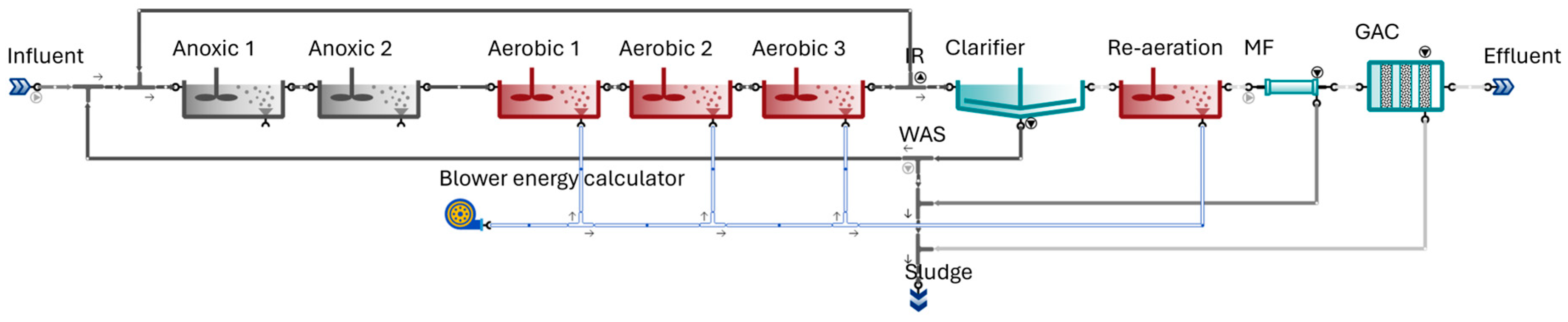
For the demonstration of BTEX modelling applications, a variant of the BSM1 test configuration [63] was set up in the Sumo22 simulation software and used to evaluate potential operational cost savings through controlling the sludge retention time or by air stripping and through comparing strategies of GAC tower maintenance. The chosen technological sequence is a simulation benchmark that defines a relatively simple standard water resource recovery facility with influent loads provided, aimed at evaluating system performance based on test procedures, according to a given set of evaluation criteria. The BSM1 plant comprises a five-compartment activated sludge reactor cascade, including two anoxic zones and three aerobic zones. This setup combines nitrification with pre-denitrification, a widely adopted arrangement for achieving biological nitrogen removal. Downstream of the reactor cascade, the configuration features a secondary clarifier for phase separation [63]. Table 1 summarizes the main characteristics of the benchmarking facility, regarding average dry weather conditions.
In addition to the BSM1 layout, Sumo22’s empirical blower and pump models were set up to assess energy and associated costs regarding aeration, return activated sludge pumping, nitrified mixed liquor recycle pumping as well as backwash pumping. Solving the rate expression and component balance equations of variables in wastewater treatment technologies requires a simulation environment based on biokinetics. From an operational strategic point of view, process modelling can reveal cost-down opportunities by experimenting with control strategies and pointing out necessary interventions for complying with environmental regulations. Sumo22 is a multipurpose, open-source environment that has been developed specifically for dynamic environmental modelling, with particular emphasis on municipal and industrial wastewater treatment plants. Sumo22 can simulate a wide variety of BNR (biological nutrient removal) plant configurations [30].
According to the model layout prepared for the study, portrayed by Figure 1, as a fictive retrofit of the municipal plant with effluent purification, the scope of the standard BSM1 configuration was extended with a granular activated carbon process and a microfiltration step prior to GAC for the sake of mechanical protection against the remaining solids overflowing from the secondary clarifiers. In the granular activated carbon unit process model, the replacement frequency of the exhausted bed is determined based on the TOC adsorption capacity of the media and the load of soluble organics removed. It can be run in either a quasi steady-state mode, where the AC demand is quantified from an instantaneous carbon mass balance, or in dynamic mode, where it is calculated cyclically, based on the effluent quality predicted using an empirical asymmetric breakthrough curve. The total bed volume of the towers was sized as 50 m3; with the effluent quality and quantity associated with the BSM1 use case, this ought to require bed replacement roughly every month, assuming that the bed density is 450 kg m−3 and that the soluble organic carbon adsorption capacity of the bed is 0.2 gC gAC−1, estimated based on operational expertise. The MF and GAC units are backwashed in half-hour and daily cycles, respectively, for industrial safety reasons against solids depositing on the filter and the granular media. We note here that bed replacement can be calculated automatically in Sumo22 from the mass flow of the BTEX compounds removed, simulating how—in a full-scale treatment plant—the operators would remove exhausted granules and reinstall fresh granules periodically, whenever the breakpoint of the media is reached. After sedimentation, an additional re-aeration zone with the hydraulic retention time of 0.3 h—with coarse bubble aeration—is used to maintain sufficient dissolved oxygen levels required for the effluent quality. The influent quality regarding BTEX concentrations was characterized according to typical levels in municipal wastewater, containing 303 µg L−1 of benzene, 290 µg L−1 of toluene, 249 µg L−1 of ethylbenzene and 933 µg L−1 of xylene [64].
Using the scenario analysis functionality of Sumo22, the targeted sludge retention time and the air flow to the re-aeration tanks were selected as the input parameters to be changed in between the simulation runs in order to efficiently evaluate the changes in the blower energy demand, the yearly requirement of GAC and the amount of BTEX chemicals removed. SRT control is handled according to the BSM1 scenario guidelines; Sumo22 automatically adjusts the wasted sludge flow rate, varying the activated sludge solids concentration to meet the SRT target.
3. Results and Discussion
The simulation and results interpretation involved preparing the model output setup for exporting variables linked to pollutant loads, composition profiles, effluent quality, biodegradation, stripping and adsorption rates as well as calculations on resources, regarding aeration requirement and activated carbon consumption. Sumo22’s combined global and local solvers were used to handle the integrated calculations necessary for plant-wide modelling. Based on a steady-state simulation featuring a BSM1 baseline scenario, Figure 2 displays a profile of the summed BTEX component uptake and stripping rates throughout the biological treatment, expressed in the mass flow of COD per reactor cell volume.
The BTEX biodegradation and stripping rate profiles represent the plug-flow characteristics of the treatment plant; degradation is most significant at the first anoxic cell because, here, the BTEX compounds serve as substrates for the biomass in the highest concentration. There is a decline in biological uptake in the second anoxic zone as substrate availability becomes more limited, but as the wastewater enters the first aerated compartment, the degradation rate is boosted due to the faster aerobic reactions. The elimination of BTEX compounds through gas exchange is mainly visible at aerobic zones due to the contribution of air stripping driving out greater mass flows of volatile contaminants; stripping from anoxic compartments is mostly limited to the interface of the liquid surface and the atmosphere. Throughout the aerated cells, the profiles of removal rates attributed to both biodegradation and stripping correspond well with the decreasing concentration gradient of BTEX pollutants during activated sludge treatment.
In this section on demonstrated studies, the analysis is primarily centered around examining the model concept in detail based on SRT, followed by an evaluation of the effect of air stripping and concluding with a presentation of GAC operational strategy modelling.
3.1. SRT-Based Scenarios
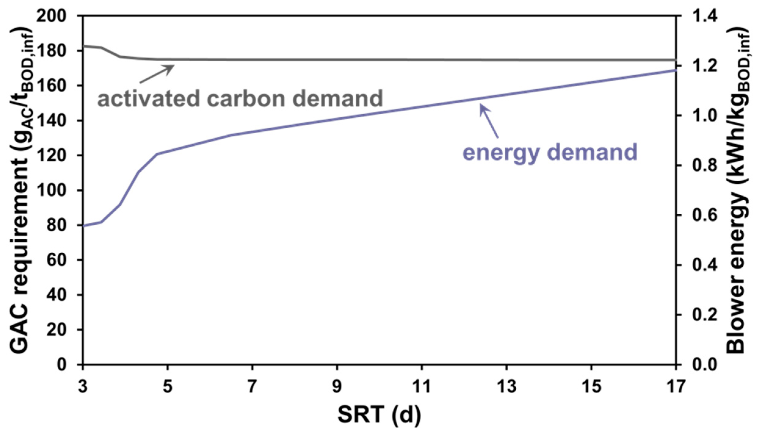
In the first modelling experiment, the test configuration ran at a steady state in dry weather conditions; using Sumo22’s combined global and local solvers, a series of runs were performed with varied SRT to obtain the blower power consumption and the required mass flow of the GAC bed to be replaced. From these variables and the raw influent characteristics regarding BSM1 specifications, the blower energy and activated carbon demand specific to the influent BOD were plotted, as shown in Figure 3, to provide more generic results irrespective of the benchmarking plant capacity.
The results show that the reduction in demand for the GAC replacement is most significant within the range of 3 to 6 days of SRT. However, this range would not be typical for a water reclamation plant, as even at warm/moderate water temperatures, longer retention times are needed for proper nutrient removal. It typically takes between 10 and 15 days for a thorough nitrification–denitrification process. If the SRT falls below this range, the process remains incomplete. Conversely, if the SRT exceeds this range, the plant’s energy efficiency is compromised [65]. After 6 days, the further decrease in the activated carbon demand is not significant, given that, proportionally, a much higher performance is demanded from the blowers to meet the dissolved oxygen concentration target at higher biomass concentrations. The reason behind this is that most of the organic load treated by the towers is of the soluble unbiodegradable organic fraction, the decomposition of which cannot be boosted by raising the sludge residence time.
Apart from the operating cost, another important aspect of micropollutant removal is the effluent quality. The BTEX concentrations in the treated water were also plotted against the same range of SRT, as displayed in Figure 4. The difference in BTEX removal is most significant between the SRT range of 3 to 6 days, as a greater load of contaminants, which were not exposed to the biomass for a sufficient amount of time to be treated, bleed through the GAC bed. Consequently, it is important to note that the activated sludge system must always be operated responsibly, not allowing the SRT to drop below the necessary level for nutrient removal, as the activated carbon treatment step might not adsorb the surplus in the load sufficiently to meet regulations, depending on the use case (e.g., reuse for agriculture, drinking water supply). Benstoem et al. [61] noted a decrease in micropollutant removal efficiency due to the improper functioning of a secondary clarifier, resulting in an increase in the average TSS concentration from 6 mg/L to a peak of 30 mg/L [66].
For interpreting the results of the modelling scenarios in more detail, the contributors to the BTEX metabolism throughout the treatment plant are shown in Figure 5, based on comparing the total mass flow of the compounds biodegraded, stripped and adsorbed to the influent BTEX load. The mass flows are interpreted in equivalent units of chemical oxygen demand. When discussing the COD percent removal of BTEX pollutants, according to the modelling study, biodegradation is predicted to be the most significant process—by raising the plant-wide SRT, a steep increase can be achieved in the extent of anoxic and anaerobic biodegradation. The increased biodegradation is in accordance with decreased stripping and the reduction in the adsorbed mass flows on the activated carbon beds since the remaining micropollutant load, to be removed by gas transfer or effluent polishing, drops.
However, as deduced from the results in Figure 4, most of the load fed to GAC treatment is in the form of soluble unbiodegradable compounds; therefore, there is only limited cost down capability in minimizing the bed replacement frequency through intensifying the activated sludge process. It can be concluded that, the more complete the nutrient removal is, the better the effluent quality is, including lower BTEX concentrations. However, the increased demand for aeration is more significant than the amount of activated carbon saved; thus, an actual SRT target is practically determined by how stringent the water quality requirements are. However, ultra-short SRT processes (<4 days) aiming for carbon removal from wastewater demonstrate high efficiency in organic matter separation and in enhancing energy recovery rates in wastewater treatment plants [67].
3.2. The Effect of Aeration Intensity
In another demonstrated case study of the developed numerical methods, the scenario analysis was conducted with varied aeration intensities of the facility’s post-aeration tanks for the different steady-state runs. The decision to modify air flow to this re-aeration process—rather than changing DO setpoints in the activated sludge trains—came down to the fact that oxygen transfer will be more effective in secondary clarifier effluent water than in mixed liquor due to the absence of biomass oxygen uptake and higher α factors. The volume to be aerated is also much smaller this way, with sufficient HRT for the reaction rate of stripping. Figure 6 presents these scenarios’ results on BOD-specific aeration energy and activated carbon demand as a function of superficial gas velocity—the air flow expressed per re-aeration tank surface area.
By raising the air supply to the post-aeration tanks, it was revealed that despite the less significant energy requirement increase compared to the trend seen through raising the SRT, it only provides negligible cost-saving opportunities in activated carbon usage.
The overall percent removal of BTEX chemicals is already quite high (99%), even with the lowest superficial gas velocity, and given that the majority of the organic load to be polished by GAC is not volatile and cannot be removed through air stripping, there is not much room for improvement by removing some of the remaining BTEX components. It must be noted that the water samples investigated in this paper are in the context of municipal wastewater treatment plants, with the inlet concentration of BTEX compounds being marginal compared to that of other pollutants that the technology focuses on removing. The proposal of the enhanced stripping of volatile pollutants from much more concentrated industrial wastewater, especially in the petroleum industry [68], to reduce the frequency of GAC bed replacement could make much more sense.
The impact of stripping enhancement on effluent BTEX concentrations is presented in Figure 7. It may be a viable method for stabilizing the effluent water quality regarding micropollutants through a relatively fast intervention. Regarding environmental security, emergencies in wastewater plants—such as operational difficulties with biological treatment—may cause a sudden load increase in BTEX contaminants fed to GAC columns, in which case online monitoring could alert operators to make a swift change in the air supply to the tanks prior to the adsorption process, preventing a violation of the tertiary treatment effluent water quality limits.
Figure 8 shows the removal percentage of the influent COD-based BTEX load through individual treatment mechanisms, as a function of the varied air flux. There is effectively no change in the contribution by biodegradation, since the re-aeration zone is located after the bioreactors, following the separation of biomass from the liquid phase by secondary clarification. Enhanced air stripping promotes the removal of the remaining BTEX constituents following biological treatment, whose concentrations are much smaller than those of the other remaining organic contaminants, therefore not being able to provide further minimization of the activated carbon requirement but potentially being useful for stabilizing water quality as a safe alternative to comply with effluent regulations. The fractional contribution of the adsorption process is inversely proportional to this trend. Figure 5 and Figure 8 emphasize that the developed plant-wide modelling tools also provide insight into variables that cannot be directly measured, which, in conclusion, can give engineers and operators a better process understanding. This is a useful feature of modelling tools that are calibrated and virtually linked to actual facilities in real time (e.g., through digital twin implementations) [69].
The authors stress that this paper focuses on the general implementation of a methodology for plant-wide process simulation involving the fate of BTEX pollutants in biological wastewater treatment, along with options of physico-chemical effluent polishing, and the experimental cases presented are for demonstrating the feasibility of the model applications in municipal wastewater treatment. Therefore, these results shall not be generalized to other sources of municipal wastewater and certainly not to industrial treatment. The verification of robustness and accuracy shall be performed as a future effort in modelling studies, not on a benchmarking tool but against measured data from existing facilities.
3.3. GAC Operational Strategies
A third modelling case featured dynamic runs to compare two different GAC operational strategies, as illustrated by Figure 9. Scheduling bed replacement on a fixed time interval basis may be beneficial for sustaining stable effluent quality; however, this is not a cost-effective option, as some useful carbon adsorption capacity is lost. The use of effluent monitoring (e.g., applying online TOC probes) to synchronize bed replacement with the breakthrough capacity of the bed, i.e., when a certain effluent concentration limit is reached, may enable a more than 15% operational cost reduction involving the GAC process.
Zietzschmann et al. (2016) [70] conducted small-scale tests with GAC to assess the adsorption of organic micropollutants (OMP) from sewage effluent. They observed that as long as influent concentrations remained below specific thresholds, the relative breakthrough behavior remained unaffected. Consequently, the capacity for OMP removal was directly correlated with the influent OMP concentration. However, the authors noted that using the specific throughput of dissolved organic carbon alone was insufficient to generate superimposed breakthrough curves [70]. In practice, when operating a full-scale facility, complete breakthrough curves shall never be able to be registered, as stable effluent quality must be maintained. We emphasize that the purpose of this research is not to generate accurate breakthrough curves but to provide a robust simulation of the breakpoint based on the adsorption capacity specification, thus aiding in decision-making about scheduling GAC bed replacement and the evaluation of operational and control strategies.
4. Conclusions
In this paper, the proposed kinetic concepts have been shown to provide a reasonable framework for simulating the fate of BTEX compounds in water resource recovery facilities. They can be merged with existing biokinetic models to be run in mathematical simulation software environments, as potential methods of effluent quality estimation and operational optimization in the areas of cost and resources.
The model-based benchmarking tests of this study demonstrated the applicability of the presented concepts for plant-wide modelling by investigating the impacts of operational parameters in the activated sludge process on the removal efficiency of BTEX chemicals, alongside the demand for granular activated carbon usage in effluent polishing. The first studied case revealed that the reduction in bed replacement frequency is most significant within the range of 3 to 6 days of SRT. Above 6 days, the further decrease in the AC requirement is less significant, and proportionally, a higher blower power is required to meet the DO setpoint at higher MLSS concentrations. Since BTEX constituents are only present at low concentrations in municipal settings, potential cost reductions in GAC bed replacement—through optimizing the biological treatment—may not be significant due to the higher fraction of inert and non-volatile material fed to GAC treatment, which cannot be removed through biodegradation and stripping, respectively. However, according to another studied example case, enhanced aeration for increased stripping prior to the GAC process may be a useful approach to preventing the deterioration of effluent quality regarding BTEX compounds in case of operational emergencies. The demonstration of dynamic simulation to compare operational strategies showed that synchronizing bed replacement with the activated carbon breakthrough capacity—based on the effluent quality—may result in more than 15% operational cost savings regarding the GAC process.
Goals for future studies include linking the model with further processes in water reuse. Efforts shall also be focused on model developments for off-gas treatment, considering the health risks—especially of benzene—in the atmosphere. Although the kinetic model parameters were set up based on values found in the scientific literature, future studies should aim for thorough model validation based on measured data from various facilities in municipal sewage treatment. As an outlook on degradation modelling with regard to granular activated carbon, future development efforts are dedicated to enhancing the GAC adsorption methodology with biomass activity included, enabling the simulation of BAC applications and lowered loading to an AC bed. The focus of potential further research could also be placed on applications in industrial wastewater treatment with a high BTEX content.
Author Contributions
Conceptualization, D.B. and T.K.; methodology, D.B., T.W. and F.H.; software, D.B., T.W. and F.H.; data curation, D.B., T.W. and F.H.; writing—original draft preparation, D.B. and T.K.; writing—review and editing, D.B. and T.K.; visualization, D.B.; supervision, T.K. All authors have read and agreed to the published version of the manuscript.
Funding
Project no. TKP2021-NVA-18 has been implemented with the support provided by the Ministry of Culture and Innovation of Hungary from the National Research, Development and Innovation Fund, financed under the TKP2021-NVA funding scheme.
Data Availability Statement
The data are contained within the article.
Conflicts of Interest
The authors declare no conflicts of interest.
Nomenclature
| α | alpha (wastewater/clean water) correction factor for mass transfer coefficient |
| abub | specific contact area between the gas bubble surface and liquid phase [m2 m−3] |
| asur | specific contact area between the surface gas and liquid phase [m2 m−3] |
| Adiff,sp | area per diffuser [m2] |
| Ar | liquid surface [m2] |
| β | beta (wastewater/clean water) correction factor for the saturation concentration |
| BTC | TOC breakthrough capacity (in concentration unit) [gC m−3] |
| BTCm | TOC adsorption capacity (at breakpoint, in mass fraction unit) [gC gAC−1] |
| Cmid | midpoint concentration of breakthrough curve, with asymmetry correction [gC m−3] |
| Cmid,symm | midpoint concentration of curve, without asymmetry correction [gC m−3] |
| coefflead,h,diff | leading coefficient in a diffuser submergence correction term [m−1] |
| coefflin,h,diff | linear coefficient in a diffuser submergence correction term [m−1] |
| dbub | bubble Sauter mean diameter [m] |
| ddiff | diffuser density [m2 m−2] |
| Di,25 | diffusion coefficient of gas state variable i in water [m2 d−1] |
| divd,diff | divisor value in a diffuser density correction term [m2 m−2] |
| ε | gas hold-up [m3gas m−3] |
| EQC,ad,total | carbon equivalent for all adsorbed components on a GAC bed [g C m−3] |
| expSSOTE | exponent in SSOTE correlation [d m−3gas] |
| F | diffuser fouling factor |
| Fac | replaced activated carbon mass flow [g d−1] |
| fcover | covered fraction of the reactor surface |
| FGi | mass flow of gas phase state variable i [g d−1] |
| fh,sat,eff | effective saturation depth fraction |
| fkL,i | fraction in the liquid side for the mass transfer of gas state variable i |
| FLi | mass flow of liquid phase state variable i [g d−1] |
| fwave | waviness factor |
| Gi | concentration of gas phase state variable i in off-gas, per liquid volume [g m−3] |
| Gi,air,inp | concentration of gas phase state variable i in the air input [%V V−1] |
| Gi,atm | concentration of gas phase state variable i in the atmosphere [%V V−1] |
| Gi,percent | concentration of gas phase state variable i in off-gas, percentage [%V V−1] |
| hdiff | diffuser submergence [m] |
| hdiff,floor | diffuser height from floor [m] |
| Henryi,dt | temperature dependency factor for Henry coefficient of gas i [K] |
| Henryi,SATP | Henry coefficient of gas i, standard (SATP) temperature (25 °C) [mol m−3 Pa−1] |
| hr | reactor depth [m] |
| hsat,eff | effective saturation depth [m] |
| hsea | elevation above sea level [m] |
| iC,i | equivalent mass of soluble organic state variable i per unit mass of carbon [g gC−1] |
| kL,i,bub,st,cw | liquid-side mass transfer coefficient for gas bubbles, standard conditions [m d−1] |
| kL,i,sur,st,cw | liquid-side mass transfer coefficient for liquid surface, standard conditions [m d−1] |
| kLai,bub | volumetric mass transfer coefficient for gas bubbles, field conditions [d−1] |
| kLai,bub,st,cw | volumetric mass transfer coefficient for gas bubbles, standard conditions [d−1] |
| kLai,sur | volumetric mass transfer coefficient for liquid surface, field conditions [d−1] |
| kLai,sur,st,cw | volumetric mass transfer coefficient for liquid surface, standard conditions [d−1] |
| Lair | temperature lapse rate for air pressure calculation [K m−1] |
| Li | concentration of liquid phase state variable i [g m−3] |
| Li,ad | adsorbed soluble organic state variable i mass per bed volume [g m−3] |
| Mac,cycle | mass of activated carbon filled per cycle [g] |
| magnmid,asymm | magnitude of the breakthrough curve midpoint asymmetry correction term |
| MMair | molar mass of air [g mol−1] |
| MMEQ,i | equivalent molar mass of gas phase state variable i [g mol−1] |
| ndiff | number of diffusers |
| ngas,bub | molar quantity of gas bubbles per unit liquid volume [mol m−3] |
| Nrepl | activated carbon bed replacement cycle frequency [d−1] |
| pair | air pressure at field elevation [Pa] |
| pgas | gas phase pressure [Pa] |
| pNTP | pressure at standard (NTP) conditions (101,325 Pa) [Pa] |
| powd,diff | power value in a diffuser density correction term |
| powh,diff | power value in a diffuser submergence correction term |
| powmid,asymm | power of the breakthrough curve midpoint asymmetry correction term |
| ppartial,i,bub | partial pressure of gas state variable i in the gas phase [Pa] |
| ppartial,i,bub,st | partial pressure of gas state variable i in the gas phase, standard conditions [Pa] |
| ppartial,i,sur | partial pressure of gas state variable i in the atmosphere [Pa] |
| ppartial,i,sur,st | partial pressure of gas state variable i in the atmosphere, standard conditions [Pa] |
| pst,h,sat,eff | pressure at standard conditions and effective saturation depth [Pa] |
| pv,T | saturated vapor pressure of water at temperature T [Pa] |
| θ | Arrhenius temperature correction factor for the mass transfer coefficient |
| Q | volumetric flow of wastewater [m3 d−1] |
| Qair,NTP | air flow at standard (NTP) conditions [m3gas d−1] |
| Qair,NTP,sp | air flow per diffuser at standard (NTP) conditions [m3gas d−1] |
| Qgas,transfer,NTP | gas transfer flow at standard (NTP) conditions [m3gas d−1] |
| Qgas,outp,NTP | off-gas flow at standard (NTP) conditions [m3gas d−1] |
| ρac | apparent density of granular activated carbon [gAC m−3] |
| rateFi | mass rate of state variable i [g d−1] |
| ratei | reaction rate for the state variable [g m−3 d−1] |
| RemGAC,i | removal ratio of soluble organic state variable i by granular activated carbon |
| rj | process rate regarding process j (from Gujer matrix) [g m−3 d−1] |
| Si,bub,sat | saturation concentration at the gas bubble interface [g m−3] |
| Si,bub,sat,st,cw | saturation concentration at the gas bubble interface, standard conditions [g m−3] |
| Si,sur,sat | saturation concentration at the atmospheric interface [g m−3] |
| Si,sur,sat,st,cw | saturation concentration at the atmospheric interface, standard conditions [g m−3] |
| slbreak | slope of the breakthrough curve [m3 gC−1] |
| SO2 | dissolved oxygen concentration [gO2 m−3] |
| SOTRbub | standard oxygen transfer rate from bubbles [g d−1] |
| SSOTE | specific standard oxygen transfer efficiency [% m−1] |
| SSOTE0 | intercept in SSOTE correlation [% m−1] |
| SSOTEasym | asymptote in SSOTE correlation [% m−1] |
| T | liquid temperature [°C] |
| Tair,K | field air temperature [K] |
| TK | liquid temperature in an SI unit [K] |
| TNTP,K | temperature at standard (NTP) conditions (20 °C) [K] |
| trepl | duration of activated carbon bed replacement [d] |
| TSATP,K | temperature at standard (SATP) conditions (25 °C) [K] |
| Vac | activated carbon bed volume [m3] |
| Vgas | gas phase volume [m3gas] |
| Vgas,NTP | gas phase volume at standard (NTP) conditions [m3gas] |
| vj,i | stoichiometric coefficient of state variable i in process j |
| Vr | reactive volume [m3] |
Appendix A. Gujer Matrix Development
The following tables show the MiniSumo biokinetic model structure, alongside BTEX-related model adjustments and the affected cells of the Gujer matrix based on reference [29]. All process rates are interpreted in gCOD m−3 d−1 units, with the exception of the elimination of surfactants, which is interpreted in d−1.

Table A1.
Gujer Matrix—part 1.
| Symbol | Process Name |
|---|---|
| 1 | OHO growth on VFAs, O2 |
| 2 | OHO growth on VFAs, NOx |
| 3 | OHO growth on benzene, O2 |
| 4 | OHO growth on benzene, NOx |
| 5 | OHO growth on toluene, O2 |
| 6 | OHO growth on toluene, NOx |
| 7 | OHO growth on ethylbenzene, O2 |
| 8 | OHO growth on ethylbenzene, NOx |
| 9 | OHO growth on xylene, O2 |
| 10 | OHO growth on xylene, NOx |
| 11 | OHO growth on SB, O2 |
| 12 | OHO growth on SB, NOx |
| 13 | SB fermentation with high VFA (OHO growth, anaerobic) |
| 14 | SB fermentation with low VFA (OHO growth, anaerobic) |
| 15 | Benzene fermentation with low VFA (OHO growth, anaerobic) |
| 16 | Toluene fermentation with low VFA (OHO growth, anaerobic) |
| 17 | Ethylbenzene fermentation with low VFA (OHO growth, anaerobic) |
| 18 | Xylene fermentation with low VFA (OHO growth, anaerobic) |
| 19 | OHO decay |
| 20 | NITO growth |
| 21 | NITO decay |
| 22 | AMETO growth |
| 23 | AMETO decay |
| 24 | HMETO growth |
| 25 | HMETO decay |
| 26 | XB hydrolysis |
| 27 | XB anaerobic hydrolysis (fermentation) |
| 28 | SN,B ammonification |
| 29 | NOx assimilative reduction |
| 30 | FeP precipitation |
| 31 | FeP redissolution |
| 32 | AlP precipitation |
| 33 | AlP redissolution |
| 34 | Elimination of surfactants |
| 35 | Methane gas transfer—bubbles |
| 36 | Hydrogen gas transfer—bubbles |
| 37 | Oxygen gas transfer—bubbles |
| 38 | Nitrogen gas transfer—bubbles |
| 39 | Benzene gas transfer—bubbles |
| 40 | Toluene gas transfer—bubbles |
| 41 | Ethylbenzene gas transfer—bubbles |
| 42 | Xylene gas transfer—bubbles |
| 43 | Methane gas transfer—surface |
| 44 | Hydrogen gas transfer—surface |
| 45 | Oxygen gas transfer—surface |
| 46 | Nitrogen gas transfer—surface |
| 47 | Benzene gas transfer—surface |
| 48 | Toluene gas transfer—surface |
| 49 | Ethylbenzene gas transfer—surface |
| 50 | Xylene gas transfer—surface |
Table A2.
Gujer Matrix—part 2.
| SBENE | STENE | SEBENE | SXENE | SB | XB | SU | XU | XE | XOHO | |
|---|---|---|---|---|---|---|---|---|---|---|
| 1 | 1 | |||||||||
| 2 | 1 | |||||||||
| 3 | −1/YOHO,BTEX,ox | 1 | ||||||||
| 4 | −1/YOHO,BTEX,anox | 1 | ||||||||
| 5 | −1/YOHO,BTEX,ox | 1 | ||||||||
| 6 | −1/YOHO,BTEX,anox | 1 | ||||||||
| 7 | −1/YOHO,BTEX,ox | 1 | ||||||||
| 8 | −1/YOHO,BTEX,anox | 1 | ||||||||
| 9 | −1/YOHO,BTEX,ox | 1 | ||||||||
| 10 | −1/YOHO,BTEX,anox | 1 | ||||||||
| 11 | −1/YOHO,SB,ox | 1 | ||||||||
| 12 | −1/YOHO,SB,anox | 1 | ||||||||
| 13 | −1/YOHO,SB,ana | 1 | ||||||||
| 14 | −1/YOHO,SB,ana | 1 | ||||||||
| 15 | −1/YOHO,BTEX,ana | 1 | ||||||||
| 16 | −1/YOHO,BTEX,ana | 1 | ||||||||
| 17 | −1/YOHO,BTEX,ana | 1 | ||||||||
| 18 | −1/YOHO,BTEX,ana | 1 | ||||||||
| 19 | 1 − fE | fE | −1 | |||||||
| 21 | 1 − fE | fE | ||||||||
| 23 | 1 − fE | fE | ||||||||
| 25 | 1 − fE | fE | ||||||||
| 26 | 1 | −1 | ||||||||
| 27 | 1 − fH2 | −1 | ||||||||
| 29 | −EEQNO3 × XOHO/XBIO,kin | |||||||||
| 39 | 1 | |||||||||
| 40 | 1 | |||||||||
| 41 | 1 | |||||||||
| 42 | 1 | |||||||||
| 47 | 1 | |||||||||
| 48 | 1 | |||||||||
| 49 | 1 | |||||||||
| 50 | 1 |
Table A3.
Gujer Matrix—part 3.
| SVFA | |
|---|---|
| 1 | −1/YOHO,VFA,ox |
| 2 | −1/YOHO,VFA,anox |
| 13 | (1 − YOHO,SB,ana − YOHO,H2,ana,high)/YOHO,SB,ana |
| 14 | (1 − YOHO,SB,ana − YOHO,H2,ana,low)/YOHO,SB,ana |
| 15 | (1 − YOHO,SB,ana − YOHO,H2,ana,low)/YOHO,SB,ana |
| 16 | (1 − YOHO,SB,ana − YOHO,H2,ana,low)/YOHO,SB,ana |
| 17 | (1 − YOHO,SB,ana − YOHO,H2,ana,low)/YOHO,SB,ana |
| 18 | (1 − YOHO,SB,ana − YOHO,H2,ana,low)/YOHO,SB,ana |
| 22 | −1/YAMETO |
Table A4.
Gujer Matrix—part 4.
| XNITO | XAMETO | XHMETO | |
|---|---|---|---|
| 20 | 1 | ||
| 21 | −1 | ||
| 22 | 1 | ||
| 23 | −1 | ||
| 24 | 1 | ||
| 25 | −1 | ||
| 29 | −EEQNO3 × XNITO/XBIO,kin | −EEQNO3 × XAMETO/XBIO,kin | −EEQNO3 × XHMETO/XBIO,kin |
Table A5.
Gujer Matrix—part 5.
| SNHx | SNOx | SN2 | |
|---|---|---|---|
| 1 | −iN,BIO | ||
| 2 | −iN,BIO | −(1 − YOHO,VFA,anox)/(EEQN2,NO3 × YOHO,VFA,anox) | (1 − YOHO,VFA,anox)/(EEQN2,NO3 × YOHO,VFA,anox) |
| 3 | −iN,BIO | ||
| 4 | −iN,BIO | −(1 − YOHO,BTEX,anox)/(EEQN2,NO3 × YOHO,BTEX,anox) | (1 − YOHO,BTEX,anox)/(EEQN2,NO3 × YOHO,BTEX,anox) |
| 5 | −iN,BIO | ||
| 6 | −iN,BIO | −(1 − YOHO,BTEX,anox)/(EEQN2,NO3 × YOHO,BTEX,anox) | (1 − YOHO,BTEX,anox)/(EEQN2,NO3 × YOHO,BTEX,anox) |
| 7 | −iN,BIO | ||
| 8 | −iN,BIO | −(1 − YOHO,BTEX,anox)/(EEQN2,NO3 × YOHO,BTEX,anox) | (1 − YOHO,BTEX,anox)/(EEQN2,NO3 × YOHO,BTEX,anox) |
| 9 | −iN,BIO | ||
| 10 | −iN,BIO | −(1 − YOHO,BTEX,anox)/(EEQN2,NO3 × YOHO,BTEX,anox) | (1 − YOHO,BTEX,anox)/(EEQN2,NO3 × YOHO,BTEX,anox) |
| 11 | −iN,BIO | ||
| 12 | −iN,BIO | −(1 − YOHO,SB,anox)/(EEQN2,NO3 × YOHO,SB,anox) | (1 − YOHO,SB,anox)/(EEQN2,NO3 × YOHO,SB,anox) |
| 13 | −iN,BIO | ||
| 14 | −iN,BIO | ||
| 15 | −iN,BIO | ||
| 16 | −iN,BIO | ||
| 17 | −iN,BIO | ||
| 18 | −iN,BIO | ||
| 19 | −fE × (iN,XE − iN,BIO) | ||
| 20 | −1/YNITO − iN,BIO | 1/YNITO | |
| 21 | −fE × (iN,XE − iN,BIO) | ||
| 22 | −iN,BIO | ||
| 23 | −fE × (iN,XE − iN,BIO) | ||
| 24 | −iN,BIO | ||
| 25 | −fE × (iN,XE − iN,BIO) | ||
| 28 | 1 | ||
| 29 | 1 + EEQNO3 × iN,BIO | −1 | |
| 38 | 1 | ||
| 46 | 1 |
Table A6.
Gujer Matrix—part 6.
| SN,B | XN,B | SPO4 | XP,B | SO2 | SCH4 | SH2 | |
|---|---|---|---|---|---|---|---|
| 1 | −iP,BIO | −(1 − YOHO,VFA,ox)/YOHO,VFA,ox | |||||
| 2 | −iP,BIO | ||||||
| 3 | −iP,BIO | −(1 − YOHO,BTEX,ox)/YOHO,BTEX,ox | |||||
| 4 | −iP,BIO | ||||||
| 5 | −iP,BIO | −(1 − YOHO,BTEX,ox)/YOHO,BTEX,ox | |||||
| 6 | −iP,BIO | ||||||
| 7 | −iP,BIO | −(1 − YOHO,BTEX,ox)/YOHO,BTEX,ox | |||||
| 8 | −iP,BIO | ||||||
| 9 | −iP,BIO | −(1 − YOHO,BTEX,ox)/YOHO,BTEX,ox | |||||
| 10 | −iP,BIO | ||||||
| 11 | −iP,BIO | −(1 − YOHO,SB,ox)/YOHO,SB,ox | |||||
| 12 | −iP,BIO | ||||||
| 13 | −iP,BIO | YOHO,H2,ana,high/YOHO,SB,ana | |||||
| 14 | −iP,BIO | YOHO,H2,ana,low/YOHO,SB,ana | |||||
| 15 | −iP,BIO | YOHO,H2,ana,low/YOHO,BTEX,ana | |||||
| 16 | −iP,BIO | YOHO,H2,ana,low/YOHO,BTEX,ana | |||||
| 17 | −iP,BIO | YOHO,H2,ana,low/YOHO,BTEX,ana | |||||
| 18 | −iP,BIO | YOHO,H2,ana,low/YOHO,BTEX,ana | |||||
| 19 | (1 − fE) × iN,BIO | (1 − fE) × iP,BIO | |||||
| 20 | −iP,BIO | −(EEQNO3 − YNITO)/YNITO | |||||
| 21 | (1 − fE) × iN,BIO | (1 − fE) × iP,BIO | |||||
| 22 | −iP,BIO | (1 − YAMETO)/YAMETO | |||||
| 23 | (1 − fE) × iN,BIO | (1 − fE) × iP,BIO | |||||
| 24 | −iP,BIO | (1 − YHMETO)/YHMETO | −1/YHMETO | ||||
| 25 | (1 − fE) × iN,BIO | (1 − fE) × iP,BIO | |||||
| 26 | XN,B/XB | −XN,B/XB | XP,B/XB | −XP,B/XB | |||
| 27 | XN,B/XB | −XN,B/XB | XP,B/XB | −XP,B/XB | fH2 | ||
| 28 | −1 | ||||||
| 29 | EEQNO3 × iP,BIO | ||||||
| 30 | −fP,Fe | ||||||
| 31 | fP,Fe | ||||||
| 32 | −fP,Al | ||||||
| 33 | fP,Al | ||||||
| 35 | 1 | ||||||
| 36 | 1 | ||||||
| 37 | 1 | ||||||
| 43 | 1 | ||||||
| 44 | 1 | ||||||
| 45 | 1 |
Table A7.
Gujer Matrix—part 7.
| SALK | XFeOH | XFeP | XAlOH | XAlP | |
|---|---|---|---|---|---|
| 1 | (−iN,BIO × CHNHx − iP,BIO × CHPO4) | ||||
| 2 | (−(1 − YOHO,VFA,anox)/(EEQN2,NO3 × YOHO,VFA,anox) × CHNO3 − iN,BIO × CHNHx − iP,BIO × CHPO4) | ||||
| 3 | (−iN,BIO × CHNHx − iP,BIO × CHPO4) | ||||
| 4 | (−(1 − YOHO,BTEX,anox)/(EEQN2,NO3 × YOHO,BTEX,anox) × CHNO3 − iN,BIO × CHNHx − iP,BIO × CHPO4) | ||||
| 5 | (−iN,BIO × CHNHx − iP,BIO × CHPO4) | ||||
| 6 | (−(1 − YOHO,BTEX,anox)/(EEQN2,NO3 × YOHO,BTEX,anox) × CHNO3 − iN,BIO × CHNHx − iP,BIO × CHPO4) | ||||
| 7 | (−iN,BIO × CHNHx − iP,BIO × CHPO4) | ||||
| 8 | (−(1 − YOHO,BTEX,anox)/(EEQN2,NO3 × YOHO,BTEX,anox) × CHNO3 − iN,BIO × CHNHx − iP,BIO × CHPO4) | ||||
| 9 | (−iN,BIO × CHNHx − iP,BIO × CHPO4) | ||||
| 10 | (−(1 − YOHO,BTEX,anox)/(EEQN2,NO3 × YOHO,BTEX,anox) × CHNO3 − iN,BIO × CHNHx − iP,BIO × CHPO4) | ||||
| 11 | (−iN,BIO × CHNHx − iP,BIO × CHPO4) | ||||
| 12 | (−(1 − YOHO,SB,anox)/(EEQN2,NO3 × YOHO,SB,anox) × CHNO3 − iN,BIO × CHNHx − iP,BIO × CHPO4) | ||||
| 13 | (−iN,BIO × CHNHx − iP,BIO × CHPO4) | ||||
| 14 | (−iN,BIO × CHNHx − iP,BIO × CHPO4) | ||||
| 15 | (−iN,BIO × CHNHx − iP,BIO × CHPO4) | ||||
| 16 | (−iN,BIO × CHNHx − iP,BIO × CHPO4) | ||||
| 17 | (−iN,BIO × CHNHx − iP,BIO × CHPO4) | ||||
| 18 | (−iN,BIO × CHNHx − iP,BIO × CHPO4) | ||||
| 19 | −fE × (iN,XE − iN,BIO) × CHNHx | ||||
| 20 | ((−1/YNITO − iN,BIO) × CHNHx + 1/YNITO × CHNO3 − iP,BIO × CHPO4) | ||||
| 21 | −fE × (iN,XE − iN,BIO) × CHNHx | ||||
| 22 | (−iN,BIO × CHNHx − iP,BIO × CHPO4) | ||||
| 23 | −fE × (iN,XE − iN,BIO) × CHNHx | ||||
| 24 | (−iN,BIO × CHNHx − iP,BIO × CHPO4) | ||||
| 25 | −fE × (iN,XE − iN,BIO) × CHNHx | ||||
| 26 | XP,B/XB × CHPO4 | ||||
| 27 | XP,B/XB × CHPO4 | ||||
| 28 | CHNHx | ||||
| 29 | ((1 + EEQNO3 × iN,BIO) × CHNHx − CHNO3 + EEQNO3 × iP,BIO × CHPO4) | ||||
| 30 | −fP,Fe × CHPO4 | −1 | 1 | ||
| 31 | fP,Fe × CHPO4 | 1 | −1 | ||
| 32 | −fP,Al × CHPO4 | −1 | 1 | ||
| 33 | fP,Al × CHPO4 | 1 | −1 |
Table A8.
Gujer Matrix—part 8.
| SALPHA | GCH4 | GH2 | GO2 | GN2 | GBENE | GTENE | GEBENE | GXENE | |
|---|---|---|---|---|---|---|---|---|---|
| 34 | 1 | ||||||||
| 35 | −1 | ||||||||
| 36 | −1 | ||||||||
| 37 | −1 | ||||||||
| 38 | −1 | ||||||||
| 39 | −1 | ||||||||
| 40 | −1 | ||||||||
| 41 | −1 | ||||||||
| 42 | −1 |
Table A9.
Gujer Matrix—part 9.
| Rate | |
|---|---|
| 1 | µOHO,T × XOHO × MsatSVFA,KVFA × MsatSO2,KO2,OHO × MsatSNHx,KNHx,BIO × MsatSPO4,KPO4,BIO × MsatSALK,KALK |
| 2 | µOHO,T × XOHO × ηOHO,anox × MsatSVFA,KVFA × MsatSNOx,KNOx,OHO × MinhSO2,KO2,OHO × MsatSNHx,KNHx,BIO × MsatSPO4,KPO4,BIO × MsatSALK,KALK |
| 3 | µOHO,BENE,T × XOHO × MsatSBENE,KBENE × MsatSO2,KO2,OHO × MsatSNHx,KNHx,BIO × MsatSPO4,KPO4,BIO × MsatSALK,KALK |
| 4 | µOHO,BENE,T × XOHO × ηOHO,anox × MsatSBENE,KBENE × MsatSNOx,KNOx,OHO × MinhSO2,KO2,OHO × MsatSNHx,KNHx,BIO × MsatSPO4,KPO4,BIO × MsatSALK,KALK |
| 5 | µOHO,TENE,T × XOHO × MsatSTENE,KTENE × MsatSO2,KO2,OHO × MsatSNHx,KNHx,BIO × MsatSPO4,KPO4,BIO × MsatSALK,KALK |
| 6 | µOHO,TENE,T × XOHO × ηOHO,anox × MsatSTENE,KTENE × MsatSNOx,KNOx,OHO × MinhSO2,KO2,OHO × MsatSNHx,KNHx,BIO × MsatSPO4,KPO4,BIO × MsatSALK,KALK |
| 7 | µOHO,EBENE,T × XOHO × MsatSEBENE,KEBENE × MsatSO2,KO2,OHO × MsatSNHx,KNHx,BIO × MsatSPO4,KPO4,BIO × MsatSALK,KALK |
| 8 | µOHO,EBENE,T × XOHO × ηOHO,anox × MsatSEBENE,KEBENE × MsatSNOx,KNOx,OHO × MinhSO2,KO2,OHO × MsatSNHx,KNHx,BIO × MsatSPO4,KPO4,BIO × MsatSALK,KALK |
| 9 | µOHO,XENE,T × XOHO × MsatSXENE,KXENE × MsatSO2,KO2,OHO × MsatSNHx,KNHx,BIO × MsatSPO4,KPO4,BIO × MsatSALK,KALK |
| 10 | µOHO,XENE,T × XOHO × ηOHO,anox × MsatSXENE,KXENE × MsatSNOx,KNOx,OHO × MinhSO2,KO2,OHO × MsatSNHx,KNHx,BIO × MsatSPO4,KPO4,BIO × MsatSALK,KALK |
| 11 | µOHO,T × MsatSB,KSB × MinhSVFA,KVFA × XOHO × MsatSO2,KO2,OHO × MsatSNHx,KNHx,BIO × MsatSPO4,KPO4,BIO × MsatSALK,KALK |
| 12 | µOHO,T × ηOHO,anox × MsatSB,KSB × MinhSVFA,KVFA × XOHO × MsatSNOx,KNOx,OHO × MinhSO2,KO2,OHO × MsatSNHx,KNHx,BIO × MsatSPO4,KPO4,BIO |
| 13 | µFERM,OHO,T × XOHO × LogsatSVFA,KVFA,FERM × MsatSB,KSB,ana × MinhSO2,KO2,OHO × MinhSNOx,KNOx,OHO × MsatSNHx,KNHx,BIO × MsatSPO4,KPO4,BIO × MsatSALK,KALK |
| 14 | µFERM,OHO,T × XOHO × LoginhSVFA,KVFA,FERM × MsatSB,KSB,ana × MinhSO2,KO2,OHO × MinhSNOx,KNOx,OHO × MsatSNHx,KNHx,BIO × MsatSPO4,KPO4,BIO × MsatSALK,KALK |
| 15 | µFERM,OHO,BENE,T × XOHO × LoginhSVFA,KVFA,FERM × MsatSBENE,KBENE,ana × MinhSO2,KO2,OHO × MinhSNOx,KNOx,OHO × MsatSNHx,KNHx,BIO × MsatSPO4,KPO4,BIO × MsatSALK,KALK |
| 16 | µFERM,OHO,TENE,T × XOHO × LoginhSVFA,KVFA,FERM × MsatSTENE,KTENE,ana × MinhSO2,KO2,OHO × MinhSNOx,KNOx,OHO × MsatSNHx,KNHx,BIO × MsatSPO4,KPO4,BIO × MsatSALK,KALK |
| 17 | µFERM,OHO,EBENE,T × XOHO × LoginhSVFA,KVFA,FERM × MsatSEBENE,KEBENE,ana × MinhSO2,KO2,OHO × MinhSNOx,KNOx,OHO × MsatSNHx,KNHx,BIO × MsatSPO4,KPO4,BIO × MsatSALK,KALK |
| 18 | µFERM,OHO,XENE,T × XOHO × LoginhSVFA,KVFA,FERM × MsatSXENE,KXENE,ana × MinhSO2,KO2,OHO × MinhSNOx,KNOx,OHO × MsatSNHx,KNHx,BIO × MsatSPO4,KPO4,BIO × MsatSALK,KALK |
| 19 | bOHO,T × XOHO × (MsatSO2,KO2,OHO + ηb,anox × MsatSNOx,KNOx,OHO × MinhSO2,KO2,OHO + ηb,ana × MinhSNOx,KNOx,OHO × MinhSO2,KO2,OHO) |
| 20 | µNITO,T × MsatSNHx,KNHx,NITO × XNITO × MsatSO2,KO2,NITO × MsatSPO4,KPO4,BIO × MsatSALK,KALK |
| 21 | bNITO,T × XNITO × (MsatSO2,KO2,NITO + ηb,anox × MsatSNOx,KNOx,NITO × MinhSO2,KO2,NITO + ηb,ana × MinhSNOx,KNOx,NITO × MinhSO2,KO2,NITO + mtox,ana) |
| 22 | µAMETO,T × HsatSVFA,AMETO × XAMETO × MinhSO2,KiO2,AMETO × MinhSNOx,KNOx,AMETO × MsatSNHx,KNHx,BIO × MsatSPO4,KPO4,BIO × MsatSALK,KALK |
| 23 | bAMETO,T × XAMETO × (MsatSO2,KiO2,AMETO + ηb,anox × MsatSNOx,KNOx,AMETO × MinhSO2,KiO2,AMETO + ηb,ana × MinhSNOx,KNOx,AMETO × MinhSO2,KiO2,AMETO) |
| 24 | µHMETO,T × MsatSH2,KH2,HMETO × XHMETO × MinhSO2,KiO2,HMETO × MinhSNOx,KNOx,HMETO × MsatSNHx,KNHx,BIO × MsatSPO4,KPO4,BIO × MsatSALK,KALK |
| 25 | bHMETO,T × XHMETO × (MsatSO2,KiO2,HMETO + ηb,anox × MsatSNOx,KNOx,HMETO × MinhSO2,KiO2,HMETO + ηb,ana × MinhSNOx,KNOx,HMETO × MinhSO2,KiO2,HMETO) |
| 26 | qHYD,T × XBIO,kin × MRsatXB,XBIO,kin,KHYD × (MsatSO2,KO2,OHO + ηb,anox × MsatSNOx,KNOx,OHO × MinhSO2,KO2,OHO) × MsatSALK,KALK |
| 27 | qHYD,T × XBIO,kin × MRsatXB,XBIO,kin,KHYD × ηb,ana × MinhSNOx,KNOx,OHO × MinhSO2,KO2,OHO × MsatSALK,KALK |
| 28 | qAMMON,T × SN,B × XBIO,kin |
| 29 | qASSIM,T × MsatSNOx,KNOx,ASSIM × MinhSNHx,KiNHx,ASSIM × XBIO,kin |
| 30 | qFeOH,PREC,Me × SPO4 × XFeOH |
| 31 | qFeOH,DISSOL,Me × XFeP × MsatSALK,KALK |
| 32 | qAlOH,PREC,Me × SPO4 × XAlOH |
| 33 | qAlOH,DISSOL,Me × XAlP × MsatSALK,KALK |
| 34 | qALPHA,O2 × XVSS × dampALPHA × (SALPHA,sat — SALPHA) |
| 35 | kLaGCH4,bub × (SGCH4,bub,sat — SCH4) |
| 36 | kLaGH2,bub × (SGH2,bub,sat — SH2) |
| 37 | kLaGO2,bub × (SGO2,bub,sat — SO2) |
| 38 | kLaGN2,bub × (SGN2,bub,sat — SN2) |
| 39 | kLaGBENE,bub × (SGBENE,bub,sat — SBENE) |
| 40 | kLaGTENE,bub × (SGTENE,bub,sat — STENE) |
| 41 | kLaGEBENE,bub × (SGEBENE,bub,sat — SEBENE) |
| 42 | kLaGXENE,bub × (SGXENE,bub,sat — SXENE) |
| 43 | kLaGCH4,sur × (SGCH4,sur,sat — SCH4) |
| 44 | kLaGH2,sur × (SGH2,sur,sat — SH2) |
| 45 | kLaGO2,sur × (SGO2,sur,sat — SO2) |
| 46 | kLaGN2,sur × (SGN2,sur,sat — SN2) |
| 47 | kLaGBENE,sur × (SGBENE,sur,sat — SBENE) |
| 48 | kLaGTENE,sur × (SGTENE,sur,sat — STENE) |
| 49 | kLaGEBENE,sur × (SGEBENE,sur,sat — SEBENE) |
| 50 | kLaGXENE,sur × (SGXENE,sur,sat — SXENE) |
where the following functions were used:
Table A10.
Nomenclature of the functions used in Gujer Matrix.
| Symbol | Name | Expression |
|---|---|---|
| Msat(var; k) | Monod saturation | var/(k + var) |
| Minh(var; k) | Monod inhibition | k/(k + var) |
| MRsat(s;x;k) | Monod ratio saturation | (s/x)/(s/x + k) |
| Logsat(var; halfval; slope) | Logistic saturation | 1/(1 + Exp((halfval − var) × slope)) |
| Loginh(var; halfval; slope) | Logistic inhibition | 1/(1 + Exp((var − halfval) × slope)) |
| Hsat(var; halfval; halfinh) | Haldane equation | var/(halfval + var + (var2/halfinh)) |
Appendix B. BTEX Kinetic and Stoichiometric Model Parameters
The following tables only show the BTEX-related model parameters introduced in this study. For a complete list of parameters, please refer to the MiniSumo process model.
Table A11.
BTEX kinetic and Stoichiometric Model Parameters.
| Ordinary Heterotrophic Organism Kinetics (OHO) | |||
|---|---|---|---|
| Symbol | Name | Value | Unit |
| µOHO,BENE | Maximum specific growth rate of OHOs on benzene | 0.006 | d−1 |
| µOHO,TENE | Maximum specific growth rate of OHOs on toluene | 0.014 | d−1 |
| µOHO,EBENE | Maximum specific growth rate of OHOs on ethylbenzene | 0.014 | d−1 |
| µOHO,XENE | Maximum specific growth rate of OHOs on xylene | 0.010 | d−1 |
| µFERM,OHO,BENE | Fermentation growth rate of OHOs on benzene | 0.0030 | d−1 |
| µFERM,OHO,TENE | Fermentation growth rate of OHOs on toluene | 0.0042 | d−1 |
| µFERM,OHO,EBENE | Fermentation growth rate of OHOs on ethylbenzene | 0.0035 | d−1 |
| µFERM,OHO,XENE | Fermentation growth rate of OHOs on xylene | 0.0050 | d−1 |
| KBENE | Half-saturation of benzene for OHOs | 6.8 | gCOD m−3 |
| KTENE | Half-saturation of toluene for OHOs | 14.8 | gCOD m−3 |
| KEBENE | Half-saturation of ethylbenzene for OHOs | 3.8 | gCOD m−3 |
| KXENE | Half-saturation of xylene for OHOs | 17.6 | gCOD m−3 |
| KBENE,ana | Half-saturation of benzene in fermentation by OHOs | 238 | gCOD m−3 |
| KTENE,ana | Half-saturation of toluene in fermentation by OHOs | 310 | gCOD m−3 |
| KEBENE,ana | Half-saturation of ethylbenzene in fermentation by OHOs | 67 | gCOD m−3 |
| KXENE,ana | Half-saturation of xylene in fermentation by OHOs | 615 | gCOD m−3 |
| Stoichiometric yields | |||
| Symbol | Name | Value | Unit |
| YOHO,BTEX,ox | Yield of OHOs on BTEX under aerobic conditions | 0.55 | g XOHO g SBTEX−1 |
| YOHO,BTEX,anox | Yield of OHOs on BTEX under anoxic conditions | 0.35 | g XOHO g SBTEX−1 |
| YOHO,BTEX,ana | Yield of OHOs on BTEX under anaerobic conditions | 0.10 | g XOHO g SBTEX−1 |
Appendix C. Gas Transfer, Aeration and BTEX Model Parameters
Table A12.
Gas Transfer, Aeration and BTEX Model Parameters.
| Henry Coefficients | |||
|---|---|---|---|
| Symbol | Name | Value | Unit |
| HenryBENE,25 | Henry coefficient for benzene at 25 °C | 1.70 × 10⁻³ | mol m−3 Pa−1 |
| HenryBENE,dt | Henry’s law temperature dependency factor of benzene | 4150 | K |
| HenryTENE,25 | Henry coefficient for toluene at 25 °C | 1.50 × 10⁻³ | mol m−3 Pa−1 |
| HenryTENE,dt | Henry’s law temperature dependency factor of toluene | 4150 | K |
| HenryEBENE,25 | Henry coefficient for ethylbenzene at 25 °C | 1.27 × 10⁻³ | mol m−3 Pa−1 |
| HenryEBENE,dt | Henry’s law temperature dependency factor of ethylbenzene | 5100 | K |
| HenryXENE,25 | Henry coefficient for xylene at 25 °C | 1.56 × 10⁻³ | mol m−3 Pa−1 |
| HenryXENE,dt | Henry’s law temperature dependency factor of xylene | 4083 | K |
| Diffusion coefficients | |||
| Symbol | Name | Value | Unit |
| DBENE,25 | Diffusion coefficient of benzene in water at 25 °C | 9.13 × 10⁻⁵ | m2 d−1 |
| DTENE,25 | Diffusion coefficient of toluene in water at 25 °C | 7.89 × 10⁻⁵ | m2 d−1 |
| DEBENE,25 | Diffusion coefficient of ethylbenzene in water at 25 °C | 7.27 × 10⁻⁵ | m2 d−1 |
| DXENE,25 | Diffusion coefficient of xylene in water at 25 °C | 7.08 × 10⁻⁵ | m2 d−1 |
| Oxygen transfer efficiency correlation parameters | |||
| Symbol | Name | Value | Unit |
| SSOTE0 | Intercept in SSOTE correlation | 7.77 | % m−1 |
| expSSOTE | Exponent (absolute value) in SSOTE correlation | 0.01041 | d m−3gas |
| SSOTEasym | Asymptote in SSOTE correlation | 5.75 | % m−1 |
| divd,diff | Divisor value in a diffuser density correction term | 0.1173 | m2 m−2 |
| powd,diff | Power value in a diffuser density correction term | 0.1329 | |
| coefflead,h,diff | Leading coefficient in a diffuser submergence correction term | 0.011 | m−1 |
| powh,diff | Power value in a diffuser submergence correction term | 1.6031 | |
| coefflin,h,diff | Linear coefficient in a diffuser submergence correction term | −0.0229 | m−1 |
| Specific molecular masses | |||
| Symbol | Name | Value | Unit |
| MMEQ,GBENE | Equivalent molar mass of benzene | 239.97 | gCOD mol−1 |
| MMEQ,GTENE | Equivalent molar mass of toluene | 287.96 | gCOD mol−1 |
| MMEQ,GEBENE | Equivalent molar mass of ethylbenzene | 335.95 | gCOD mol−1 |
| MMEQ,GXENE | Equivalent molar mass of xylene | 335.95 | gCOD mol−1 |
Appendix D. GAC Model Parameters
Table A13.
GAC Model Parameters.
| State Variable Equivalent Mass Ratios to Carbon | |||
|---|---|---|---|
| Symbol | Name | Value | Unit |
| iC,VFA | COD-to-carbon-mass ratio of VFA | 5.33 | gCOD gC−1 |
| iC,BENE | COD-to-carbon-mass ratio of benzene | 19.98 | gCOD gC−1 |
| iC,TENE | COD-to-carbon-mass ratio of toluene | 23.98 | gCOD gC−1 |
| iC,EBENE | COD-to-carbon-mass ratio of ethylbenzene | 27.97 | gCOD gC−1 |
| iC,XENE | COD-to-carbon-mass ratio of xylene | 27.97 | gCOD gC−1 |
| iC,SB | COD-to-carbon-mass ratio of readily biodegradable substrate | 3.20 | gCOD gC−1 |
| iC,SU | COD-to-carbon-mass ratio of soluble unbiodegradable organics | 2.80 | gCOD gC−1 |
| iC,SN,B | Nitrogen-to-carbon-mass ratio of soluble biodegradable organic N | 1.17 | gN gC−1 |
| Breakthrough curve parameters | |||
| Symbol | Name | Value | Unit |
| fbreak | Breakpoint fraction | 0.05 | |
| slbreak | Breakthrough curve slope | 0.00015 | m3 g−1 |
| powmid,asymm | Power of the midpoint asymmetry correction term | 20.00 | |
| magnmid,asymm | Magnitude of the midpoint asymmetry correction term | 0.50 | |
References
- Scheierling, S.M.; Bartone, C.; Mara, D.D.; Drechsel, P. Improving Wastewater Use in Agriculture: An Emerging Priority; World Bank Policy Research Working Paper Series 5412; The World Bank: Washington, DC, USA, 2010. [Google Scholar] [CrossRef]
- Scheierling, S.M.; Bartone, C.R.; Mara, D.D.; Drechsel, P. Towards an agenda for improving wastewater use in agriculture. Water Int. 2011, 36, 420–440. [Google Scholar] [CrossRef]
- Ofori, S.; Puškáčová, A.; Růžičková, I.; Wanner, J. Treated wastewater reuse for irrigation: Pros and cons. Sci. Total Environ. 2021, 760, 144026. [Google Scholar] [CrossRef] [PubMed]
- Pedrero, F.; Kalavrouziotis, I.; Alarcón, J.J.; Koukoulakis, P.; Asano, T. Use of treated municipal wastewater in irrigated agriculture—Review of some practices in Spain and Greece. Agric. Water Manag. 2010, 97, 1233–1241. [Google Scholar] [CrossRef]
- Jaramillo, M.F.; Restrepo, I. Wastewater Reuse in Agriculture: A Review about Its Limitations and Benefits. Sustainability 2017, 9, 1734. [Google Scholar] [CrossRef]
- Khalil, S.; Kakar, M.K. Agricultural use of untreated urban wastewater in Pakistan. Asian J. Agric. Rural Dev. 2011, 1, 21–26. [Google Scholar]
- Sheikholeslami, Z.; Kebria, D.Y.; Qaderi, F. Nanoparticle for degradation of BTEX in produced water; an experimental procedure. J. Mol. Liq. 2018, 264, 476–482. [Google Scholar] [CrossRef]
- Dehghani, M.; Abbasi, A.; Taherzadeh, Z.; Dehghani, S. Exposure assessment of wastewater treatment plant employees to BTEX: A biological monitoring approach. Sci. Rep. 2022, 12, 21433. [Google Scholar] [CrossRef]
- Davidson, C.J.; Hannigan, J.H.; Bowen, S.E. Effects of inhaled combined Benzene, Toluene, Ethylbenzene, and Xylenes (BTEX): Toward an environmental exposure model. Environ. Toxicol. Pharmacol. 2021, 81, 103518. [Google Scholar] [CrossRef]
- Dhivakar, V.; Rajan, T. BTEX compounds removal from wastewater by using UV&UV/H2O2 process. Int. J. Recent Eng. Sci. 2018, 5, 22–25. [Google Scholar] [CrossRef]
- Elmobarak, W.F.; Hameed, B.H.; Almomani, F.; Abdullah, A.Z. A Review on the Treatment of Petroleum Refinery Wastewater Using Advanced Oxidation Processes. Catalysts 2021, 11, 782. [Google Scholar] [CrossRef]
- Mello, J.M.M.; Brandao, H.L.; Valerio, A.; de Souza, A.A.U.; de Oliveira, D.; da Silva, A. Biodegradation of BTEX compounds from petrochemical wastewater: Kinetic and toxicity. J. Water Process Eng. 2019, 32, 100914. [Google Scholar] [CrossRef]
- Gusmão, V.R.; Martins, T.H.; Chinalia, F.A.; Sakamoto, I.K.; HenriqueThiemann, O.; Varesche, M.B.A. BTEX and ethanol removal in horizontal-flow anaerobic immobilized biomass reactor, under denitrifying condition. Process Biochem. 2006, 41, 1391–1400. [Google Scholar] [CrossRef]
- Kuyukina, M.S.; Krivoruchko, A.V.; Ivshina, I.B. Advanced Bioreactor Treatments of Hydrocarbon-Containing Wastewater. Appl. Sci. 2020, 10, 831. [Google Scholar] [CrossRef]
- Trusek-Holownia, A.; Noworyta, A. Advanced treatment of wastewater with BTEX. Desalination Water Treat. 2012, 50, 440–445. [Google Scholar] [CrossRef]
- Takáčová, A.; Smolinská, M.; Semerád, M.; Matúš, P. Degradation of BTEX by microalgae Parachlorella kessleri. Pet. Coal 2015, 57, 2. [Google Scholar]
- Anjum, H.; Johari, K.; Gnanasundaram, N.; Ganesapillai, M.; Arunagiri, A.; Regupathi, I.; Thanabalan, M. A review on adsorptive removal of oil pollutants (BTEX) from wastewater using carbon nanotubes. J. Mol. Liq. 2019, 277, 1005–1025. [Google Scholar] [CrossRef]
- El-Naas, M.H.; Acio, J.A.; El Telib, A.E. Aerobic biodegradation of BTEX: Progresses and prospects. J. Environ. Chem. Eng. 2014, 2, 1104–1122. [Google Scholar] [CrossRef]
- Carvajal, A.; Akmirza, I.; Navia, D.; Pérez, R.; Muñoz, R.; Lebrero, R. Anoxic denitrification of BTEX: Biodegradation kinetics and pollutant interactions. J. Environ. Manag. 2018, 214, 125–136. [Google Scholar] [CrossRef] [PubMed]
- Kasi, M.; Wadhawan, T.; McEvoy, J.; Padmanabhan, G.; Khan, E. Effect of Carbon Source during Enrichment on BTEX Degradation by Anaerobic Mixed Bacterial Cultures. Biodegradation 2013, 24, 279–293. [Google Scholar] [CrossRef] [PubMed]
- de Nardi, I.R.; Zaiat, M.; Foresti, E. Kinetics of BTEX degradation in a packed-bed anaerobic reactor. Biodegradation 2007, 18, 83. [Google Scholar] [CrossRef]
- Lee, K.C.; Rittmann, B.E.; Shi, J.; McAvoy, D. Advanced steady-state model for the fate of hydrophobic and volatile compounds in activated sludge. Water Environ. Res. 1998, 70, 1118–1131. [Google Scholar] [CrossRef]
- Pomiès, M.; Wisniewski, C.; Choubert, J.M.; Coquery, M. Modelling of micropollutant removal in biological wastewater treatments: A review. Sci. Total Environ. 2012, 443, 733–748. [Google Scholar] [CrossRef]
- Orhon, D.; Çokgör, E.U. COD fractionation in wastewater characterization—The state of the art. J. Chem. Technol. Biotechnol. 1997, 68, 283–293. [Google Scholar] [CrossRef]
- Patry, G.G.; Takács, I. Settling of flocculent suspensions in secondary clarifiers. Water Res. 1992, 26, 473–479. [Google Scholar] [CrossRef]
- Henze, M.; Gujer, W.; Mino, T.; Matsuo, T.; Wentzel, M.C.; Marais, G.V.R.; Van Loosdrecht, M.C. Activated sludge model no. 2d, ASM2d. Water Sci. Technol. 1999, 39, 165–182. [Google Scholar] [CrossRef]
- Arnell, M.; Ahlström, M.; Wärff, C.; Saagi, R.; Jeppsson, U. Plant-Wide Modelling and Analysis of WWTP Temperature Dynamics for Sustainable Heat Recovery from Wastewater. Water Sci. Technol. 2021, 84, 1023–1036. [Google Scholar] [CrossRef]
- Rieger, L.; Gillot, S.; Langergraber, G.; Ohtsuki, T.; Shaw, A.; Takács, I. Guidelines for Using Activated Sludge Models; IWA Publishing: London, UK, 2012; ISBN 978-1-84339-174-6. [Google Scholar]
- Henze, M.; Grady, L., Jr.; Gujer, W.; Marais, G.; Matsuo, T. Activated Sludge Model No 1; IAWPRC Publishing: London, UK, 1987. [Google Scholar]
- Dynamita. Sumo22 User Manual; Dynamita SARL: Sigale, France, 2022. [Google Scholar]
- Gazsó, Z.; Házi, F.; Kenyeres, I.; Váci, L. Full-Scale Wastewater Treatment Plant Simulation for Real-Time Optimization. Water Pract. Technol. 2017, 12, 848–856. [Google Scholar] [CrossRef]
- Herrmann-Heber, R.; Reinecke, S.F.; Hampel, U. Dynamic Aeration for Improved Oxygen Mass Transfer in the Wastewater Treatment Process. Chem. Eng. J. 2019, 386, 122068. [Google Scholar] [CrossRef]
- U.S. Environmental Protection Agency. Design Manual: Fine Pore Aeration Systems; EPA/625/1-89/023; U.S. Environmental Protection Agency: Cincinnati, OH, USA, 1989. [Google Scholar]
- Sincero, A.P.; Sincero, G.A. Physical-Chemical Treatment of Water and Wastewater, 1st ed.; CRC Press: Boca Raton, FL, USA, 2002; ISBN 978-1-58716-124-7. [Google Scholar]
- Stenstrom, M.K.; Leu, S.-Y.; Jiang, P. Theory to Practice: Oxygen Transfer and the New ASCE Standard. Proc. Water Environ. Fed. 2006, 7, 4838–4852. [Google Scholar] [CrossRef]
- DelSontro, T.; McGinnis, D.; Wehrli, B.; Ostrovsky, I. Size Does Matter: Importance of Large Bubbles and Small-Scale Hot Spots for Methane Transport. Environ. Sci. Technol. 2015, 49, 1268–1276. [Google Scholar] [CrossRef]
- Jensen, M.B.; Kofoed, M.V.W.; Fischer, K.; Voigt, N.V.; Agneessens, L.M.; Batstone, D.J.; Ottosen, L.D.M. Venturi-Type Injection System as a Potential H2 Mass Transfer Technology for Full-Scale in Situ Biomethanation. Appl. Energy 2018, 222, 840–846. [Google Scholar] [CrossRef]
- Roberts, P.V.; Munz, C.; Dändliker, P. Modeling Volatile Organic Solute Removal by Surface and Bubble Aeration. J. Water Pollut. Control Fed. 1984, 56, 157–163. [Google Scholar]
- Khalil, A.; Rosso, D.; DeGroot, C.T. Effects of Flow Velocity and Bubble Size Distribution on Oxygen Mass Transfer in Bubble Column Reactors—A Critical Evaluation of the Computational Fluid Dynamics-Population Balance Model. Water Environ. Res. 2021, 93, 2274–2297. [Google Scholar] [CrossRef] [PubMed]
- Hayduk, W.; Laudie, H. Prediction of Diffusion Coefficients for Nonelectrolytes in Dilute Aqueous Solutions. AIChE J. 1974, 20, 611–615. [Google Scholar] [CrossRef]
- Yaws, C.L. Handbook of Transport Property Data: Viscosity, Thermal Conductivity, and Diffusion Coefficients of Liquids and Gases; Library of Physico-Chemical Property Data; Gulf Publishing Company: Houston, TX, USA, 1995; ISBN 978-0-88415-392-4. [Google Scholar]
- New Jersey Department of Environmental Protection. Chemical Properties for Calculation of Impact to Ground Water Soil Remediation Standards; New Jersey Department of Environmental Protection: Trenton, NJ, USA, 2008. [Google Scholar] [CrossRef]
- Batstone, D.; Flores-Alsina, X. Generalised Physicochemical Model (PCM) for Wastewater Processes; IWA Publishing: London, UK, 2022; ISBN 978-1-78040-982-5. [Google Scholar]
- Bencsik, D.; Takács, I.; Rosso, D. Dynamic Alpha Factors: Prediction in Time and Evolution along Reactors. Water Res. 2022, 216, 118339. [Google Scholar] [CrossRef]
- U.S. Environmental Protection Agency. Summary Report: Fine Pore (Fine Bubble) Aeration Systems; EPA/625/8-85/010; U.S. Environmental Protection Agency: Cincinnati, OH, USA, 1989. [Google Scholar]
- Jiang, L.-M.; Chen, L.; Zhou, Z.; Sun, D.; Li, Y.; Zhang, M.; Liu, Y.; Du, S.; Chen, G.; Yao, J. Fouling Characterization and Aeration Performance Recovery of Fine-Pore Diffusers Operated for 10 Years in a Full-Scale Wastewater Treatment Plant. Bioresour. Technol. 2020, 307, 123197. [Google Scholar] [CrossRef]
- Bencsik, D.; Wadhawan, T.; Takács, I.; Bott, C.; Rosso, D. Improved Aeration Modelling Using Innovative Concepts for Prediction of Key Factors in Oxygen Transfer. In Proceedings of the Innovations in Process Engineering 2021, Virtual, 9–10 and 15–16 June 2022; Water Environment Federation: Alexandria, VA, USA, 2021. [Google Scholar]
- Morgan, P.F.; Bewtra, J.K. Air diffuser efficiencies. J. Water Pollut. Control Fed. 1960, 32, 1047–1059. [Google Scholar]
- Eckenfelder, W.W. Factors affecting the aeration efficiency of sewage and industrial wastes. Sew. Ind. Wastes 1959, 31, 60–70. [Google Scholar]
- Wagner, M.R.; Pöpel, H.J. Oxygen transfer and aeration efficiency—Influence of diffuser submergence, diffuser density, and blower type. Water Sci. Technol. 1998, 38, 1–6. [Google Scholar] [CrossRef]
- Pöpel, H.J.; Wagner, M.R. Modelling of Oxygen Transfer in Deep Diffused-Aeration Tanks and Comparison with Full-Scale Plant Data. Water Sci. Technol. 1994, 30, 71–80. [Google Scholar] [CrossRef]
- Rosso, D.; Iranpour, R.; Stenstrom, M.K. Fifteen Years of Offgas Transfer Efficiency Measurements on Fine-Pore Aerators: Key Role of Sludge Age and Normalized Air Flux. Water Environ. Res. 2005, 77, 266–273. [Google Scholar] [CrossRef] [PubMed]
- Plósz, B.G.; Jobbágy, A.; Grady, C.P.L. Factors Influencing Deterioration of Denitrification by Oxygen Entering an Anoxic Reactor through the Surface. Water Res. 2003, 37, 853–863. [Google Scholar] [CrossRef] [PubMed]
- Sander, R. Compilation of Henry’s Law Constants (Version 4.0) for Water as Solvent. Atmos. Chem. Phys. 2015, 15, 4399–4981. [Google Scholar] [CrossRef]
- Mackay, D.; Shiu, W.Y. A Critical Review of Henry’s Law Constants for Chemicals of Environmental Interest. J. Phys. Chem. Ref. Data 1981, 10, 1175–1199. [Google Scholar] [CrossRef]
- Staudinger, J.; Roberts, P.V. A Critical Review of Henry’s Law Constants for Environmental Applications. Crit. Rev. Environ. Sci. Technol. 1996, 26, 205–297. [Google Scholar] [CrossRef]
- Staudinger, J.; Roberts, P.V. A Critical Compilation of Henry’s Law Constant Temperature Dependence Relations for Organic Compounds in Dilute Aqueous Solutions. Chemosphere 2001, 44, 561–576. [Google Scholar] [CrossRef] [PubMed]
- Water Environment Federation. Design of Municipal Wastewater Treatment Plants MOP 8, 5th ed.; McGraw-Hill Education: Alexandria, VA, USA, 2009; ISBN 978-0-07-166358-8. [Google Scholar]
- Cecen, F.; Aktas, Ö. Activated Carbon for Water and Wastewater Treatment: Integration of Adsorption and Biological Treatment; WILEY-VCH: Weinheim, Germany, 2011; ISBN 978-3-527-63945-8. [Google Scholar]
- Benedek, P.; Major, V.; Takács, I. Mathematical Model Suggested for a Carbon-Activated Sludge System. Water Res. 1985, 19, 407–413. [Google Scholar] [CrossRef]
- Sun, Y.-X.; Yang, Z.; Ye, T.; Shi, N.; Tian, Y. Evaluation of the Treatment of Reverse Osmosis Concentrates from Municipal Wastewater Reclamation by Coagulation and Granular Activated Carbon Adsorption. Environ. Sci. Pollut. Res. 2016, 23, 13543–13553. [Google Scholar] [CrossRef] [PubMed]
- Vahala, R.; Rintala, J.; Järvinen, A. Removal of TOC by Two-Step GAC Filtration in Cold Humic Waters. In Proceedings of the NOM Workshop, Poitiers, France, 18 September 1996. [Google Scholar]
- Alex, J.; Benedetti, L.; Copp, J.; Gernaey, K.; Jeppsson, U.; Nopens, I.; Pons, M.; Rieger, L.; Rosen, C.; Steyer, J.-P. Benchmark Simulation Model No. 1 (BSM1); Report by the IWA Taskgroup on Benchmarking of Control Strategies for WWTPs; Lund University: Lund, Sweden, 2008. [Google Scholar]
- Mrowiec, B. Effect of BTX on Biological Treatment of Sewage. Environ. Prot. Eng. 2009, 35, 197–206. [Google Scholar]
- Smith, R.C.; Elger, S.O.; Mleziva, S. Implementation of solids retention time (SRT) control in wastewater treatment. Xylem Anal. 2015, 20, 1–6. [Google Scholar]
- Benstoem, F.; Nahrstedt, A.; Boehler, M.; Knopp, G.; Montag, D.; Siegrist, H.; Pinnekamp, J. Performance of granular activated carbon to remove micropollutants from municipal wastewater—A meta-analysis of pilot-and large-scale studies. Chemosphere 2017, 185, 105–118. [Google Scholar] [CrossRef] [PubMed]
- Zha, Y.; Wang, Y.; Liu, S.; Liu, S.; Yang, Y.; Jiang, H.; Zhang, Y.; Qi, L.; Wang, H. Adsorption characteristics of organics in the effluent of ultra-short SRT wastewater treatment by single-walled, multi-walled, and graphitized multi-walled carbon nanotubes. Sci. Rep. 2018, 8, 17245. [Google Scholar] [CrossRef] [PubMed]
- Costa, A.S.; Romão, L.P.C.; Araújo, B.R.; Lucas, S.C.O.; Maciel, S.T.A.; Wisniewski Jr, A.; Alexandre, M.D.R. Environmental strategies to remove volatile aromatic fractions (BTEX) from petroleum industry wastewater using biomass. Bioresour. Technol. 2012, 105, 31–39. [Google Scholar] [CrossRef] [PubMed]
- Torfs, E.; Nicolaï, N.; Daneshgar, S.; Copp, J.B.; Haimi, H.; Ikumi, D.; Johnson, B.; Plosz, B.B.; Snowling, S.; Townley, L.R.; et al. The Transition of WRRF Models to Digital Twin Applications. Water Sci. Technol. 2022, 85, 2840–2853. [Google Scholar] [CrossRef]
- Zietzschmann, F.; Stützer, C.; Jekel, M. Granular activated carbon adsorption of organic micro-pollutants in drinking water and treated wastewater–aligning breakthrough curves and capacities. Water Res. 2016, 92, 180–187. [Google Scholar] [CrossRef]
Figure 1.
Modified BSM1 test configuration for modelling examples of BTEX removal. Arrows represent the direction of the fluid flow.
Figure 1.
Modified BSM1 test configuration for modelling examples of BTEX removal. Arrows represent the direction of the fluid flow.

Figure 2.
Combined BTEX component removal rate profile.
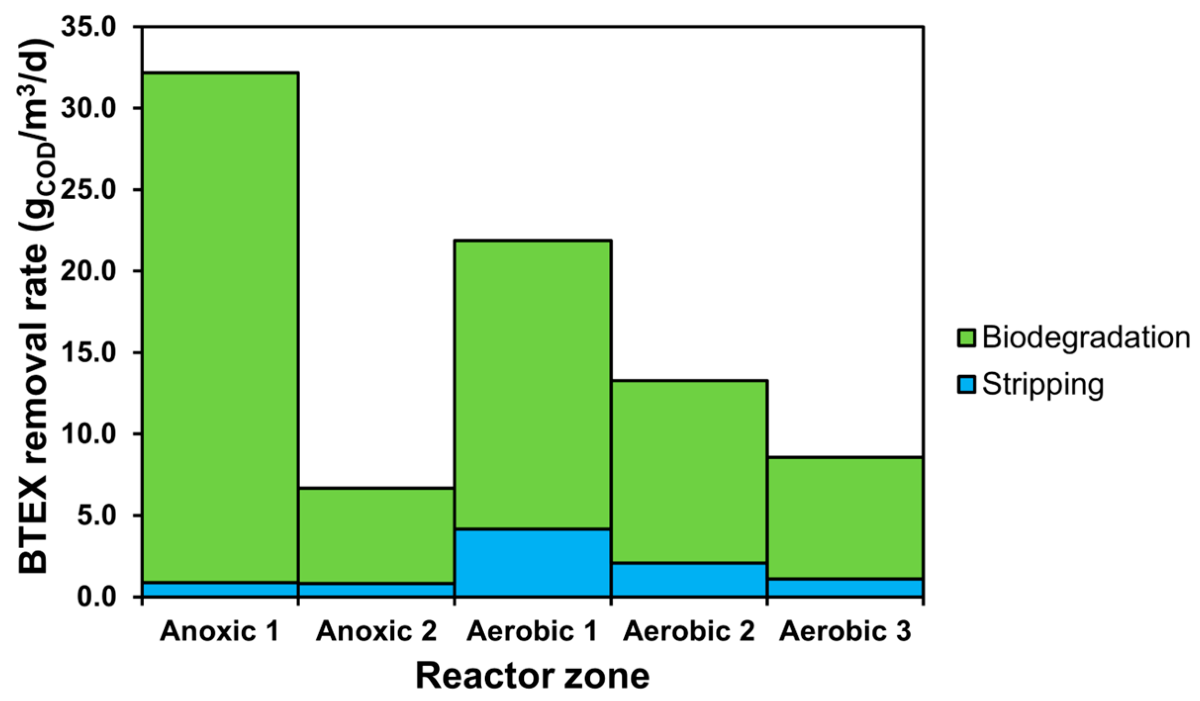
Figure 3.
Specific AC demand and blower energy demand for SRT-based scenarios.

Figure 4.
Effluent quality concerning BTEX compounds for SRT-based scenarios.
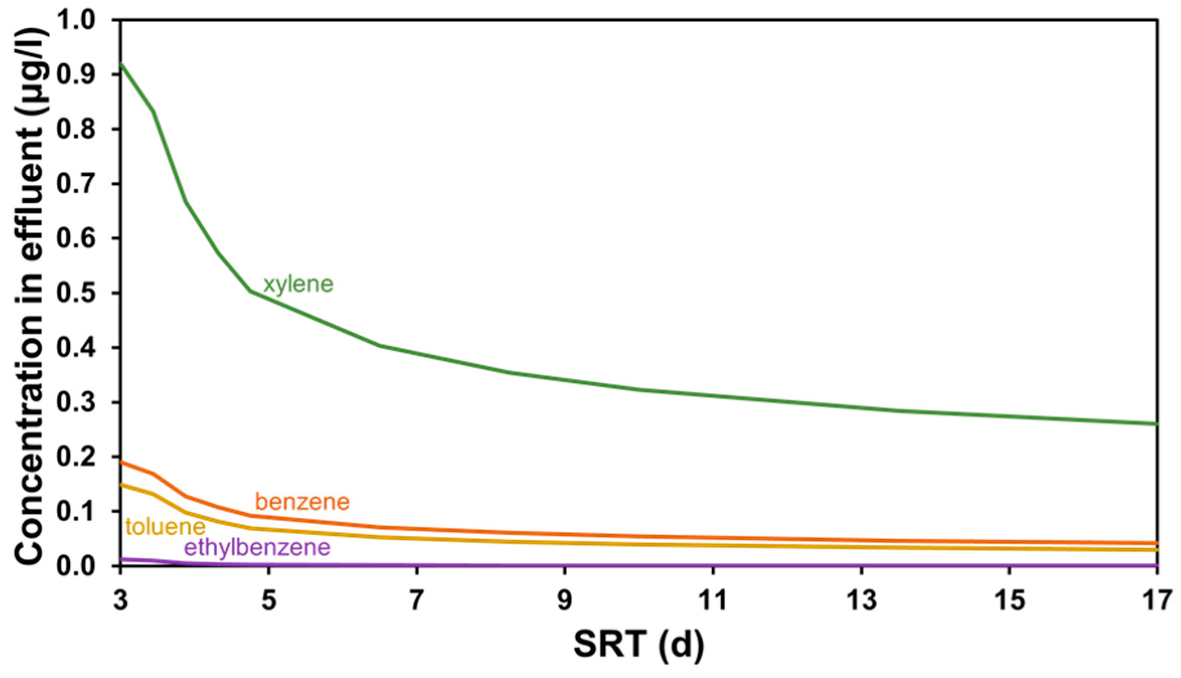
Figure 5.
Contribution of BTEX removal processes for SRT-based scenarios.
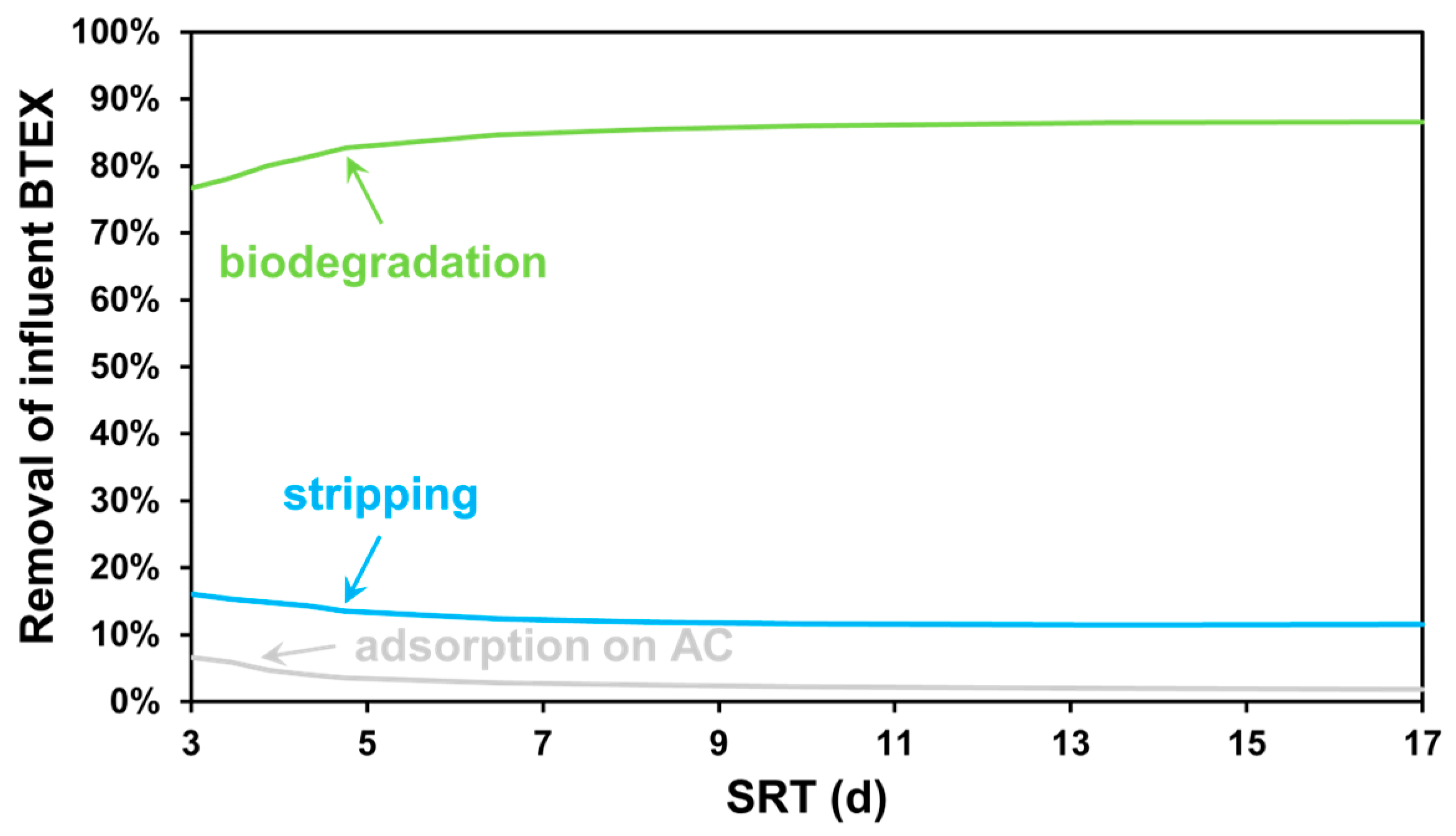
Figure 6.
Specific AC demand and blower energy demand for air flux-based scenarios.
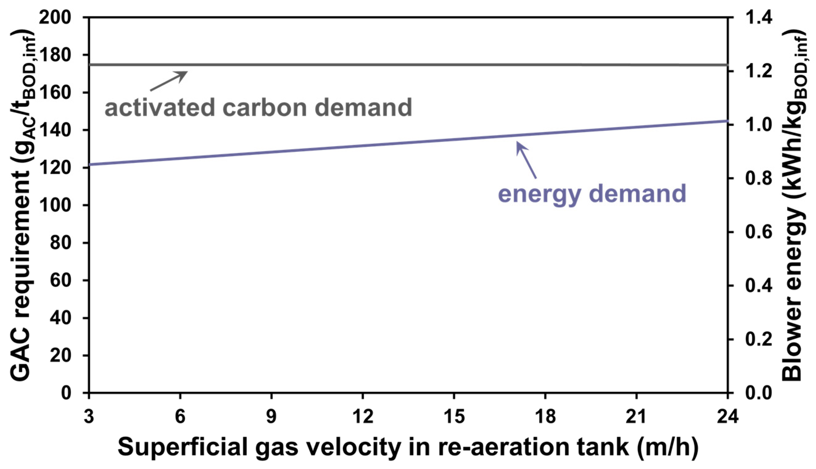
Figure 7.
Effluent quality concerning BTEX compounds for air flux-based scenarios.

Figure 8.
Contribution of BTEX removal processes for air flux-based scenarios.
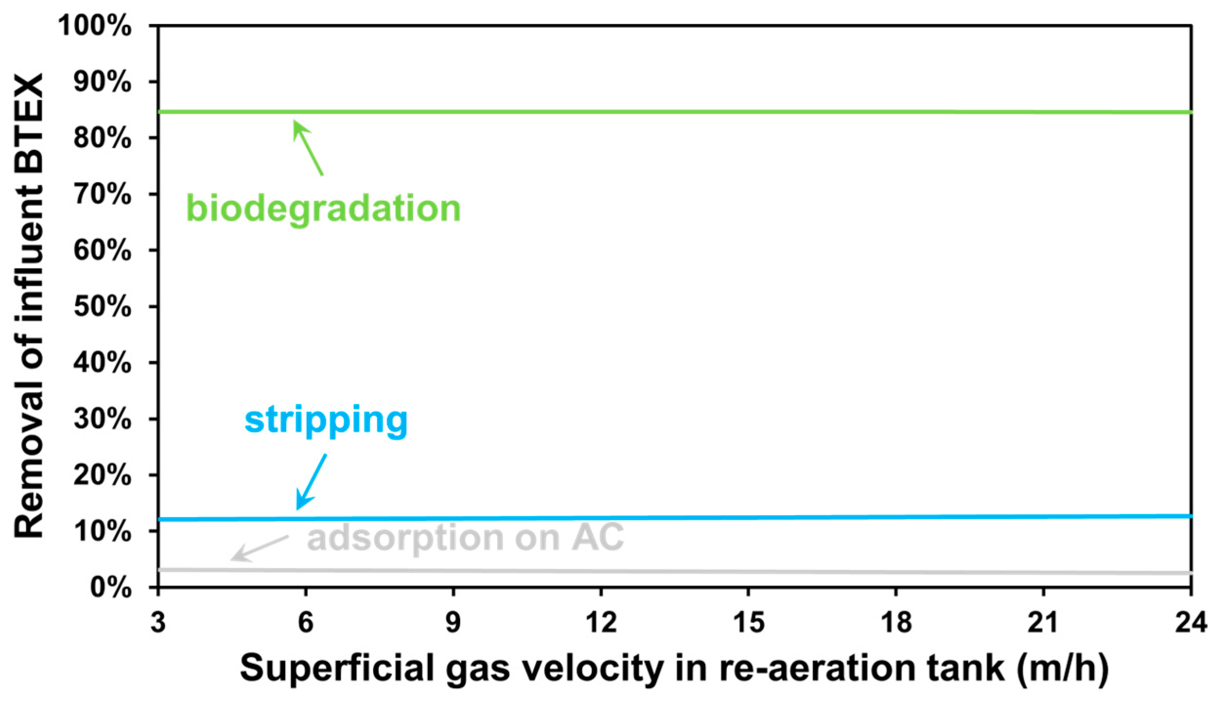
Figure 9.
Illustration of GAC tower operational strategies.
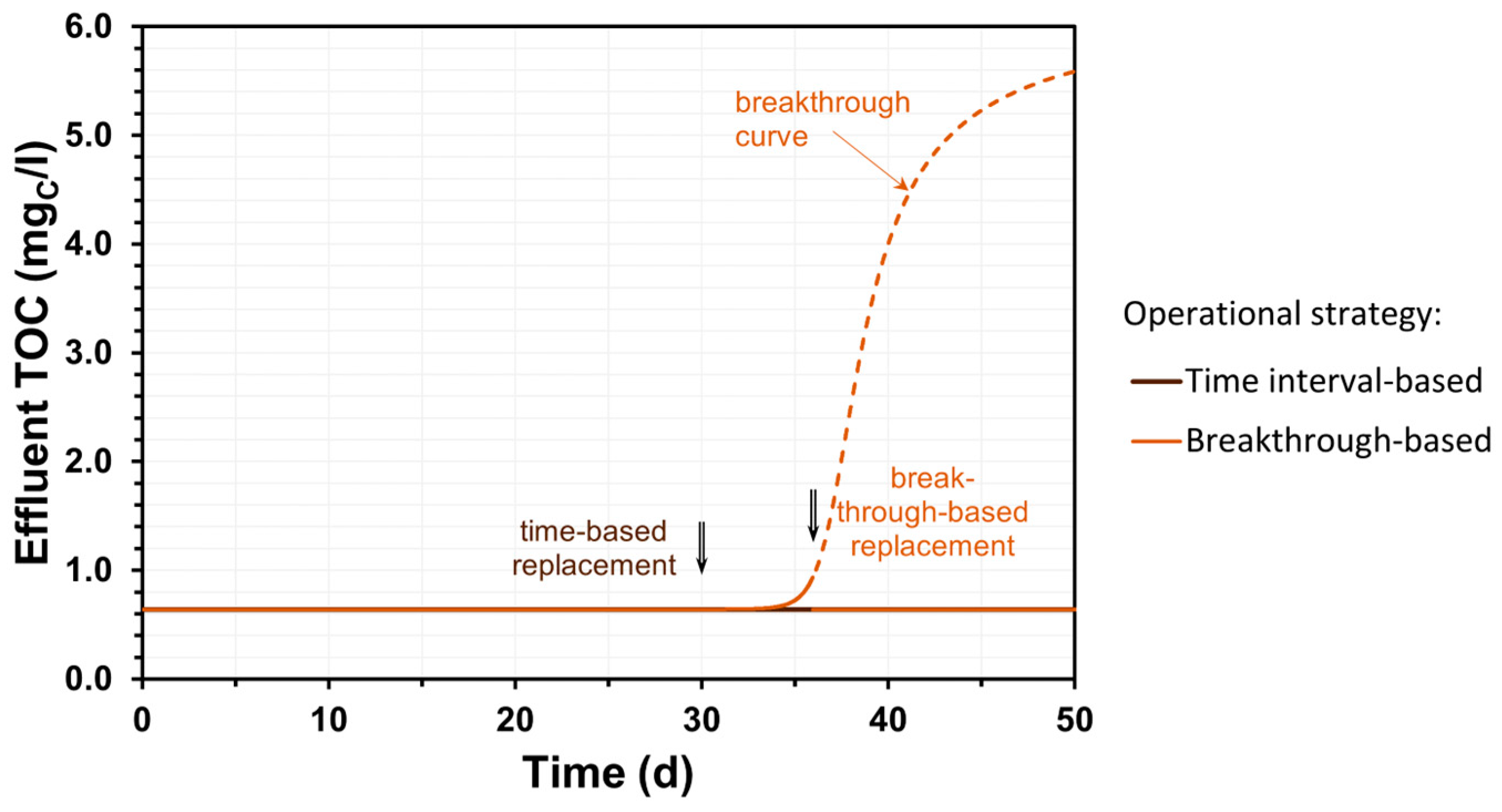
Table 1.
Main input parameters of the BSM1 test configuration.
| Parameter | Value | Unit |
|---|---|---|
| Influent properties | ||
| Flow | 18,446 | m3 d−1 |
| COD | 360 | gCOD m−3 |
| Filtered COD | 144 | gCOD m−3 |
| TOC | 114 | gC m−3 |
| TKN | 47 | gN m−3 |
| NH4-N | 30 | gN m−3 |
| Tank dimensions | ||
| Anoxic 1 zone volume | 1000 | m3 |
| Anoxic 2 zone volume | 1000 | m3 |
| Aerobic 1 zone volume | 1333 | m3 |
| Aerobic 2 zone volume | 1333 | m3 |
| Aerobic 3 zone volume | 1333 | m3 |
| Clarifier surface area | 1500 | m2 |
| Clarifier depth | 4 | m |
Disclaimer/Publisher’s Note: The statements, opinions and data contained in all publications are solely those of the individual author(s) and contributor(s) and not of MDPI and/or the editor(s). MDPI and/or the editor(s) disclaim responsibility for any injury to people or property resulting from any ideas, methods, instructions or products referred to in the content. |
© 2024 by the authors. Licensee MDPI, Basel, Switzerland. This article is an open access article distributed under the terms and conditions of the Creative Commons Attribution (CC BY) license (https://creativecommons.org/licenses/by/4.0/).
Share and Cite
MDPI and ACS Style
Bencsik, D.; Wadhawan, T.; Házi, F.; Karches, T. Plant-Wide Models for Optimizing the Operation and Maintenance of BTEX-Contaminated Wastewater Treatment and Reuse. Environments 2024, 11, 88. https://doi.org/10.3390/environments11050088
AMA Style
Bencsik D, Wadhawan T, Házi F, Karches T. Plant-Wide Models for Optimizing the Operation and Maintenance of BTEX-Contaminated Wastewater Treatment and Reuse. Environments. 2024; 11(5):88. https://doi.org/10.3390/environments11050088
Chicago/Turabian StyleBencsik, Dániel, Tanush Wadhawan, Ferenc Házi, and Tamás Karches. 2024. "Plant-Wide Models for Optimizing the Operation and Maintenance of BTEX-Contaminated Wastewater Treatment and Reuse" Environments 11, no. 5: 88. https://doi.org/10.3390/environments11050088
Note that from the first issue of 2016, this journal uses article numbers instead of page numbers. See further details here.