Article

A Simple Approach of Groundwater Quality Analysis, Classification, and Mapping in Peshawar, Pakistan

1
School of Forest Sciences, University of Eastern Finland, P.O. Box 111, 80101 Joensuu, Finland
2
Institute of Geographical Information Systems, National University of Sciences and Technology, Islamabad 44000, Pakistan
3
Department of Environmental Sciences, University of Peshawar, Peshawar 25000, Pakistan
4
College of Environmental Sciences and Engineering, Guilin University of Technology, Guilin 541004, China
5
School of Natural Sciences, Bangor University, Bangor, Gwynedd LL57 2DG, UK
*
Author to whom correspondence should be addressed.
Environments 2019, 6(12), 123; https://doi.org/10.3390/environments6120123
Submission received: 5 November 2019 / Revised: 27 November 2019 / Accepted: 3 December 2019 / Published: 7 December 2019
(This article belongs to the Special Issue Groundwater Quality and Groundwater Vulnerability Assessment)

Abstract

:
Groundwater is an important source of water for drinking, agriculture, and other household purposes, but high population growth, industrialization, and lack of oversight on environmental policies and implementation have not only degraded the quality but also stressed the quantity of this precious source of water. Many options existed, but this study evaluated, classified, and mapped the quality of groundwater used for potable consumption with a simple approach in an urban area (Peshawar valley) of Pakistan. More than 100 groundwater samples were collected and analyzed for physio-chemical parameters in a laboratory. Hierarchal clustering analysis (HCA) and classification and regression tree (CART) analysis were sequentially applied to produce potential clusters/groups (groundwater quality classes), extract the threshold values of the clusters, classify and map the groundwater quality data into meaningful classes, and identify the most critical parameters in the classification. The HCA produced six distinct potential clusters. We found a high correlation of electrical conductivity with t o t a l   h a r d n e s s ( R 2 =   0.72 ), a l k a l i n i t y ( R 2 =   0.59 ) and c h l o r i d e   ( R 2 =   0.64 ) , and, t o t a l   h a r d n e s s with c h l o r i d e ( R 2 = 0.62), and a l k a l i n i t y ( R 2 = 0.51). The CART analysis conclusively identified the threshold values of the six classes and showed that t o t a l   h a r d n e s s was the most critical parameter in the classification. The majority of the groundwater was either with worse quality or good quality, and only a few areas had the worst groundwater quality. This study presents a simple tool for the classification of groundwater quality based on several aesthetic constituents and can assist decision makers develop and support policies and/or regulations to manage groundwater resources.

1. Introduction

Groundwater plays a vital role in the water cycle, preserves a healthy ecosystem balance [1], and acts as one of the primary sources of drinking water [2], irrigation [3], and inflow to many streams or rivers [4,5]. However, uncontrolled and unregulated exploitation of groundwater [6], high population growth [7,8,9], rapid urbanization [10], expanding agriculture [11], and increased industrial development [12] is deteriorating this resource. Approximately 35% of the global population faces water stress [2], particularly in the central US, India, North-East China, and South Africa [13]. Pakistan also faces the same water-related challenges where the per capita water availability has decreased from 2172 to 1306 cubic meters per inhabitant in 25 years (1990–2015). Also, the majority of the population do not have access to safe drinking water (27.2 million) and sanitation (52.7 million), 0.039 million children under the age of five die every year from diarrhea [14], and three million people per year suffer from water-borne diseases [15]. It shows the poor management of drinking water quality where the standards of various parameters set by the World Health Organization [16] are recurrently neglected.
The drinking water is contaminated with chloride, toxic metals, nitrate, pesticides, and coliforms by various sources like unsafe handling and storage of households and industrial effluents, and agrochemical applications in agricultural fields [14]. The water quality parameters can have various positive or negative effects. For example, n i t r a t e concentration higher than 50 mg/L as nitrate causes methemoglobinemia (blue-baby syndrome) and thyroid effects in bottle-fed infants (less than six months old) [16,17], and it is advisable that concentrations should be less than 20 mg/L as nitrate [18]. H a r d n e s s (presence of magnesium) in the drinking water has a significant protective effect from cardiovascular diseases [19,20], while calcium hardness may cause scale deposition in pipes and tanks [16]. Nitrate in groundwater may originate from natural as well as anthropogenic sources, for example, geologic deposits in the form of sodium nitrate, standing water in the rice fields where blue-green algae assimilate atmospheric nitrate for tissue growth and after the degradation, released it to the soil and ultimately reach to the groundwater, nitrogen fertilizers in the agricultural fields, inappropriate human wastes disposal (septic tanks), and food processing industries [21]. Despite the harmful effects on human health, c h l o r i d e , which originates from landfill leachates, inorganic fertilizers in agricultural fields, infiltration of road de-icing salts, septic tank and industrial effluents, animal feeds, and irrigation drainage [22], produces a salty taste in water when it exceeds 250 mg/L [23] and can cause damage to the aquatic system [24] and terrestrial plant composition[25]. Analyzing the physio-chemical properties of drinking water could help in ascertaining the extent of pollution [26].
Groundwater vulnerability to pollution can be assessed by three significant approaches [27], for example, (a) overlay and index method, (b) process-based simulation methods, and (c) statistical methods. The overly and indexed methods combine various hydro-geologic attributes, such as geology, soil, phreatic level, groundwater recharge, and aquifer material. Each attribute is divided into different ranges or material types, and a subjective rating is assigned to each range or material type. Then, a weight is given to each attribute to enhance its importance according to the hydrogeologic setting of the area. Examples of this method include California Hotspot [28], DRASTIC (In the DRASTIC, each letter represents a parameter: Depth to groundwater/Phreatic level, net Recharge, Aquifer media, Soil media, Topography, Impact of vados zone and hydraulic Conductivity) model [29] or GIS-based DRASTIC models [30,31,32,33], Underground Injection Control (UIC) [34], and Iowa Ground Water Vulnerability [35]. The process-based simulation methods, such as MOUSE (Model of Underground Solute Evaluation)[36] and RUSTIC (Risk of Unsaturated/Saturated Transport and Transformation of Chemical Concentrations) [37], predict the contaminant transport processes using mathematical models. These methods replicate the actual physical and chemical properties of the pollutant transport and predict the degradation as it travels through the subsurface. These computations are not based on expert knowledge but on scientific principles, which control the movement of water and pollutant in the subsurface. The statistical methods, for example, regression analysis [38], discriminant analysis [39], classification and regression tree (CART) [40], and hierarchal clustering analysis (HCA) [26] utilize data from known locations and provide the categorization based on similarities or dissimilarities for the same geographic location from which the data were collected. As the statistical methods are based on the actual measurement of the water quality parameters, the validity and credibility of this approach are better than the overlay and indexed methods.
This study focuses on the statistical method and utilizes the clustering analysis with a simple approach that can easily be applied to any other area. The aim of the study is to determine the most commonly used physio-chemical properties of groundwater quality, including p H , electrical conductivity ( E C ; μS/cm), total dissolved solids ( T D S ; mg/L), bicarbonate a l k a l i n i t y ( H C O 3 ; mg/L as CaCO3), t o t a l   h a r d n e s s (mg/L as CaCO3), calcium hardness ( C a ; mg/L as CaCO3), magnesium hardness ( M g ; mg/L as CaCO3), t u r b i d i t y (Nephelometric Turbidity Unit/NTU), n i t r a t e (mg/L), and c h l o r i d e (mg/L) [41] in the Peshawar, which is the capital and most populated district of the province, utilize them in the clustering analysis, and classify the quality of groundwater into different and useful classes. We hypothesize that a useful tool for identifying groundwater quality groups can be developed from HCA and CART using easily obtained groundwater parameters. This would help the water-related agencies to act timely and efficiently in the worst groundwater quality areas as well as could be useful for planning a more detailed field classification when developing new groundwater supplies.

2. Material and Methods

2.1. Study Area

Peshawar (34°00′56.2″ N, 71°34′39.8″ E) is the most populated district and capital of the Khyber Pakhtunkhwa province in Pakistan. It spreads over an area of 1257 km2 [42] and has been divided into four towns (Town 1, Town 2, Town 3, Town 4) and a cantonment area which occupy 3%, 16%, 35%, 45%, and 1% of the total area, respectively [43]. These four towns are further subdivided into 83 union councils (Figure 1). The total population of the area is 4.269 million, wherein 2.299 million are living in rural areas and 1.970 million in urban areas [44]. The study area’s mean annual minimum and maximum temperatures are 1.0 °C and 42.3 °C [45], and the mean annual rainfall is 545.9 mm [46]. District Peshawar is the part of the large Peshawar basin, which has broad and oval-shaped depressions of fluvial, deltaic, and lacustrine sediments. The sediments are mainly gravel, sand, silt, and clay and form a moderate thick and productive aquifer in the north and center, approximately 50 to 100 m3/h yield while in the southern parts, the thickness of the aquifer is less and the yield is approximately 10–50 m3/h (Figure 2). These aquifers are mainly recharged by precipitation, surface water reservoirs, rivers, and irrigation network [47,48]. The underground rocks in the adjacent regions (eastern and southern) are limestones, shale, or calcareous quartzite [49]. Depth to groundwater table varies from 5 to more than 50 m from north-east to south-west [33].

2.2. Groundwater Sampling and Determination of Physio-Chemical Properties

A field survey was conducted in June 2012 to collect 105 groundwater samples from public drinking places, such as tube wells, dug wells, and hand pumps. These samples were collected in 250 mL plastic bottles from areas where depth to groundwater table was less than 5 m in the north while more than 50 m in the south-west. Before sampling, the bottles were thoroughly washed with distilled water to avoid the contamination. At least one ground sample was collected from each union council. However, few union councils, such as Adezai, Aza khel, Mashogagar, Mian Gujjar, Khatiki, and Joganaie, were inaccessible. Location (latitude and longitude) of each groundwater sample was recorded using a handheld global positioning system (GPS).
HACH Multimeter (Model SENSION 156) was used to measure p H , E C , and T D S of all 105 groundwater samples. However, before measurement, the Multimeter was calibrated with three buffer solutions (a solution with constant H ) such as 4, 7, and 10 to ensure the accurate readings. T u r b i d i t y was measured using HACH Turbidity meter (2100 N), C a and M g hardness, t o t a l   h a r d n e s s and c h l o r i d e with a titration method, while the nitrate concentration was determined through spectrophotometer (Thermo Spectronic, Genesys 5) [41].

2.3. The Clustering Analysis

Two types of clustering analysis, namely, hierarchal clustering analysis (HCA) and classification and regression tree (CART), were sequentially applied on the groundwater quality data to produce the potential clusters (groundwater quality classes) as well as to identify the most critical water quality parameters and their exact threshold values for the classification and mapping of groundwater quality. HCA is an unsupervised classification method which merges (agglomerative method) or splits (divisive method) the individual observations in a large group based on similar or dissimilar proximity measure, i.e., Euclidian distance (Equation (1)) [50].
d k l = m = 1 n ( X k m X l m ) 2
where, d k l is the Euclidian distance between observation k   and   l , X k m and X l m are the values of the mth variable.
In both cases, the HCA produces n number of clusters. Therefore, it is important to predetermine the optimal number of clusters ( O C ) [51]. The with-in cluster variation (sum of square) for 1–15 clusters was calculated to decide the O C as it provides excellent results with HCA [52].
The data was normalized (range-equalization) prior to Euclidian distance calculation because the parameters were in different units and treating them, in the same way, would produce uncertain results because one parameter would have more influence over other parameters [53]; thus, each value X was normalized to a scale of 0 to 1 (Equation (2)), according to their minimum and maximum values ( X m i n , X m a x ) (Table 1).
Z = ( X X m i n ) / ( X m a x X m i n )
After the normalization, function hclust included in package fastcluster [54] was applied, and the potential clusters ( O C ) were produced.
Since we were interested in identifying the most important water quality parameter and their exact threshold values for classification and mapping, CART analysis was used, and function rpart of the package Recursive Partitioning and Regression Trees (rpart; [40]) was applied. CART is a supervised classification method where the water quality parameters were used as explanatory variables, and the response variable was the potential clusters produced from HCA. CART uses all explanatory variables ( p H , E C , T D S , a l k a l i n i t y , t o t a l   h a r d n e s s , C a , M g , t u r b i d i t y , n i t r a t e , and c h l o r i d e ), calculates and ranks the impurity (heterogeneity) before and after each possible split (midpoint) for each explanatory variable, uses the value of that explanatory variable, which greatly reduces the heterogeneity, and divides the data into two homogeneous groups [55]. This recursive process is then applied on either side, and, at the end, a large tree is produced, which contains the exact threshold values of the explanatory variables at each split (node).

2.4. Classification and Mapping of the Groundwater Pollution

The threshold values of the water quality parameters (explanatory variables) at each node of the classification tree produced from CART analysis were used to extract and separate the whole data into those optimum clusters ( O C ; groundwater quality classes). The data were then imported to ArcGIS (version 10.4), and the union councils and water quality data were joined based on spatial location. Joining data based on spatial location has the advantage that inaccessible union councils with no groundwater sample get the ranking of the nearest sampling point, but the categorization of such inaccessible union councils can be considered as broad. This way, we used the identified classes and developed a thematic map of the groundwater quality; however, we assigned a high rank to those union councils that contained two or more groundwater samples with different groundwater quality classes.

3. Results and Discussion

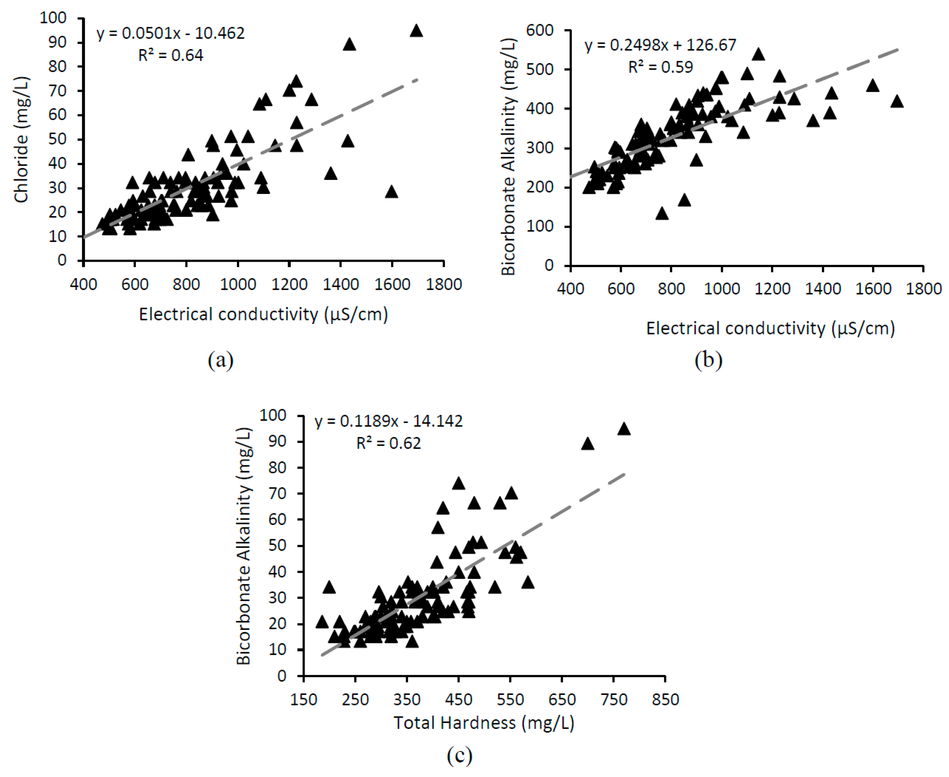
3.1. Physio-Chemical Properties of the Groundwater Samples

Table 1 shows a summary of the physio-chemical properties of the groundwater samples in the study area. The minimum, mean, and maximum values of the p H (7.1, 7.73, 8.08), n i t r a t e (3.60, 20.01, 41.73 mg/L), and c h l o r i d e (13.30, 30.13, 95.01 mg/L), and, mean value of t o t a l   h a r d n e s s (372.38 mg/L as CaCO3), t u r b i d i t y (0.89 NTU), T D S (393.01 mg/L), C a hardness (189.52 mg/L as CaCO3, and M g hardness (182.86 mg/L as CaCO3) were within permissible limits of drinking water quality standards. However, the later five parameters ( t o t a l   h a r d n e s s ,   t u r b i d i t y ,   T D S ,   C a ,   a n d   M g   h a r d n e s s ) contained groundwater samples with values higher than the drinking water quality standards. The mean values of the E C (809.44 μS/cm), which were much higher than the standard values (300–500 μS/cm), indicate salt enrichment in the study area [56]. The high level of such contaminants could be attributed to the domestic wastewater contamination from chemicals and woolen mills, soap, and marble industries [57] or the underground geology of the adjacent regions in which limestone/calcareous quartzite are the most common [49,58]. The results show that groundwater is safe for drinking in terms of nitrate concentration, which is the most important parameter in water quality assessment because its high concentration in drinking water affects bottle-fed infants, for example, cyanosis (discoloration of the skin) and methemoglobinemia [18].

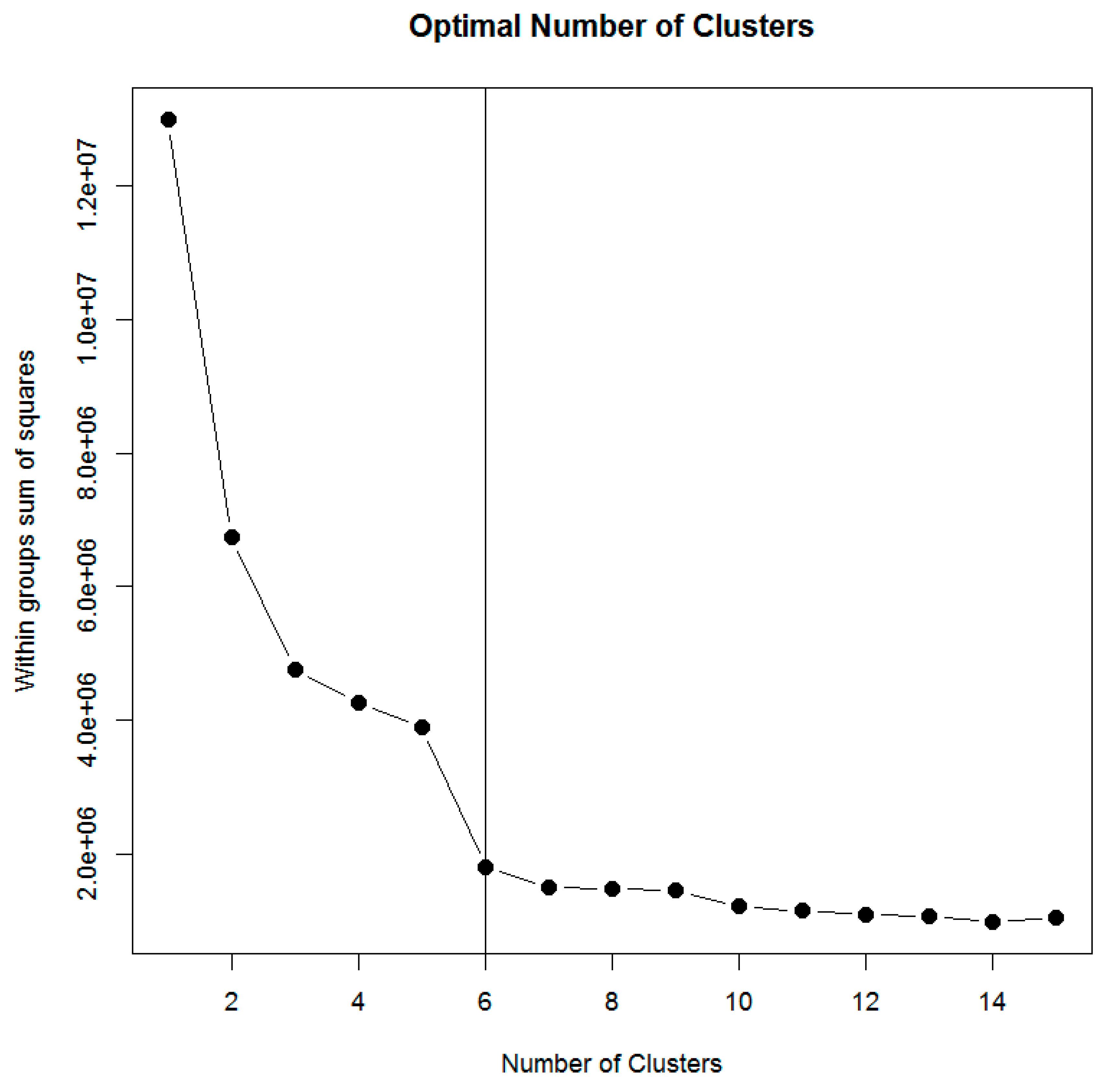
3.2. Clustering Analysis of the Groundwater Data

Many researchers have used the DRASTIC [29] or GIS-based DRASTIC models (overlay and indexed method) [30,31,32,33], MOUSE and RUSTIC models (process based simulation methods) [36,37] for water quality assessment while other have applied the clustering analysis (statistical methods) [32,60,61,62] in which they simply separated different clusters/groups based on similarity or dissimilarity. The clustering analysis is also used in this study, but the interest was to find out the exact threshold values that separate those clusters, and this makes it different than the other studies. Two types of clustering analysis such as HCA: an unsupervised statistical method which uses similarity, dissimilarity, or distance metrics and classify a large group of observations into several clusters [63,64,65] and CART: a statistical technique, which is used to select the most important parameters and their interactions in the determination of an outcome [40] were sequentially applied with a simple approach. First, HCA was used to separate the potential clusters (groundwater quality classes), and then, the CART analysis was used to extract the exact threshold values of those potential clusters for the classification and mapping of groundwater quality and identification of the most important parameters in the disintegration of clusters [51]. In HCA, it was challenging to decide the optimum number of clusters; however, the within-cluster variation (sum of square), which produces satisfactory results with hierarchal clustering [52], was used and calculated from 1 to 15 clusters (Figure 3). A high variation (within groups sum of square) in the water quality existed from cluster 1 to 6, but from cluster 6 onwards, the variation was small. Thus, we decided to use an optimum number of clusters O C = 6 .
Then, the HCA [54] was applied on water quality data, which included all the water quality parameters - p H , E C , T D S , H C O 3 , t o t a l   h a r d n e s s , C a , M g , t u r b i d i t y , n i t r a t e , and c h l o r i d e - and six potential clusters/groups were produced, wherein, some groups were clearly distinguishable on the scatterplot while others had some degree of overlaps (Figure 4). Only the most correlated parameters ( E C , a l k a l i n i t y , and c h l o r i d e s ) are presented on the scatterplot as it was expected that these parameters would play an important role in the disintegration of the potential clusters/groups (see below). A high correlation of E C with c h l o r i d e (R2 = 0.64) and a l k a l i n i t y (R2 = 0.59), and t o t a l   h a r d n e s s with a l k a l i n i t y (R2 = 0.62) (Figure 5) was found. Thus, E C and t o t a l   h a r d n e s s could be the key parameters in the water quality assessment [17]. A similar high relationship was also found by [66] during the physio-chemical analysis of groundwater in Chithar Riber Basin, India. The high correlation of the E C with c h l o r i d e and a l k a l i n i t y also shows that the salinity in the study area’s groundwater is controlled by chlorides and bicarbonates [60]. This could probably be derived from weathering of rock salts and gypsum-bearing aquifers [67]. Also, the sewage water, which contains untreated effluents from small industries, such as marble, soap, and food processing, is used for agriculture purposes in the study area, and it contaminates the crops as well as the groundwater [68]. Pakistan council of research in water resources [69] has described that the groundwater of Peshawar is dominated by M g and C a cations as well as chloride and bicarbonate anions; however, our results showed the most of them are within the permissible limits.
After the HCA, the exact threshold values of the groundwater quality parameters, which separated the clusters, were extracted, and the classification tree, which was produced as a result of the CART analysis, is shown in Figure 6. As expected, the first split/node was based on t o t a l   h a r d n e s s 265   mg / L as CaCO3, which separated the whole data into two groups. The next splits were based on E C < 1432   μ S / cm , c h l o r i d e 35   mg / L , and E C 939   μ S / cm . Moreover, on the other side of the classification tree, the split was based on n i t r a t e 18   mg / L . CART analysis produced six potential groups/clusters, identified the threshold values of water quality parameters and showed that t o t a l   h a r d n e s s was the most important parameter in the disintegration of the potential clusters/groups as the first split was based on the t o t a l   h a r d n e s s [40]. CART analysis performed smart decisions and included the high correlated parameters, which were expected to be important in the classification of groundwater quality into useful classes.

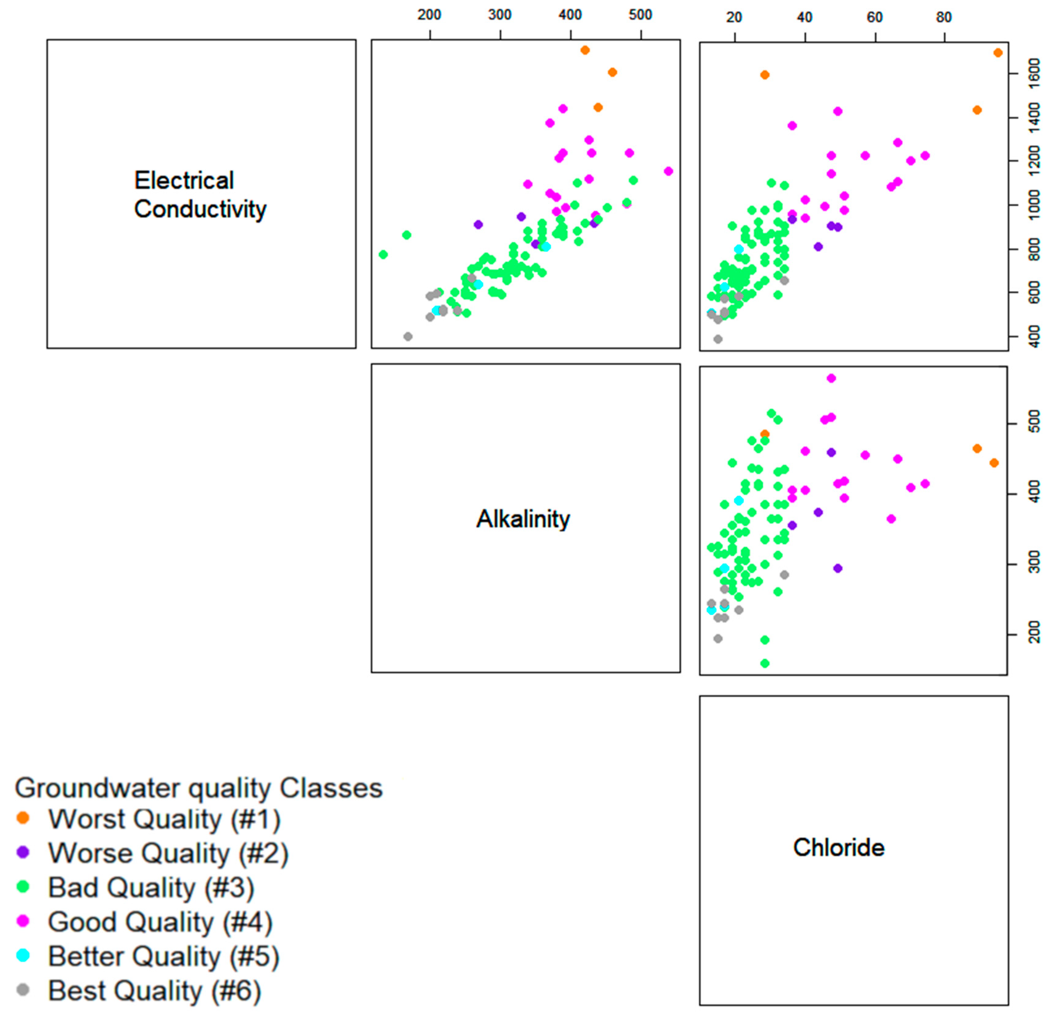
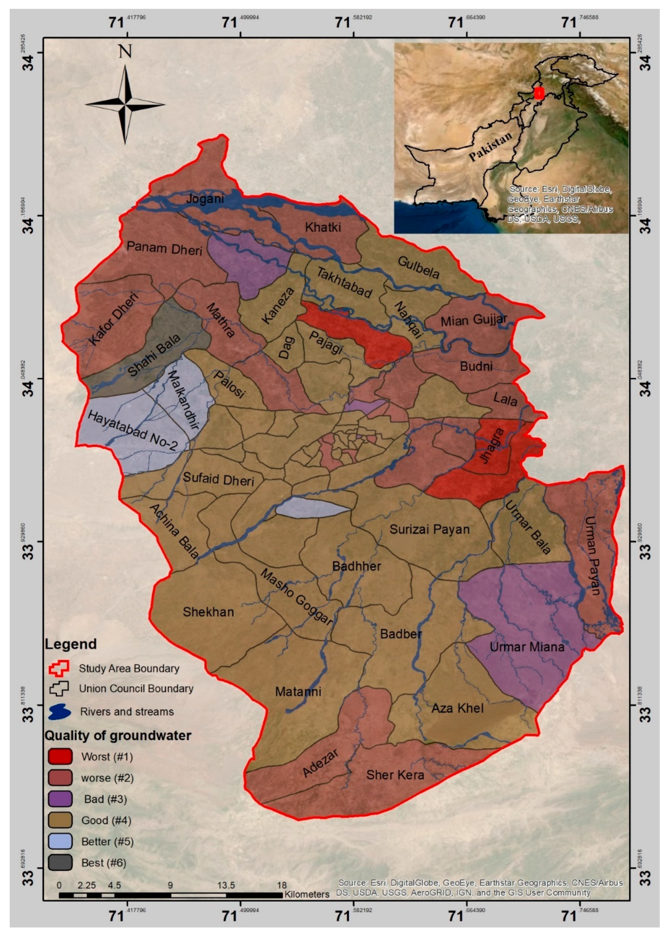
3.3. Classification and Mapping of the Groundwater Pollution

The threshold values of the water quality parameter at each node/split of the classification tree as identified by CART analysis (Figure 6) were used to divided the whole data into six classes and were named according to the level of concentration of the water quality parameters, such as worst quality (#1), worse quality (#2), bad quality (#3), good quality (#4), better quality (#5), and best quality (#6). Figure 7 shows the mean values of the groundwater quality parameters of each groundwater quality class and their standard deviations, wherein, the values of the parameters, particularly, the E C ,   a l k a l i n i t y , and c h l o r i d e , are clearly decreasing from the worst quality class (#1) to the best quality class (#6) (Figure 7a). The thematic map of the final classes of the groundwater quality in the study area (Figure 8) shows that the worst (#1) and worse (#2) groundwater quality areas (19 union councils) are located in the north, center, south, and south-eastern parts of the study area, and the bad quality (#3) areas are Urmar Miana and Chaghar Matti located at the north and south, respectively. The low groundwater quality at the north and north-eastern parts (worst (#1) and worse (#2) quality areas) are probably due to the fertilizers and pesticides applications in the agricultural fields or domestic and industrial wastewater, which drains into the river in these areas [59] coupled with the lowest groundwater table (less than 1.5 m), sandy soil type, and gravel and sand aquifer material where the contaminants require the shortest travel time to reach the groundwater and move easily from one place to another [33]. Most of the area is under good groundwater quality (#4) (eastern, central, south-eastern areas and some parts of the south and north-east) where the water table is more than 50 m deep [70] and the soil type is silt-loam which helps to restrict or minimize the movement of the contaminants [33]. Three union councils such as Hayatabad, Malakandir, and Bazid Khel have better groundwater quality (#5), and only the Shahi Bala union council has the best groundwater quality (#6). This categorization can be considered as broad in the union councils such as Sher Kera, Aza Khel, and Shekhan (south-west), and Khatki, Mian Gujjar, Lala, and Jhagra (north-east) where the data was not available, and a detailed water quality analysis will be recommended before planning a water supply scheme. The thematic map produced as a result of the clustering analysis has a similar spatial distribution of the groundwater quality as the final vulnerability map in [33], in which they have assessed the groundwater vulnerability to pollution using a completely different method (GIS-based DRASTIC model). It is also interesting to compare the thematic map of groundwater quality classes (Figure 8) with the spatial distribution maps of different water quality parameters in the study area [12]. This method was able to identify and separate all areas with a high concentration of the water quality parameters as worse or worst groundwater quality class. The groundwater quality spatial distribution could further be improved if additional water quality parameters are included in the analysis; however, the field survey and laboratory analysis are the most tedious job and depend on the time and cost involved [71]. It would also be more interesting to perform a spatiotemporal analysis of the groundwater quality in the study area to observe a periodical change in the groundwater quality and validate the performance of the method used. We believe that the clustering analysis used in this study would be a simple and robust way for water-related agencies to classify, map, and prioritize groundwater quality.

4. Conclusions

In this study, a useful tool that could be applied to any area was developed from HCA and CART analysis to identify different groundwater quality classes. Simple and easily obtained groundwater quality parameters, such as p H , E C ,   T D S ,   a l k a l i n i t y , t o t a l   h a r d n e s s , C a , M g , t u r b i d i t y , n i t r a t e , and c h l o r i d e were determined and used as input in the tool. This tool could be used as a groundwater quality identifier before developing new water supplies; however, adding additional groundwater quality parameters will further improve the results. The tool can also be used for prioritizing the groundwater quality regions, and its validity can be assessed by planning a detailed spatiotemporal analysis of the groundwater quality in the same or any other region.

Author Contributions

Conceptualization: S.A. and R.V.; data curation: M.S.B. and A.S.; formal analysis: S.A., M.S.B. and A.S.; methodology: M.S.B. and A.S.; supervision: J.I., M.M. and R.V.; writing—original draft: S.A.; writing—review and editing: J.I., M.M. and R.V.

Funding

This research received no external funding

Acknowledgments

The authors would like to thank the Institute of Environmental Sciences and Engineering (IESE), National University of Sciences and Technology, Islamabad, Pakistan for providing the facility of laboratory analysis.

Conflicts of Interest

The authors declare no conflict of interest.

References

  1. Cui, Y.; Shao, J. The role of ground water in arid/semiarid ecosystems, Northwest China. Groundwater 2005, 43, 471–477. [Google Scholar] [CrossRef]
  2. Ahmed, M.F.; Ahuja, S.; Alauddin, M.; Hug, S.J.; Lloyd, J.R.; Pfaff, A.; Pichler, T.; Saltikov, C.; Stute, M.; van Geen, A. Ensuring safe drinking water in Bangladesh. Science 2006, 314, 1687–1688. [Google Scholar] [CrossRef] [PubMed] [Green Version]
  3. Siebert, S.; Burke, J.; Faures, J.M.; Frenken, K.; Hoogeveen, J.; Döll, P.; Portmann, F.T. Groundwater use for irrigation—A global inventory. Hydrol. Earth Syst. Sci. 2010, 14, 1863–1880. [Google Scholar] [CrossRef] [Green Version]
  4. Cook, P.G.; Favreau, G.; Dighton, J.C.; Tickell, S. Determining natural groundwater influx to a tropical river using radon, chlorofluorocarbons and ionic environmental tracers. J. Hydrol. 2003, 277, 74–88. [Google Scholar] [CrossRef]
  5. Cook, P.G.; Wood, C.; White, T.; Simmons, C.T.; Fass, T.; Brunner, P. Groundwater inflow to a shallow, poorly-mixed wetland estimated from a mass balance of radon. J. Hydrol. 2008, 354, 213–226. [Google Scholar] [CrossRef]
  6. Qureshi, A.S. Challenges and Opportunities of Groundwater Management in Pakistan. In Groundwater of South Asia; Mukherjee, A., Ed.; Springer: Singapore, 2018; pp. 735–757. [Google Scholar] [CrossRef]
  7. Alcamo, J.; Henrichs, T.; Rösch, T. World Water in 2025: Global Modeling and Scenario Analysis for the World Commission on Water for the 21st Century; Kassel World Water Ser. Rep. 2; Center for Environmental Systems Research; University of Kassel: Kassel, Germany, 2000. [Google Scholar]
  8. Vörösmarty, C.J.; Green, P.; Salisbury, J.; Lammers, R.B. Global water resources: Vulnerability from climate change and population growth. Science 2000, 289, 284–288. [Google Scholar] [CrossRef] [Green Version]
  9. Zhang, Q.; Li, Z.; Zeng, G.; Li, J.; Fang, Y.; Yuan, Q.; Wang, Y.; Ye, F. Assessment ofsurface water quality using multivariate statistical techniques in red soil hilly region: A case study of Xiangjiang watershed, China. Environ. Monit. Assess. 2009, 152, 123. [Google Scholar] [CrossRef]
  10. Daud, M.K.; Nafees, M.; Ali, S.; Rizwan, M.; Bajwa, R.A.; Shakoor, M.B.; Arshad, M.U.; Chatha, S.A.S.; Deeba, F.; Murad, W.; et al. Drinking water quality status and contamination in Pakistan. BioMed Res. Int. 2017, 2017, 7908183. [Google Scholar] [CrossRef]
  11. Wada, Y.; van Beek, L.P.; van Kempen, C.M.; Reckman, J.W.; Vasak, S.; Bierkens, M.F. Global depletion of groundwater resources. Geophys. Res. Lett. 2010, 37. [Google Scholar] [CrossRef] [Green Version]
  12. Adnan, S.; Iqbal, J. Spatial analysis of the groundwater quality in the Peshawar District, Pakistan. Procedia Eng. 2014, 70, 14–22. [Google Scholar] [CrossRef] [Green Version]
  13. Hanasaki, N.; Kanae, S.; Oki, T.; Masuda, K.; Motoya, K.; Shirakawa, N.; Shen, Y.; Tanaka, K. An integrated model for the assessment of global water resources—Part 2: Applications and assessments. Hydrol. Earth Syst. Sci. 2008, 12, 1027–1037. [Google Scholar] [CrossRef] [Green Version]
  14. UNDP Pakistan. Development Advocate Pakistan: Water Security in Pakistan: Issues and Challenges; United Nations Development Programme Pakistan: Islamabad, Pakistan, 2017; Volume 3, Issue 4, Available online: https://www.pk.undp.org/content/pakistan/en/home/library/development_policy/development-advocate-pakistan--volume-3--issue-4.html (accessed on 5 October 2019).
  15. PRI—Million Sick Due to Lack of Water in Pakistan. Available online: http://www.pri.org/stories/2009-04-20/millions-sick-due-lack-clean-water-pakistan (accessed on 2 June 2019).
  16. World Health Organization. Guidelines for Drinking-Water Quality, 4th ed.; incorporating the first addendum; Licence: CC BY-NC-SA 3.0 IGO; World Health Organization: Geneva, Switzerland, 2017. [Google Scholar]
  17. Anku, Y.S.; Banoeng-Yakubo, B.; Asiedu, D.K.; Yidana, S.M. Water quality analysis of groundwater in crystalline basement rocks, Northern Ghana. Environ. Geol. 2009, 58, 989–997. [Google Scholar] [CrossRef]
  18. Comly, H.H. Cyanosis in infants caused by nitrates in well water. J. Am. Med. Assoc. 1945, 129, 112. [Google Scholar] [CrossRef]
  19. Biorck, G.; Bostrom, H.; Widstrom, A. On the relationship between water hardness and death rate in cardiovascular disease. Acta Med. Scand. 1965, 178, 239–252. [Google Scholar] [CrossRef] [PubMed]
  20. Yang, C.Y. Calcium and magnesium in drinking water and risk of death from cerebrovascular disease. Stroke 1998, 29, 411–414. [Google Scholar] [CrossRef] [PubMed] [Green Version]
  21. Bouchard, D.C.; Williams, M.K.; Surampalli, R.Y. Nitrate contamination of groundwater: Sources and potential health effects. J. -Am. Water Work. Assoc. 1992, 84, 85–90. [Google Scholar] [CrossRef]
  22. Yamakanamardi, S.V.; Hampannavar, U.S.; Purandara, B.K. Assessment of chloride concentration in groundwater: A case study for Belgaum City. Int. J. Environ. Sci. 2011, 2, 271. [Google Scholar]
  23. Cronin, A.A.; Hoadley, A.W.; Gibson, J.; Breslin, N.; Komou, F.K.; Haldin, L.; Pedley, S. Urbanisation effects on groundwater chemical quality: Findings focusing on the nitrate problem from 2 African cities reliant on on-site sanitation. J. Water Health 2007, 5, 441–454. [Google Scholar] [CrossRef] [Green Version]
  24. Kaushall, S.; Groffman, P.; Likens, G.; Belt, K.; Stack, W.; Kelly, V.; Band, L.; Fisher, G. Increased salinization of freshwater in the Northeastern United States. Proc. Natl. Acad. Sci. USA 2005, 102, 13517–13520. [Google Scholar] [CrossRef] [Green Version]
  25. Miklovic, S.; Galatowitsch, S. Effect of NaCl and Typha angustifolia L. on marsh community establishment: A greenhouse study. Wetlands 2005, 24, 420–429. [Google Scholar] [CrossRef] [Green Version]
  26. Omo-Irabor, O.O.; Olobaniyi, S.B.; Oduyemi, K.; Akunna, J. Surface and groundwater water quality assessment using multivariate analytical methods: A case study of the Western Niger Delta, Nigeria. Phys. Chem. Earthparts A/B/C 2008, 33, 666–673. [Google Scholar] [CrossRef]
  27. National Research Council. Groundwater Vulnerability Assessment: Contamination Potential under Conditions of Uncertainties; National Academy Press: Washington, DC, USA, 1993. [Google Scholar]
  28. Cohen, D.B.; Fisher, C.; Reid, M.L. Ground-water contamination by toxic substances: A California assessment. In Evaluation of Pesticides in Ground Water; Garner, W.Y., Honeycutt, R.C., Nigg, H.N., Eds.; ACS Symp. Series 315; American Chemical Society: Washington, DC, USA, 1986; pp. 499–529. [Google Scholar]
  29. Aller, L.; Lehr, J.H.; Petty, R.; Bennett, T. DRASTIC: A Standardized System to Evaluate Groundwater Pollution Potential Using Hydrogeologic Settings; National Water Well Association: Washington, OH, USA, 1987. [Google Scholar]
  30. Duarte, L.; Espinha Marques, J.; Teodoro, A.C. An Open Source GIS-Based Application for the Assessment of Groundwater Vulnerability to Pollution. Environments 2019, 6, 86. [Google Scholar] [CrossRef] [Green Version]
  31. Shirazi, S.; Imran, H.; Akib, S.; Yusop, Z.; Harun, Z. Groundwater vulnerability assessment in the Melaka State of Malaysia using DRASTIC and GIS techniques. Environ. Earth Sci. 2013, 70, 2293–2304. [Google Scholar] [CrossRef]
  32. Shahab, A.; Shihua, Q.; Rad, S.; Keita, S.; Khan, M.; Adnan, S. Groundwater vulnerability assessment using GIS-based DRASTIC method in the irrigated and coastal region of Sindh province, Pakistan. Hydrol. Res. 2019, 50, 319–338. [Google Scholar] [CrossRef] [Green Version]
  33. Adnan, S.; Iqbal, J.; Maltamo, M.; Valbuena, R. GIS-based DRASTIC model for groundwater vulnerability and pollution risk assessment in the Peshawar District, Pakistan. Arab. J. Geosci. 2018, 11, 458. [Google Scholar] [CrossRef] [Green Version]
  34. Pettyjohn, W.A.; Savoca, M.; Self, D. Regional Assessment of Aquifer Vulnerability and Sensitivity in the Conterminous United States; Report EPA-600/2-91/043; Environmental Protection Agency: Ada, OK, USA, 1991. [Google Scholar]
  35. Hoyer, B.E.; Hallberg, G.R. Ground Water Vulnerability Regions of Iowa; Special Map 11; Iowa Department of Natural Resources: Iowa, IA, USA, 1991. [Google Scholar]
  36. Steenhuis, T.S.; Pacenka, S.; Porter, K.S. MOUSE: A management model for evaluation ground water contamination from diffuse surface sources aided by computer graphics. Appl. Agric. Res. 1987, 2, 277–289. [Google Scholar]
  37. Dean, J.D.; Huyakorn, P.S.; Donigian, A.S., Jr.; Voos, K.A.; Schanz, R.W.; Meeks, Y.J.; Carsel, R.F. Risk of Unsaturated/Saturated Transport and Transformation of Chemical Concentrations (RUSTIC); EPA/600/3-89/048a; Environmental Protection Agency: Athens, GA, USA, 1989; Volumes I and II. [Google Scholar]
  38. Chen, H.; Druliner, A.D. Agricultural Chemical Contamination of Ground Water in Six Areas of the High Plains Aquifer, Nebraska. In National Water Summary 1986—Hydrologic Events and Ground-Water Quality; Water-Supply Paper 2325; Geological Survey: Reston, VA, USA, 1988. [Google Scholar]
  39. Teso, R.R.; Younglove, T.; Peterson, M.R.; Sheeks, D.L.; Gallavan, R.E. Soil taxonomy and surveys: Classification of areal sensitivity to pesticide contamination of ground water. J. Soil Water Conserv. 1988, 43, 348–352. [Google Scholar]
  40. Breiman, L.; Friedman, J.H.; Olshen, R.A.; Stone, C.J. Classification and Regression Trees; Wadsworth: Monterey, CA, USA, 1984. [Google Scholar]
  41. Eaton, A.D.; Cresceri, L.S.; Rice, E.W.; Greenberg, A.B. Standard Methods for the Examination of Water and Wastewater, 21st ed.; American Public Health Association: Washington, DC, USA, 2005. [Google Scholar]
  42. Ud Din, I.; Xue, M.C.; Abdullah, A.S.; Shah, T.; Ilyas, A. Role of information & communication technology (ICT) and e-governance in health sector of Pakistan: A case study of Peshawar. Cogent Soc. Sci. 2017, 3, 1308051. [Google Scholar]
  43. City Development Strategy Peshawar. 2001. Available online: http://documents.worldbank.org/curated/en/680651468287766516/pdf/563740v10REPLA00Box385328B00PUBLIC0.pdf (accessed on 16 August 2019).
  44. Pakistan Bureau of Statistics. Block Wise Provisional Summary Results of 6th Population & Housing Census-2017. 2018. Available online: http://www.pbs.gov.pk/content/block-wise-provisional-summary-results-6th-population-housing-census-2017-january-03-2018 (accessed on 26 May 2019).
  45. Mirza, M.W.; Abbas, Z.; Rizvi, M.A. Temperature zoning of Pakistan for asphalt mix design. Pak. J. Eng. Appl. Sci. 2016, 8, 49–60. [Google Scholar]
  46. Pakistan Meteorological Department. Rainfall Data of Peshawar Station (1977–2006) Collected from Pakistan Meteorological Department; Pakistan Meteorological Department: Islamabad, Pakistan, 2013. [Google Scholar]
  47. Hussain, A.; Dipietro, J.A.; Pogue, K.R. Stratigraphy and structure of the Peshawar Basin. Pakistan. J. Nepal. Geol. Soc. 1998, 18, 25–35. [Google Scholar]
  48. Yousafzai, A.; Eckstein, Y.; Dahl, P. Numerical simulation of groundwater flow in the Peshawar intermontane basin, northwest Himalayas. Hydrogeol. J. 2008, 16, 1395. [Google Scholar] [CrossRef]
  49. Pogue, K.R.; Wardlaw, B.R.; Harris, A.G.; Hussain, A. Paleozoic and Mesozoic stratigraphy of the Peshawar basin, Pakistan: Correlations and implications. Geol. Soc. Am. Bull. 1992, 104, 915–927. [Google Scholar] [CrossRef]
  50. Everitt, B.S.; Landau, S.; Leese, M.; Stahl, D. Hierarchical clustering. Cluster Analysis, 5th ed.; John Wiley & Sons, Ltd: Hoboken, NJ, USA, 2011; pp. 71–110. [Google Scholar]
  51. Tibshirani, R.; Walther, G.; Hastie, T. Estimating the number of clusters in a data set via the gap statistic. J. R. Stat. Soc. Ser. B 2001, 63, 411–423. [Google Scholar] [CrossRef]
  52. Sugar, C.A.; James, G.M. Finding the number of clusters in a dataset: An information-theoretic approach. J. Am. Stat. Assoc. 2003, 98, 750–763. [Google Scholar] [CrossRef]
  53. Milligan, G.W.; Cooper, M.C. A study of standardization of variables in cluster analysis. J. Classif. 1988, 5, 181–204. [Google Scholar] [CrossRef]
  54. Müllner, D. fastcluster: Fast hierarchical, agglomerative clustering routines for R and Python. J. Stat. Softw. 2013, 53, 1–18. [Google Scholar] [CrossRef] [Green Version]
  55. Lawrence, R.L.; Wright, A. Rule-based classification systems using classification and regression tree (CART) analysis. Photogramm. Eng. Remote Sens. 2001, 67, 1137–1142. [Google Scholar]
  56. Prasanth, S.S.; Magesh, N.S.; Jitheshlal, K.V.; Chandrasekar, N.; Gangadhar, K. Evaluation of groundwater quality and its suitability for drinking and agricultural use in the coastal stretch of Alappuzha District, Kerala, India. Appl. Water Sci. 2012, 2, 165–175. [Google Scholar] [CrossRef] [Green Version]
  57. Khan, S.; Rauf, R.; Muhammad, S.; Qasim, M.; Din, I. Arsenic and heavy metals health risk assessment through drinking water consumption in the Peshawar District, Pakistan. Hum. Ecol. Risk Assess. Int. J. 2016, 22, 581–596. [Google Scholar] [CrossRef]
  58. Ullah, Z.; Khan, H.; Waseem, A.; Mahmood, Q.; Farooq, U. Water quality assessment of the River Kabul at Peshawar, Pakistan: Industrial and urban wastewater impacts. J. Water Chem. Technol. 2013, 35, 170–176. [Google Scholar] [CrossRef] [Green Version]
  59. Pakistan Environmental Protection Agency. National Standards for Drinking Water Quality (NSDWG). 2008. Available online: http://www.freshwateraction.net/sites/freshwateraction.net/files/Drinking%20water%20in%20Pakistan.pdf (accessed on 21 September 2019).
  60. Bodrud-Doza, M.; Islam, A.T.; Ahmed, F.; Das, S.; Saha, N.; Rahman, M.S. Characterization of groundwater quality using water evaluation indices, multivariate statistics and geostatistics in central Bangladesh. Water Sci. 2016, 30, 19–40. [Google Scholar] [CrossRef] [Green Version]
  61. Nguyen, T.T.; Kawamura, A.; Tong, T.N.; Nakagawa, N.; Amaguchi, H.; Gilbuena, R., Jr. Clustering spatio—Seasonal hydrogeochemical data using self-organizing maps for groundwater quality assessment in the Red River Delta, Vietnam. J. Hydrol. 2015, 522, 661–673. [Google Scholar] [CrossRef]
  62. Hussain, M.; Ahmed, S.M.; Abderrahman, W. Cluster analysis and quality assessment of logged water at an irrigation project, eastern Saudi Arabia. J. Environ. Manag. 2008, 86, 297–307. [Google Scholar] [CrossRef] [PubMed]
  63. McGarial, K.; Cushman, S.; Stafford, S. Multivariate Statistics for Wildlife and Ecology Research; Springer: New York, NY, USA, 2000. [Google Scholar]
  64. Bien, J.; Tibshirani, R. Hierarchical clustering with prototypes via minimax linkage. J. Am. Stat. Assoc. 2011, 106, 1075–1084. [Google Scholar] [CrossRef] [Green Version]
  65. Yu, H.; Liu, Z.; Wang, G. An automatic method to determine the number of clusters using decision-theoretic rough set. Int. J. Approx. Reason. 2014, 55, 101–115. [Google Scholar] [CrossRef]
  66. Subramani, T.; Elango, L.; Damodarasamy, S.R. Groundwater quality and its suitability for drinking and agricultural use in Chithar River Basin, Tamil Nadu, India. Environ. Geol. 2005, 47, 1099–1110. [Google Scholar] [CrossRef]
  67. Logeshkumaran, A.; Magesh, N.S.; Godson, P.S.; Chandrasekar, N. Hydro-geochemistry and application of water quality index (WQI) for groundwater quality assessment, Anna Nagar, part of Chennai City, Tamil Nadu, India. Appl. Water Sci. 2015, 5, 335–343. [Google Scholar]
  68. Ullah, H.; Khan, I.; Ullah, I. Impact of sewage contaminated water on soil, vegetables, and underground water of peri-urban Peshawar, Pakistan. Environ. Monit. Assess. 2012, 184, 6411–6421. [Google Scholar] [CrossRef]
  69. Pakistan Council of Research in Water Resources (PCRWR). Water Quality Status of Major Cities of Pakistan 2015–2016. Available online: http://www.pcrwr.gov.pk/Publications/Reports/Water%20Quality%20Statu%20of%20Major%20Cities%20of%20Pakistan%202015-16.pdf (accessed on 27 September 2019).
  70. Tariq, S.R.; Shah, M.H.; Shaheen, N.; Khalique, A.; Manzoor, S.; Jaffar, M. Multivariate analysis of trace metal levels in tannery effluents in relation to soil and water: A case study from Peshawar, Pakistan. J. Environ. Manag. 2006, 79, 20–29. [Google Scholar] [CrossRef]
  71. Maier, H.R.; Dandy, G.C. The use of artificial neural networks for the prediction of water quality parameters. Water Resour. Res. 1996, 32, 1013–1022. [Google Scholar] [CrossRef]
Figure 1. Map of the Peshawar district (study area). The boundaries data were collected from the Urban Policy Unit, Planning and Development Department, Kyber Pakhtunkhwa.
Environments 06 00123 g001
Figure 2. The hydrogeologic map of the aquifer in the Peshawar district (study area). The map was collected from the survey of Pakistan.
Environments 06 00123 g002
Figure 3. The within-cluster variations (sum of squares) to decide the optimal number of clusters ( O C = 6 ).
Environments 06 00123 g003
Figure 4. Scatterplot showing the relationships of water quality parameters where all the six classes are distinguishable. Only the most correlated parameters (electrical conductivity ( E C ; μS/cm), bicarbonate a l k a l i n i t y ( H C O 3 ; mg/L as CaCO3), and chloride (mg/L)) are shown in the figure.
Environments 06 00123 g004
Figure 5. Relationship of electrical conductivity with chloride (a), alkalinity, and (b) total hardness with alkalinity (c).
Environments 06 00123 g005
Figure 6. Classification tree as a result of CART analysis. Each node/split has a threshold value of the water quality parameter, which was used by CART analysis to split the data into homogenous clusters/groups (groundwater quality classes). 1: Worst quality, 2: Worse quality, 3: Bad quality, 4: Good quality, 5: Better quality, and 6: Best quality.
Environments 06 00123 g006
Figure 7. Result of the final classification, showing the mean values (concentration) of the (a) important and (b) all other groundwater quality parameters in each class (solid bars) and their standard deviations (dashed bars).
Environments 06 00123 g007
Figure 8. Thematic map of the final classes of groundwater pollution in the study area.
Environments 06 00123 g008
Table 1. Summary of the physio-chemical properties of the groundwater samples.
Total SamplesMinMaxMeanSDNSDWQ Pak 1WHO 2
pH 1057.18.087.730.206.5–8.56.5–8.5
EC   ( μ S / cm ) 1053891695809.43250.72--
TDS   ( mg / L ) 105216765393.00178.43<1000<1000
Alkalinity (mg/L as CaCO3 3)105134540328.8981.79--
Total Hardness (mg/L as CaCO3)105186770372.38104.22<500-
Ca Hardness (mg/L as CaCO3)10560368189.5249.45-100–300
Mg Hardness (mg/L as CaCO3)10564430182.8580.32-<Ca hardness
Turbidity (NTU) 1050.167.360.881.2655
Nitrate (mg/L as nitrate)1053.5941.7320.0112.24≤5050
Chloride (mg/L)10513.3095.0030.1315.75<250250
1 NSDWQ Pak = National Standards Drinking Water Quality Pakistan [59]. 2 WHO = World Health Organization [16]. 3 Mg/L as CaCO3 refers to the concentration of carbonate as if the only source of carbonate ions is calcium carbonate.

