Stress Estimation Using the Acoustoelastic Effect of Surface Waves in Weak Anisotropic Materials

Abstract

This paper proposes a novel stress measurement method using the acoustoelastic effect of surface wave to estimate the stress of a homogeneous material plate with orthogonal anisotropy, in which the surface wave velocities are measured in three different directions before and after loading stress. The effectiveness of the proposed method was verified by numerical simulations and experiments. For the simulations, the surface wave velocities in three directions were obtained from a conventional perturbation model for weak anisotropic materials. The simulation results showed that the stress estimation error was less than 3% for an anisotropic rate up to 2% under stress conditions up to 90 MPa. Two specimens were prepared for the experiments, one was almost isotropic and another that had a relatively larger anisotropy rate of 2.6%. Then, the stresses loaded by a tensile test machine were estimated. The results showed good agreement with the given stresses for both specimens. These results confirm that the proposed method can be applied to estimate the surface stress state in anisotropic material plates. The proposed method is simple, practical, and is expected to be useful for monitoring changes of surface stress before and after machining such as the punching or bending of plate.

1. Introduction

Monitoring of applied or residual stress is important for quality control of industrial parts manufacturing and health management of structures. The conventional methods of measuring stress include mechanical methods such as hole-drilling and nondestructive techniques such as X-ray diffraction (XRD) and acoustoelastic method. However, mechanical methods are complicated and not suitable for online monitoring. X-ray diffraction has the disadvantage of being harmful to the human body and requires separate pretreatment of the specimen. Unlike these approaches, the acoustoelastic method is harmless and has advantages that it can be applied to real products without pre-treatment and it is suitable for online monitoring.

The acoustoelastic method utilizes the propagation velocity of an elastic wave, which changes with the stress state of a medium [1]. The acoustoelastic effect appears in all kinds of ultrasonic waves including longitudinal, transverse and surface waves. For many applications, however, surface stresses are needed and in this case, surface waves are suitable since they only penetrate to a depth of approximately one wavelength. In addition, the transmitter and receiver of the surface waves are located on the same plane so that it is possible to perform inspection using only one side. Furthermore, it is not necessary to know the exact thickness of the applied object to measure the wave velocity. These features enhance the application of surface waves in the field. Accordingly, various studies on stress estimation using acoustoelastic effect of surface wave have been conducted. In particular, many studies have been carried out to analyze stresses in weld [2] or rail specimen [3,4]. In those studies, however, the direction of the dominant stress is already known, so it is only possible to determine the presence of the stress or to estimate the stress in the known direction of the dominant stress.

Meanwhile, there is also a method using longitudinal critical refraction (Lcr) waves, which have advantage of high sensitivity to stress [2,5]. However, the Lcr wave is only applicable in contact manner because it uses the critical refraction at the contact interface between the wedge and the test object. On the other hand, surface waves are easy to extend in a non-contact manner such as laser ultrasonic technology.

Early studies regarding the acoustoelastic effect of surface wave were conducted to identify the linear relationships between stress and surface wave velocity in isotropic material [6,7]. However, even if a material is initially isotropic, changes of the micro-structure occur during material production and processing, which may result in anisotropic properties. In this case, no matter how weak the anisotropy is, the use of the isotropic theory causes a large error in stress estimation and therefore cannot be applied.

Only a very limited number of studies have investigated on the acoustoelastic effect in anisotropic material. Delsanto et al. [8] and Mase and Delsanto [9] proposed a model that separates the contribution of the anisotropic effect and the contributions of the acoustoelastic effect to evaluate how the surface wave velocity changes from the isotropic state when a stress is applied in a weakly anisotropic material. Although, this method has not been experimentally verified, it is worthwhile to analyze the effect of anisotropy. However, it is very inconvenient for actual application, because it is necessary to know in advance how the actual elastic modulus of the material differs from the isotropic elastic modulus before the stress is applied. Another study by Thompson et al. [10] proposed a general solution for plane wave propagation in a symmetry plane of an orthorhombic, biaxial stressed anisotropic material. However, it does not provide a direct solution to the case of using surface waves. Additionally, it is necessary to know the direction of anisotropy in advance, which leads to an inconvenient step of measuring the shear wave velocity in many different polarization directions.

In this study, we propose a simpler and more practical method for estimating surface stress using the acoustoelastic effect of surface waves in a plate that has orthogonal anisotropy on its surface. In the proposed method, we modified the isotropic theory, in which the rate of change of surface wave velocity according to the stress is expressed using two acoustoelastic coefficients, two principal stresses and the angle between the principal stress and the wave propagation direction. The difference between the proposed method and isotropic theory is that in isotropic theory, the surface wave velocity at the unstressed state is constant regardless of the propagation direction, while in the proposed method it is dependent on the propagation direction due to anisotropy.

Proposed method can estimate not only magnitude but also direction of principal stress by measuring the rate of change of the surface wave velocity in any three directions before and after stress is applied, which does not require any information of stress direction in advance. The requirement to measure the initial surface wave velocities in three directions before stress is applied also will not be a problem at all in the comparison of the stress states before and after the machining such as punching or bending. Furthermore, this method is very simple and practical compared to the previous methods of Delsanto et al. [8] and Thompson et al. [10]. Since there is no need to pre-measure the directional elasticity of the material, or pre-check the direction of anisotropy. In addition, this approach requires measuring only the surface wave velocities in any three directions before and after the stress is applied.

For verification of the proposed method, numerical simulations were performed. For the simulation, we generated the surface wave velocity data with respect to the propagation direction using Delsanto’s model for several typical cases when both anisotropy and stress exist. We then analyzed the error that occurs when the stress is estimated by the proposed method using this data. In the simulation, three different combinations of the anisotropy direction, principal stress direction and measurement direction, and two different stress states, uniaxial stress and biaxial stress, were evaluated.

To verify the proposed method experimentally, stresses applied by a tensile testing machine were estimated by measuring the surface wave velocities in three directions. The experiments were carried out for two types of aluminum plates, one nearly isotropic and one with relatively greater anisotropy. Two specimens were prepared for each type where one was used for the measurement of the acoustoelastic coefficients and the other was used for stress estimation. Stress up to 90 MPa was applied and the performance of stress estimation was verified by comparing the estimated stress with the applied stress.

2. Theory

2.1. Stress Estimation Method in Isotropic Material

The acoustoelastic effect of surface wave in isotropic materials is expressed as follows,

$$\frac{V_{\theta }-V_R}{V_R}=\frac{K_1+K_2}{2}({\sigma }_1+{\sigma }_2)+\frac{K_1-K_2}{2}({\sigma }_1-{\sigma }_2)\cos 2\theta$$

(1)

which represents the relationship between the surface wave velocity change and the principal stresses [9]. Here, V_R is the reference velocity of the surface wave in the unstressed state, V_θ is the surface wave velocity in the stressed state in the θ direction, and θ is the angle between the surface wave propagation direction and the principal stress σ₁. σ₁ and σ₂ are principal stresses, and K₁ and K₂ are the acoustoelastic coefficients.

The acoustoelastic coefficients K₁ and K₂ represent the linear proportional coefficients between the velocity change rate and stress when the surface wave propagates in the stress direction and in the direction perpendicular to the stress direction under the uniaxial stress condition, respectively. That is, when σ₁ = σ and σ₂ = 0, the coefficient can be expressed as follows:

$$K_1=\frac{V_0-V_R}{V_R}\frac{1}{\sigma }$$

(2)

$$K_2=\frac{V_{90}-V_R}{V_R}\frac{1}{\sigma }$$

(3)

where, V₀ is the surface wave velocity in the direction of stress and V₉₀ is the velocity in the direction perpendicular to the stress.

To determine the three terms (σ₁, σ₂, θ) in Equation (1), three-directional surface wave velocities can be used. As an example, using the velocities in the three-directions with a 45° difference, as shown in Figure 1, the following three equations can be obtained.

$$\frac{V_{\theta }-V_R}{V_R}=\frac{K_1+K_2}{2}({\sigma }_1+{\sigma }_2)+\frac{K_1-K_2}{2}({\sigma }_1-{\sigma }_2)\cos 2\theta$$

(4)

$$\frac{V_{\theta -45}-V_R}{V_R}=\frac{K_1+K_2}{2}({\sigma }_1+{\sigma }_2)+\frac{K_1-K_2}{2}({\sigma }_1-{\sigma }_2)\cos 2(\theta -45)$$

(5)

$$\frac{V_{\theta -90}-V_R}{V_R}=\frac{K_1+K_2}{2}({\sigma }_1+{\sigma }_2)+\frac{K_1-K_2}{2}({\sigma }_1-{\sigma }_2)\cos 2(\theta -90)$$

(6)

In the above equations, V_θ, V_θ−45, and V_θ−90 are surface wave velocities propagating in the θ, θ − 45°, and θ − 90° directions, respectively, in the stressed material, and V_R is the reference velocity in the unstressed state. From Equations (4)–(6), the principal stresses, σ₁ and σ₂, and the angle θ can be determined as follows:

$${\sigma }_1=\frac{1}{2}\left[\frac{1}{K_1+K_2}\left(\frac{V_{\theta }}{V_R}+\frac{V_{\theta -90}}{V_R}-2\right)+\frac{1}{K_1-K_2}\left(\frac{V_{\theta }}{V_R}-\frac{V_{\theta -90}}{V_R}\right)\cdot \frac{1}{\cos 2\theta }\right]$$

(7)

$${\sigma }_2=\frac{1}{2}\left[\frac{1}{K_1+K_2}\left(\frac{V_{\theta }}{V_R}+\frac{V_{\theta -90}}{V_R}-2\right)-\frac{1}{K_1-K_2}\left(\frac{V_{\theta }}{V_R}-\frac{V_{\theta -90}}{V_R}\right)\cdot \frac{1}{\cos 2\theta }\right]$$

(8)

$$\theta =\frac{1}{2}\left[{\tan }^{-1}\left(\frac{\frac{V_{\theta }}{V_R}+\frac{V_{\theta -90}}{V_R}-2\frac{V_{\theta -45}}{V_R}}{\frac{V_{\theta }}{V_R}-\frac{V_{\theta -90}}{V_R}}\right)\right]$$

(9)

Using these three equations, when the acoustoelastic coefficients (K₁, K₂) and the reference surface wave velocity ($V_R$) in the unstressed condition are known, the principal stresses (σ₁, σ₂) and the angle (θ) can be estimated using the three-directional measurements of the surface wave velocity.

2.2. Stress Estimation Method in Weakly Anisotropic Material

The method mentioned above is based on the theory for an ideal isotropic material, in which the surface wave velocity in the unstressed condition is constant regardless of the direction of propagation. However, the actual material is not always produced in a perfectly isotropic condition and has anisotropic properties. In this case the surface wave velocity is directionally dependent, and the isotropic method cannot be directly applied. As will be shown later in the numerical simulations, a very large error occurs even in the case of a very small anisotropy.

To compensate for this anisotropic effect, in this study, Equation (1) for the isotropic case was modified as follows,

$$\frac{V_{\theta }-V_{\theta ,R}}{V_{\theta ,R}}=\frac{K_1+K_2}{2}({\sigma }_1+{\sigma }_2)+\frac{K_1-K_2}{2}({\sigma }_1-{\sigma }_2)\cos 2\theta$$

(10)

where V_R in Equation (1) is replaced with V_θ,R which is the surface wave velocity in the θ direction in the unstressed state. This equation represents the rate of change of the surface wave velocity before and after applying stress in the θ direction.

Then, the acoustoelastic coefficients K₁ and K₂ can be rederived as follows under the uniaxial stress condition (σ₁ = σ and σ₂ = 0):

$$K_1=\frac{V_0-V_{0,R}}{V_{0,R}}\frac{1}{\sigma }$$

(11)

$$K_2=\frac{V_{90}-V_{90,R}}{V_{90,R}}\frac{1}{\sigma }$$

(12)

where V_0,R and V_90,R are the reference surface wave velocities parallel and perpendicular to the stress direction in the unstressed state, respectively. As a result, Equations (11) and (12) replace V_R in Equations (2) and (3) with the initial directional velocities, V_0,R and V_90,R, respectively.

Next, for stress estimation using three-directional measurements of the surface wave velocity in the same way as isotropic theory, we derive the following three equations from Equation (10),

$${\sigma }_1=\frac{1}{2}\left[\frac{1}{K_1+K_2}\left(\frac{V_{\theta }}{V_{\theta ,R}}+\frac{V_{\theta -90}}{V_{\theta -90,R}}-2\right)+\frac{1}{K_1-K_2}\left(\frac{V_{\theta }}{V_{\theta ,R}}-\frac{V_{\theta -90}}{V_{\theta -90,R}}\right)\cdot \frac{1}{\cos 2\theta }\right]$$

(13)

$${\sigma }_2=\frac{1}{2}\left[\frac{1}{K_1+K_2}\left(\frac{V_{\theta }}{V_{\theta ,R}}+\frac{V_{\theta -90}}{V_{\theta -90,R}}-2\right)-\frac{1}{K_1-K_2}\left(\frac{V_{\theta }}{V_{\theta ,R}}-\frac{V_{\theta -90}}{V_{\theta -90,R}}\right)\cdot \frac{1}{\cos 2\theta }\right]$$

(14)

$$\theta =\frac{1}{2}\left[{\tan }^{-1}\left(\frac{\frac{V_{\theta }}{V_{\theta ,R}}+\frac{V_{\theta -90}}{V_{\theta +90,R}}-2\frac{V_{\theta -45}}{V_{\theta -45,R}}}{\frac{V_{\theta }}{V_{\theta ,R}}-\frac{V_{\theta -90}}{V_{\theta -90,R}}}\right)\right]$$

(15)

where, V_θ,R, V_θ−45,R, and V_θ−90,R are the reference surface wave velocities in the θ, θ − 45° and θ − 90° directions in the unstressed state, respectively, and V_θ, V_θ−45, and V_θ−90 are the surface wave velocities in the stressed state. As a results, Equations (13)–(15) replace the reference velocity V_R in the unstressed condition in Equations (7)–(9) with the initial velocity in each measurement direction.

3. Numerical Simulations

Numerical simulations were performed to verify the stress estimation performance in typical stress states when the proposed method was applied to anisotropic materials. For this, the anisotropy of a material is assumed to be orthogonal, and the acoustic anisotropy rate (η) is defined as the ratio of the difference between surface wave velocity in the direction in which the wave velocity becomes maximum (V_max) and the surface wave velocity in the direction in which the wave velocity becomes minimum (V_min) to the minimum surface wave velocity (V_min) as follows:

$$\eta =\frac{V_{\max }-V_{\min }}{V_{\min }}$$

(16)

The numerical simulation requires three directional surface wave velocities in unstressed and stressed states. For this, the model suggested by Delsanto et al. [8] and Mase and Delsanto [9] was used. For the simple analysis applied in the study of Mase, only one elastic constant, C₁₁, was changed by anisotropy, and thus Equation (17) can be applied

$$\begin{array}{ll}\frac{V_{\theta }-V_R}{V_R}=\frac{1}{2\mu }{A}_{2222}{\cos }^4\varphi C_{11}^{\prime }+& (a_{\sigma 0}+{\displaystyle \sum _{k=1}^3\frac{a_{\sigma k}{v}_k}{\mu }})\frac{{\sigma }_1+{\sigma }_2}{\mu }\\ & \hspace{1em}+(a_{∆0}+{\displaystyle \sum _{k=1}^3\frac{a_{∆k}{v}_k}{\mu }})\cos 2\theta \frac{{\sigma }_1-{\sigma }_2}{\mu }\end{array}$$

(17)

Here, V_R is the surface wave velocity in the unstressed isotropic medium, and V_θ is the wave velocity affected by anisotropy and the acoustoelastic effect in the θ direction. µ, A₂₂₂₂, α_σk, α_∆k (k: 0, 1, 2, 3), and ν_k (k: 1, 2, 3) are material constants of the isotropic material, and C’₁₁ is the anisotropic variation of C₁₁. The left side of Equation (17) corresponds to the rate of change of the surface wave velocity, the first term on the right side reflects the effect of anisotropy on the change of velocity, and the other terms refer to the contribution of the acoustoelastic effect on the change of velocity In this model, $\varphi$ is the angle between the acoustic anisotropy direction and the surface wave propagation direction, and θ is the angle between the principal stress direction and the surface wave propagation direction, as shown in Figure 2. The acoustic anisotropy direction is defined as the direction in which the velocity of the surface wave is maximum.

The three-directional measurement technique was applied using the velocities of the surface waves propagating towards the θ direction and −45° and −90° to the θ direction. Simulations were performed for the six cases of the combinations of the different angle conditions shown in

Table 1. Directions of the anisotropy, principal stress, and the surface wave propagation for numerical simulation.

	Case 1	Case 2	Case 3
$\varnothing$	0°	30°	60°
θ	0°	30°	30°

and different stress conditions shown in

Table 2. Two groups of applied stress setting for numerical simulation.

	A	B
σ1	30, 60, 90 MPa	90 MPa
σ2	0 MPa	30, 60, 90 MPa

. Table 1 shows the three cases for setting the anisotropy direction, principal stress direction and propagation direction. Case 1 is the case where all of the anisotropy, principal stress (σ₁), and surface wave propagation directions are the same. In Case 2, the anisotropy direction and the principal stress direction are coincident, but the surface wave propagation direction is different. Case 3 is a general case where all directions are inconsistent.

Table 2 shows the given stresses for the two groups. Group A is the case where only uniaxial stress (σ₂ = 0) is applied and σ₁ is varied among 30, 60 and 90 MPa. Group B is the case where biaxial stress is applied while fixing σ₁ at 90 MPa and varying σ₂ among three stresses (σ₂ = 30, 60, 90 MPa).

The isotropic elastic constants of aluminum in the COMSOL database, which are listed in

Table 3. Material constant used to numerical verification.

λ [GPa]	μ [GPa]	C11 [GPa]	l [GPa]	m [GPa]	n [GPa]
51	26	103	−250	−330	−350

, were used to calculate the surface wave velocity, where λ and μ are Lame constants and l, m and n are Murnaghan constants.

The anisotropy rate η changed from 0 to 0.02 in 15 steps by varying the value of C₁₁. That is, the anisotropy was varied up to 2%. Figure 3 shows an example of the calculation results for η = 0.02, and principal stress direction is coincidence with the anisotropy direction and principal stress magnitudes are σ₁ = 90 MPa and σ₂ = 0. The velocity distribution of the unstressed state has maximum values in the directions of 0° and 180°, and a minimum value in the directions perpendicular to them. Also, it is possible to verify that the velocity distribution is slightly changed by the acoustoelastic effect when stress is applied.

To demonstrate the difficulty of applying the isotropic theory to the anisotropic material first, we applied the surface wave velocity data set obtained for the Case 1A to the isotropic theory of Equations (7)–(9), prior to applying the proposed method. Figure 4 shows the stress estimation error of σ₁, in which surface wave velocities in three directions of 0°, 45°, and 90° were used. As can be seen from the results, the stress estimation error is ridiculously large even for very weak anisotropy. Therefore, it is very difficult to estimate the stress of anisotropic materials using the isotropic theory.

Next, to verify the performance of the proposed method, the surface wave velocity data set for all six conditions shown in Table 1 and Table 2 was generated. Stress estimation was performed by using surface wave velocities in three directions of 0°, 45°, and 90°. The errors between the estimated stress and given stress of σ₁ were then calculated, where the results are shown in Figure 5. In all cases tested, the errors were less than 3%. In particular, in Case 1A, where all directions of anisotropy, principal stress (σ₁) and surface wave propagation are identical, no errors are generated in the stress estimation regardless of the stress. This is because Delsanto’s model in Equation (17) used in this numerical simulation is consistent with our modified Equation (10). Actually, by rearranging Equation (17) for the uniaxial stress and angle conditions of Case 1A, it becomes equal to Equation (10) (see the Appendix A).

Meanwhile, in the case of A with uniaxial stress, the stress estimation errors are independent of the given stress, and only increase with the anisotropy rate. In the case of B with biaxial stress, the stress estimation errors increase with both anisotropy and stress. However, it must be noted again that the estimation error in all cases are very small. Based on these results, it was confirmed that the proposed method for stress estimation can properly estimate stress in a weakly anisotropic material.

4. Specimens and Experiments

4.1. Specimens and Measurement of the Anisotropy Rate

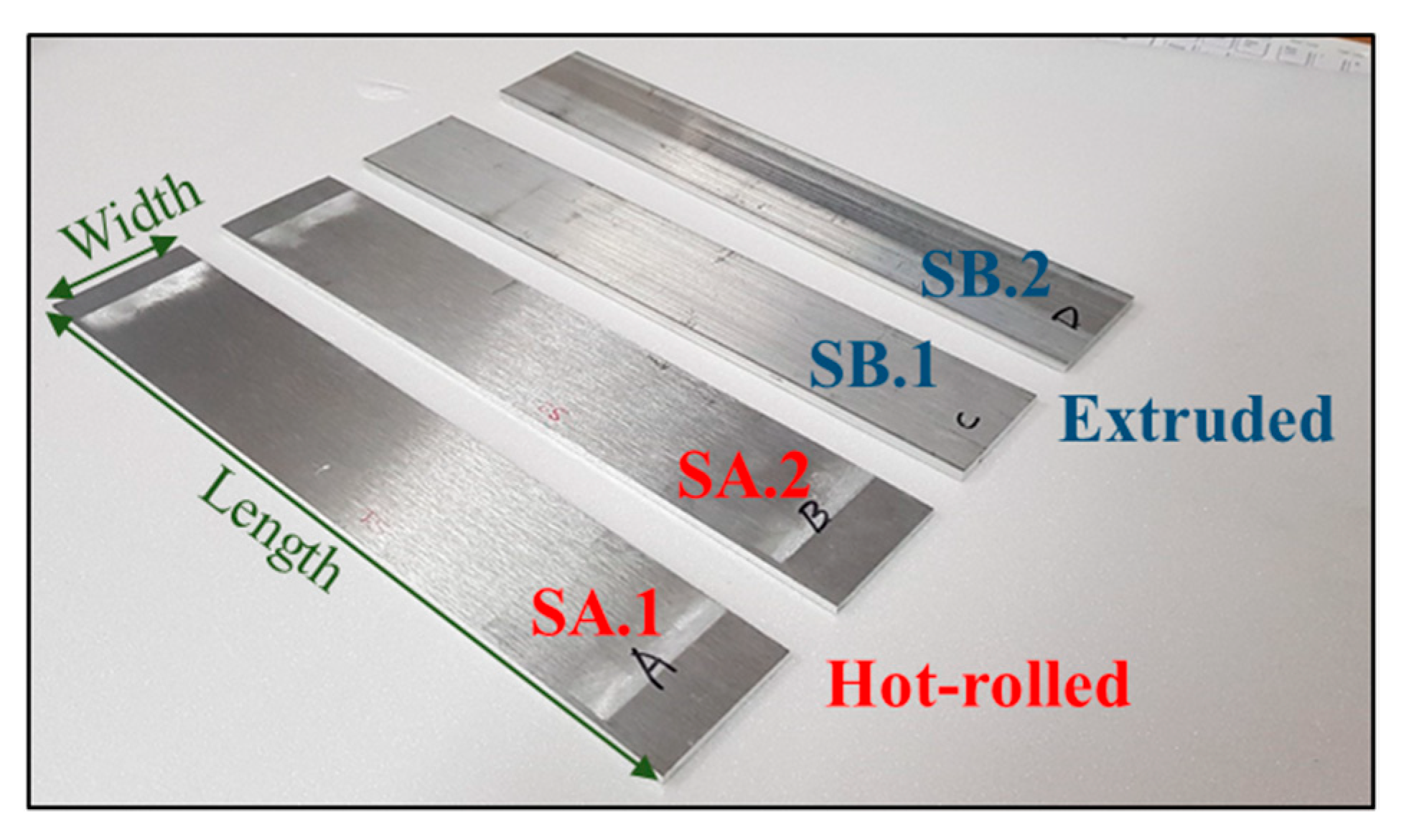
To verify the proposed method experimentally, stress estimation experiments were performed. Two kinds of Al6061 material with different acoustic anisotropy rates were used as the test specimens. One (SA) was produced by a hot rolling process and the other (SB) was produced by an extrusion process. Two test specimens were prepared for each material as shown in Figure 6. One specimen was used to check the anisotropy and acoustoelastic coefficient, and the other was used to verify the stress estimation method. The size of the hot rolled specimen is 350 mm × 62 mm × 4 mm (length × width × thickness) and the size of the extruded specimen is 350 mm × 60 mm × 5 mm.

To verify the surface wave velocity distribution and anisotropy rate of each specimen, the velocity was measured in 24 directions with an interval of 15°. The experimental setup is shown in Figure 7. PZT transducers with a center frequency of 2.25 MHz and wedges (ABWML-7T-90, Olympus) were used for surface wave excitation and reception. A pulser-receiver (Olympus 5077PR) was used for the excitation with a single pulse and a high-resolution digital oscilloscope (Lecroy HDO4034A) with a 10 GS/s sampling rate was used for precise measurement of small velocity changes. The surface wave propagation distance was fixed at 10 mm using a jig. The time of flight (TOF) was used to measure the change rate of the surface wave velocities or surface wave velocity ratios used in Equations (11)–(15). The TOF was measured based on the arrival time of the peak of the pulse signal. In addition, the delay time irrespective of surface wave propagation on the specimens, such as the delay in the wedge, was compensated by calibration in advance.

The measurement results of the surface wave velocity distribution are shown in Figure 8, in which the velocity was normalized with respect to the maximum velocity. Maximum velocity (V_max) and minimum velocity (V_min) in the hot-rolled specimen are 2967.1 m/s and 2957.5 m/s, respectively, and they are 2951.8 m/s and 2876.2 m/s, respectively, in extruded specimen. Figure 8a display the results of the hot-rolled aluminum specimen (SA.1) and Figure 8b shows the results of the extruded aluminum specimen (SB.1). The acoustic anisotropy rate of the hot-rolled aluminum specimen (SA.1) was 0.005 (0.5%) and that of the extruded aluminum specimen was 0.026 (2.6%). This demonstrates that specimen SA is nearly isotropic while specimen SB has a weak anisotropic feature.

4.2. Measurement of Acoustoelastic Coefficients

The acoustoelastic coefficients were obtained prior to the stress estimation experiments. The measurement set-up is shown in Figure 9. Based on the definition of the acoustoelastic coefficient, the change rates of the surface wave velocity were measured with stress in the stress direction (K₁) and in the perpendicular direction (K₂) in the uniaxial stress state. A tensile tester (Zwick-Roell) was used to apply the stress. The loading force was varied between 2500 N–22,500 N with an interval of 2500 N. The loading interval of 2500 N corresponds to a stress of about 10 MPa. The velocity measurement set-up is identical to the set-up described in Figure 7.

Figure 10 shows the change of the received pulsed surface wave signal according to the applied stress. Figure 10a corresponds to the K₁ measurement and Figure 10b reflects K₂. As shown in the zoomed-in box, the peak points of the pulse signal shift depend on the stress increment. That is, the surface wave velocity in the stress direction decreases with the stress increment, while it increases in the direction perpendicular to the stress.

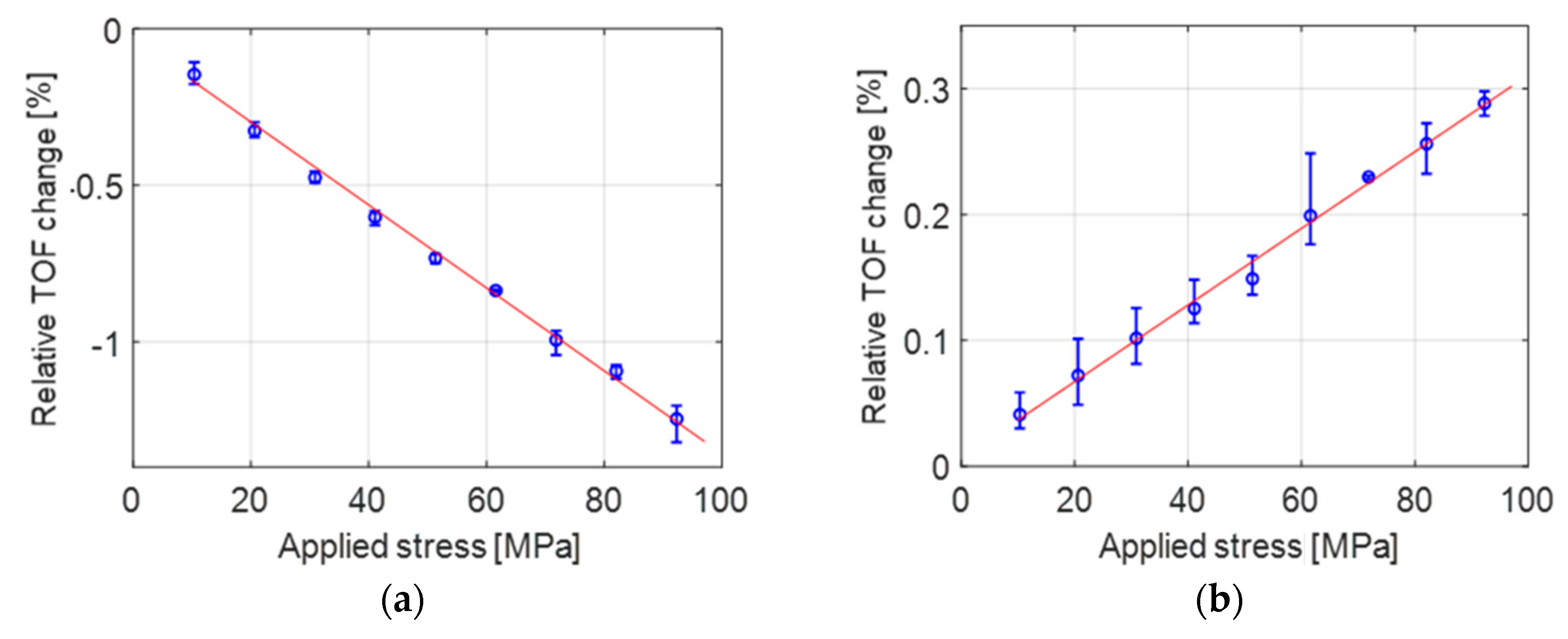
Figure 11 and Figure 12 show the change rates of the time of flight (TOF) with respect to the applied stress in each direction for the SA.1 and SB.1 specimens, respectively. The results were linearly fitted and the slopes of the fitted lines are the acoustoelastic coefficients defined in Equations (11) and (12). The obtained acoustoelastic coefficients are listed in

Table 4. Values of the acoustoelastic coefficients for specimens SA.1 and SB.1.

Specimen	K1 [1/MPa]	K2 [1/MPa]
A.1	−132.6 × 10−6	30.5 × 10−6
B.1	−124.0 × 10−6	39.7 × 10−6

.

4.3. Experiments for Stress Estimation

The stress estimation set-up is shown in Figure 13. The experimental set-up is similar to the acoustoelastic coefficient measurement except for the velocity measurement direction. The surface wave velocities were measured in three directions with difference of 45°, where the angle θ was set to 30°. This measurement condition corresponds to the Case 2B in the numerical simulation. Stress was applied by tensile loading from 7500 N to 22,500 N at an increment of 2500 N. Specimens SA.2 and SB.2 were used for the stress estimation.

The stress estimation results of the hot-rolled (SA.2 specimen) and extruded (SB.2 specimen) aluminum plates are plotted in Figure 14 and the detailed values are given in

Table 5. Estimated results and errors for the hot-rolled specimen (SA.2).

Given stress [MPa]	30.40	40.48	50.57	60.66	70.75	80.83	90.92
Estimated stress [MPa]	28.90	36.42	47.01	61.46	66.54	77.82	85.78
Stress estimated error [MPa]	1.50	4.06	3.56	−0.80	4.21	3.01	5.14
Estimated angle $\theta$[°]	23.39	25.41	26.18	25.35	20.17	26.23	27.73
Angle Estimated Error [°]	6.61	4.59	3.82	4.65	9.83	3.77	2.27

and

Table 6. Estimated results and errors for the hot-rolled specimen (SB.2).

Given stress [MPa]	24.95	33.24	41.50	49.78	58.06	66.34	74.61
Estimated stress [MPa]	21.56	33.43	42.20	48.58	53.87	61.57	69.89
Stress estimated error [MPa]	3.39	−0.19	−0.70	1.20	4.19	4.77	4.72
Estimated angle $\theta$[°]	32.96	34.02	34.94	33.03	34.98	34.58	34.30
Angle Estimated Error [°]	−2.96	−4.02	−4.94	−3.03	−4.98	−4.58	−4.30

, respectively. For the hot-rolled aluminum specimen, the estimated results match the given stresses and angle well. Similarly, the stress and angle estimations for the extruded specimens also exhibit a good agreement with the applied values even though this specimen has a larger anisotropy rate than the hot-rolled specimen. The maximum error was 5.14 MPa at a given stress of 90.92 MPa in the hot-rolled specimen, and the other errors were less than 5.00 MPa for both specimens. As a result, it was confirmed that stresses can be estimated in weakly anisotropic materials using the proposed method. Note that the experiments were carried out for the case where the stress in the thickness direction was uniform only to verify the proposed method. If the stress varies with depth, surface waves of different wavelengths can be used to probe the stress field at different depths.

5. Conclusions

This study proposed a method to estimate stress in anisotropic materials, which involved modification of the equation for the isotropic theory. In this method, the ratios of the surface wave velocities in the stressed state to those in the stress-free state in three directions were utilized, enabling simultaneous estimation of the principal stresses and their directions.

Numerical simulations and experiments were conducted for verification. The results of the numerical simulation showed that the stress estimation error occurred at a very small order when the acousitc anisotropy rate was less than 2%. Experiments were performed on hot-rolled and extruded aluminum plates that had different anisotropy rates of, 0.05% and 2.6%, respectively. The stresses applied by a tensile tester were estimated by measuring the ratios of the surface wave velocities in the stressed state to those in the unstressed state in three-directions. The estimated results showed good agreement with the given stresses in the range from 30 to 90 MPa. These results demonstrate that the stress estimation method proposed in this study can effectively estimate the stress in weakly anisotropic materials. The proposed method is simple, practical and is expected to be useful for monitoring changes in surface stress before and after machining such as punching or bending of plates.

References

- Hughes, D.S.; Kelly, J.L. Second-order elastic deformation of solids. Phys. Rev. 1953, 92, 1145. [Google Scholar] [CrossRef]
- Javadi, Y.; Plevris, V.; Najafabadi, M.A. Using LCR ultrasonic method to evaluate residual stress in dissimilar welded pipes. Int. J. Innov. Manag. Technol. 2013, 4, 170–174. [Google Scholar]
- Gokhale, S.J.T.A. Determination of Applied Stresses in Rails Using the Acoustoelastic Effect of Ultrasonic Waves. Master’s Thesis, Texas A&M University, College Station, TX, USA, 2007. [Google Scholar]
- Hughes, J.; Vidler, J.; Khanna, A.; Mohabuth, M.; Kotooussov, A.; Ng, C. Measurement of residual stresses in rails using Rayleigh waves. In Proceedings of the International Conference on Structural Integrity and Failure, Perth, Australia, 3–6 December 2018. [Google Scholar]
- Bray, D.E.; Tang, W.J.N.E. Subsurface stress evaluation in steel plates and bars using the LCR ultrasonic wave. Nucl. Eng. Des. 2001, 207, 231–240. [Google Scholar] [CrossRef]
- Jassby, K.; Saltoun, D. Use of ultrasonic Rayleigh waves for the measurement of applied biaxial surface stresses in aluminum 2024-T 351 alloy. Mater. Eval. 1982, 40, 198–205. [Google Scholar]
- Lu, W.; Peng, L.; Holland, S. Measurement of acoustoelastic effect of Rayleigh surface waves using laser ultrasonics. In Review of Progress in Quantitative Nondestructive Evaluation; Springer: Boston, MA, USA, 1998; pp. 1643–1648. [Google Scholar]
- Delsanto, P.; Clark, A.V., Jr. Rayleigh wave propagation in deformed orthotropic materials. J. Acoust. Soc. Am. 1987, 81, 952–960. [Google Scholar] [CrossRef]
- Mase, G.; Delsanto, P. Acoustoelasticity using surface waves in slightly anisotropic materials. In Review of Progress in Quantitative Nondestructive Evaluation; Springer: Boston, MA, USA, 1988; pp. 1349–1356. [Google Scholar]
- Thompson, R.B.; Lee, S.; Smith, J.F. Angular dependence of ultrasonic wave propagation in a stressed, orthorhombic continuum: Theory and application to the measurement of stress and texture. J. Acoust. Soc. Am. 1986, 80, 921–931. [Google Scholar] [CrossRef] [Green Version]
Figure 1.
Schematic of the relationships of the angles between the principal stress direction and three-measuring directions in 45° increments, in which θ is the angle from a measuring direction to the principal stress (σ1) direction, and Vθ, Vθ−45, Vθ−90 are surface wave velocities propagating in the θ, θ − 45°, and θ − 90° directions, respectively.
Figure 2.
Principal stress (σ1) direction, and three-measuring directions in 45° increments, in which θ is the angle from a measuring direction to the principal stress (σ1) direction and ϕ is the angle to the anisotropy direction, and Vθ, Vθ−45, Vθ−90 are surface wave velocities propagating in the θ, θ − 45°, and θ − 90° directions, respectively.
Figure 3.
Surface wave velocity according to the propagation direction for unstressed and stressed states in an anisotropic material.
Figure 4.
Stress estimation errors of the isotropic theory with respect to the anisotropy rate (Case 1A).
Figure 5.
Stress estimation errors of the proposed method with respect to the anisotropy rate (a) Case 1A; (b) Case 1B; (c) Case 2A; (d) Case 2B; (e) Case 3A; (f) Case 3B.
Figure 6.
Aluminum plate specimens used in experiments.
Figure 7.
Surface wave velocity measurement set-up, in which the distance fixing zig holds the wedges to keep the surface wave propagation distance constant.
Figure 8.
Surface wave velocity distributions of the two specimens: (a) Hot rolled specimen (SA.1); (b) Extruded specimen (SB.1).
Figure 9.
Set-up for acoustoelastic coefficient measurement. The change in surface wave velocity under tensile stress loading is measured. For the measurement of K1, transducers (blue colored) are placed in the loading direction, while for the measurement of K2, transducers (orange colored) are placed in the direction perpendicular to the loading direction.
Figure 10.
Received signals obtained in the acoustoelastic coefficient measurements: (a) Measurement of K1—The peak moves to the right because the velocity of surface wave in the direction of tensile stress decreases with increasing stress; (b) Measurement of K2—The peak moves to the left because the velocity of surface wave in the direction perpendicular to the tensile stress increases with increasing stress.
Figure 11.
Change rates of the TOF with respect to the applied stress in specimen SA.1 for measurements of (a) K1 and (b) K2.
Figure 12.
Change rates of the TOF with respect to the applied stress in specimen SB.1 for measurements of (a) K1 and (b) K2.
Figure 13.
Experimental set-up for the proposed stress estimation.
Figure 14.
Stress estimation results (a) Hot-rolled specimen (SA.2) and (b) Extruded specimen (SB.2).