Inducing Damage Diagnosis Capabilities in Carbon Fiber Reinforced Polymer Composites by Magnetoelastic Sensor Integration via 3D Printing

Abstract

This study investigates the possibility of inducing damage diagnosis capabilities in carbon fiber reinforced polymer composite slabs using custom-built integrated sensors and conventional, affordable equipment. The concept utilizes magnetoelastic strips integrated via 3D printing procedures in composite slabs. Under external mechanical loading, the strip magnetization changes due to the magnetoelastic phenomenon. Accordingly, electrical signals may be passively induced in conventional reception coil circuits placed at a distance from the slab. Since these signals quantify the vibrating slab’s response, which is affected by the slab’s structural integrity, damage may be detected when specific signal characteristics change. Two main issues are examined, namely the ability of receiving meaningful (with respect to noise) electrical signals from the built-in strips despite their contact-less passive reception, and the potential of diagnosing damage using such signals. Hence, slabs of various sizes and levels of structural damage (notches) have been vibrated at different frequencies and amplitudes. Treating the experimental data from integrated strips by applying the proposed processing framework allows for calculating eigenfrequencies sensitive to occurring damage (and its severity), as verified by finite element models of the vibrating slabs. Accordingly, damage may be detected and evaluated via the currently proposed experimental testing and analysis framework.

1. Introduction

In the past decade considerable advances have been made in the technology of rapid manufacturing. Not only have the techniques per se evolved, but the range of available materials for the so-called 3D printing technologies (or additive manufacturing) has also widened [1]. Numerous works in the literature already refer to the next level of meta-structures which can be designed and manufactured under the provocative term “4D printing”, referring to materials and structures with time-dependent response or geometry [2]. Another interesting feature of the wide range of additive manufacturing technologies is that sensors may be easily incorporated within the layered structure during its building phase, resulting in smart systems, i.e., objects with built-in sensing capabilities [3]. Several review articles (see [4,5] for typical examples) classify such smart systems according to their manufacturing process, operating principle, and/or functionality. Different types of sensors, e.g., optical for interactive devices [6], or embedded wires for capacitive sensing applications [7,8] have been suggested as potential smart systems. Mechanical strain sensing via various incorporated sensors in 3D printed systems has also been proposed [9,10,11]. Magnetite/thermoplastic composite in 3D printing as direct replacements for commercially available flow sensors [12], or custom-built devices (whiskers) with built-in magnetostrictive materials for specific flow measuring applications [13] have been successfully manufactured. Magnetic force sensors [14], or devices for sensing human tactile force and imperceptible skin deformation due to heart pulses [15] for biomechanical applications are reported as feasible options for 3D printed smart objects. Specifically, some applications related to stretchable sensors for biomedical purposes are also reported in [16].

On the other hand, several custom-built sensors designed to monitor structures for damage diagnosis purposes, have been proposed over the recent years, for instance [17,18,19,20,21,22]. Such sensors are mostly designed to be patched onto the structure, so that the sensing element such as, fiber bragg gratings [18,19], magnetoelastic strips [21], and PZT impedance [22] or MFC (macro-fiber composite) transducers [23] to name but a few, could measure specific dynamic properties of the structure under vibration.

Magnetoelastic sensors have been under intense investigation for many applications in the past decade. Since they react to changes in imposed mechanical strain, by changing their magnetic constant, they can be used as wireless and passive sensors at the same time. Magnetoelastic sensors are usually made by rapid melt quenching, in the form of amorphous ferromagnetic ribbons. Most members of this family are iron-rich alloys, such as the well-known Fe₄₀Ni₃₈Mo₄B₁₈ marketed under the commercial name Metglas^®2826 MB. The authors have successfully used this material as a damage sensor for polymers and composite systems [21] and have gathered considerable experience in sensor application, data gathering, and processing over the last years. A main advantage of such sensors against all other types of relevant devices is that they require no wiring, electrical nor optical, and can be interrogated wirelessly and in a passive state.

In general, the sensor is carefully configured in order to interfere as little as possible with the monitored structure’s dynamics. Therefore, the sensor weight and volume are kept as low as possible, meaning that in some cases even thermal-spraying techniques to achieve deposition of sensing element (copper electrodes) onto the structure [24] may be used. A notable exception to this rule is found in [25], where the sensor placed on the structure is deliberately chosen of considerable weight so as to change at will the underlying dynamics.

In general, 3D printing procedures have been used for the sensor’s construction [17] or the integration of the necessary circuitry/devices in order to facilitate operation of laser displacement sensors [20] or MFC sensors/transducers [23]. In other words, the 3D printing process has very often served as a means of facilitating the sensor’s construction process, or it’s mounting onto a given structure and its effective operation, but it has rarely been used for manufacturing a structure with a sensing element integrated within.

The aim of the current study is to use the additive manufacturing principle for integrating sensing elements in a structure during its 3D printing process, and to diagnose structural damage based on data from these built-in sensing elements and conventional, affordable equipment. The considered structures are carbon fiber reinforced polymer (CFRP) composite slabs of different dimensions, which incorporate magnetoelastic strips acting as sensing elements under external slab loading. Then, due to the magnetoelastic phenomenon, such loading lead to changes in the strip’s magnetization, which causes the induction of electrical signals in conventional reception coil circuits placed at a distance from the slab. Since these signals quantify the vibrating slab’s response (itself depending on the slab’s structural integrity) damage is detectable when changes of specific signal characteristics (selected eigenfrequencies) occur. Even if, at times, this detection principle may prove not very practical to use, it is a traditional approach for structural health monitoring purposes, as it can be sensitive to even small damages [25].

This detection principle has also been used in a recent study [26], which features a similar operational and testing concept to that proposed in the current work, but for the important detail of the magnetoelastic sensing material being attached onto (rather than integrated within) the structure. Due to this critical difference, two main issues must be dealt with, namely the possibility of recording meaningful (with respect to noise) electrical signals from the built-in strips despite their contact-less reception, and the potential of diagnosing damage using such signals. Therefore, slabs of various dimensions and damage levels have been vibrated at different frequencies and amplitudes. Via a dedicated test data processing framework along with finite element method (FEM) analysis, it is shown that magnetoelastic strips integrated within the material structure may successfully act as passive embedded sensors, transmitting meaningful signals during mechanical loading and providing qualitative and quantitative damage diagnosis results.

The rest of the paper is organized as follows: Section 2 presents the 3D printing process of CFRP slabs with the integration of sensing elements, and the testing protocol used for the experiments. In Section 3, the experimental data along with the relevant framework for data analysis and validation via FEM are shown. Based on this framework, damage detection and assessment results are obtained and commented upon. Finally, Section 4 presents some concluding remarks.

2. Materials and Methods

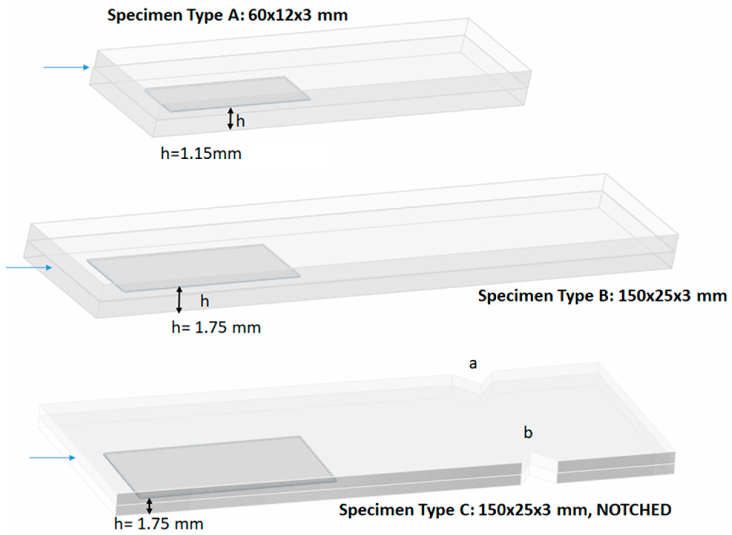
2.1. Slab Preparation by 3D Printing

A reprap project series clone model of a 3D printer (CTC i3, Zhuhai Electronic Ltd, Zhuhai City, Guangdong, China) operated by an Arduino^® controller, was used to prepare the slabs. The printer operated in Fused Deposition Modeling (FDM) mode, had a single nozzle (diameter of 0.4 mm) and used a 1.75 mm polymer filament. The filament was a short carbon fiber reinforced PET-G polymer composite by 20 wt% (NEEMA3D™ Carbon: plus) of NEEMA3D™, Petroupolis, Greece. The filament had a Young’s modulus of E = 3800 MPa and a yield strength of 52.5 MPa according to the manufacturer’s specifications.

Rectangular slabs of 60 × 12 × 3 mm³ (hereafter referred to as type-A slabs) were prepared by means of the FDM printer, which was paused once the desired layer height was reached, so as to allow for attaching the 2826 MB Metglas^® magnetoelastic (20 μm) strip of 25 × 5 mm² (kindly donated by Prof. D. Kouzoudis, University of Patras). The magnetoelastic strips were attached to the desired depth by means of an epoxy adhesive. Subsequently, the magnetoelastic strip was covered by successive material layers until obtaining the final slab thickness (Figure 1). In this way, one set of type-A slabs with “hidden” built-in magnetoelastic strip sensors, hereafter referred to as M-sensors, was prepared. Again, another series of type-A slabs without magnetoelastic strips (type-A blanc) was also prepared for testing purposes.

Two sets of larger slabs of 150 × 25 × 3 mm³ were also prepared for the testing and may be seen in Figure 2. As seen in Figure 2, the magnetoelastic strip was placed inside the specimens during the 3D printing procedure, at heights of h = 1.15 mm for specimen’s type A and h = 1.75 mm for specimen Types B and C, with respect to the specimen’s total thickness, measuring from the bottom of the slabs.

The first set involved M-sensor slabs (hereafter referred to as type-B slabs) and the series contained artificially damaged M-sensor slabs with one or two transverse notches (hereafter referred to as type-C1 or -C2 slabs, respectively), made with a diamond saw and featuring a depth of 1.5 mm.

Not that preparing two different slab sizes (type-A and type-B/-C1/-C2) was necessary because of technical limitations imposed by the testing procedures, as explained in the next subsection. Details on the objectives to be achieved and the testing protocol are given in the following subsection.

2.2. Experimental Procedures

Successful M-sensor operation depends on achieving two objectives:

• O1: That meaningful (with respect to noise) electrical signals passively emitted from M-sensors could be generated/recorded, and
• O2: That the analysis of recorded signals could provide damage detection and assessment (diagnosis) results, especially at high amplitude/low frequency vibrating operation.

The reason for focusing on high amplitude/low frequency operation in O2 is because both objectives were achieved in a high frequency/low amplitude vibrating context [21], even though the magnetoelastic strip was attached on the surface of the vibrating slab. Nonetheless, objective O1 was checked under all frequency—amplitude combinations, simply to ensure that the slabs with built-in strips do operate as sensors under such conditions. Two testing procedures have been used for checking whether O1 and O2 were achievable:

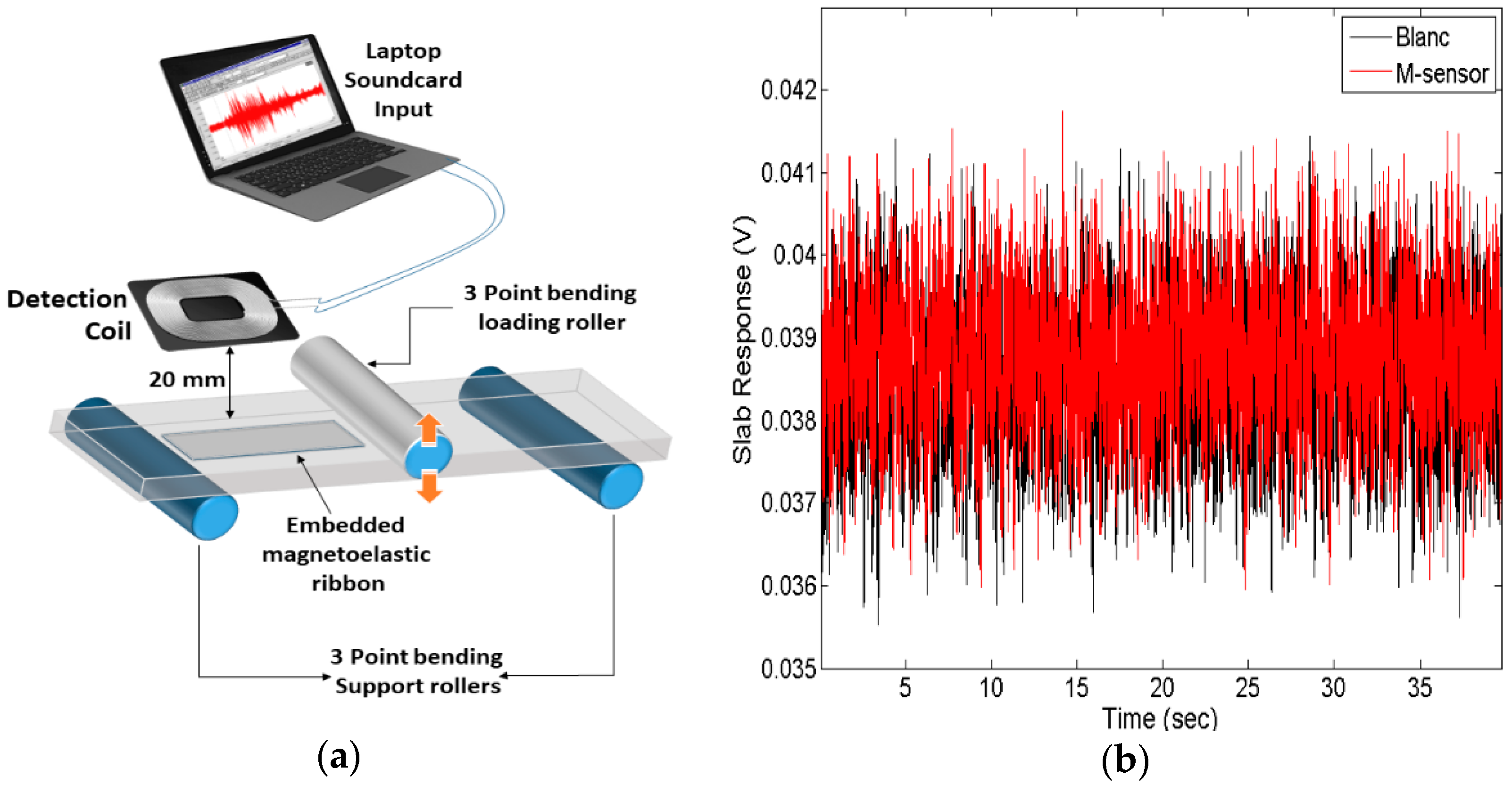
• P1: The procedure simulated high frequency and low amplitude operational conditions, typical of systems with fast dynamics and involved type-A slabs both in M-sensor and blanc (type-A blanc) forms. Testing was performed on a Dynamic Mechanical Analyzer (DMA Q800) of TA—Instruments (Figure 3), which led to choosing the specific dimensions of type-A slabs. Slabs were subjected to three-point dynamic bending under a linear frequency scan of 1–100 Hz @ RT and at v = 25 μm constant static deflection. Electrical signals created by induction to the remote interrogation coil (placed at 20 mm from the slab) were recorded by PioneerHill-Spectraplus© Software for Data Acquisition at 4096 Hz via a PC-Soundcard 3.5 mm jack. Comparing signals from type-A and -A blanc slabs allows for validating whether the hidden magnetoelastic material could provide sensing capabilities to the (otherwise passive) slab.
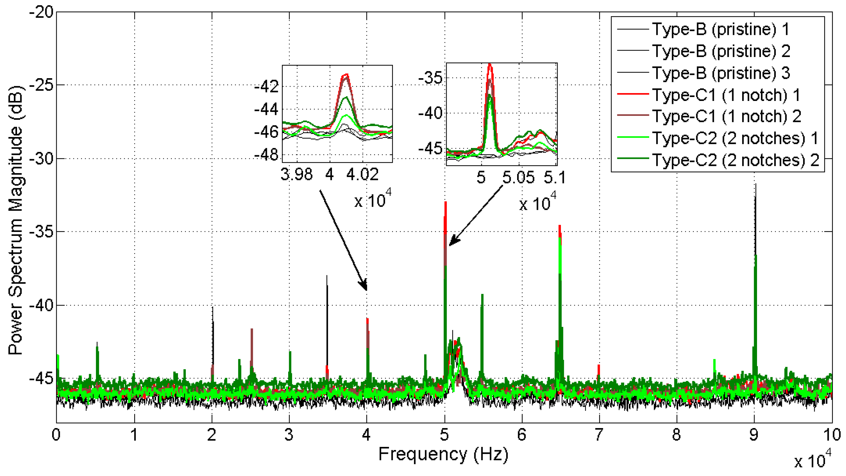
• P2: The procedure involved series of type-B and -C1, -C2 slabs, fixed as cantilevers (Figure 4). The free end suffered a load of quasi-sinusoidal form with frequency f = 4 Hz, mean value equal to 12.5 mm and amplitude d = 12.5 mm. In other words, the free end featured deflections between 0 and 25 mm, applied via a custom-built mechanical exciter, which allowed for using a (larger than type-A) size of type-B/-C1/-C2 slabs. Hence, low frequency and high amplitude operational conditions typical of systems (structures) with slow dynamics were simulated. Electrical signals created by induction to a low-cost interrogation coil (Vishay IWAS) placed at 20 mm from the vibrating slab’s end, were recorded via a conventional digital oscilloscope at 200 KHz. C comparing signals from pristine (type-B) or damaged (-C1, -C2) slabs should conclude on the existence of frequency shifts and ensure that damage diagnosis results could be obtained using the M-sensor concept.

Note that the coil distance of 20 mm from the slab was defined by a trial-and-error process, and corresponds to the maximum distance for recording a meaningful signal with the given set up. Obviously, placing the coil very close (or onto) the surface should provide better signal recording capabilities, but it would undermine the practical aspects of the concept and could induce sensitivity to the “lift-off” effects noted, for instance, in applications based on Eddy currents. All recorded signals were analyzed with respect to their power spectra, estimated via the Welch method (usually coded in various software packages such as MATLAB^®) with results presented in Section 3.

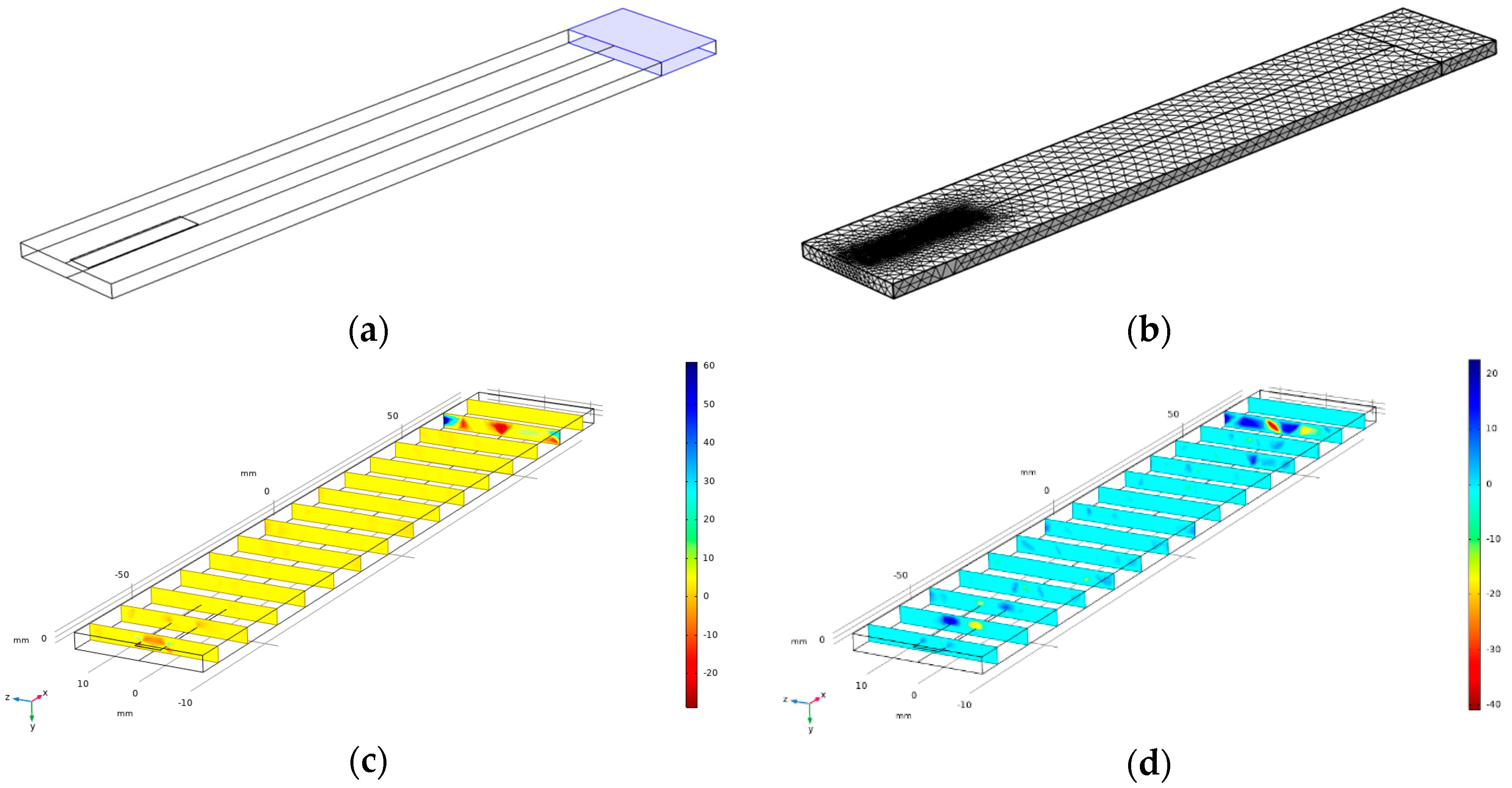
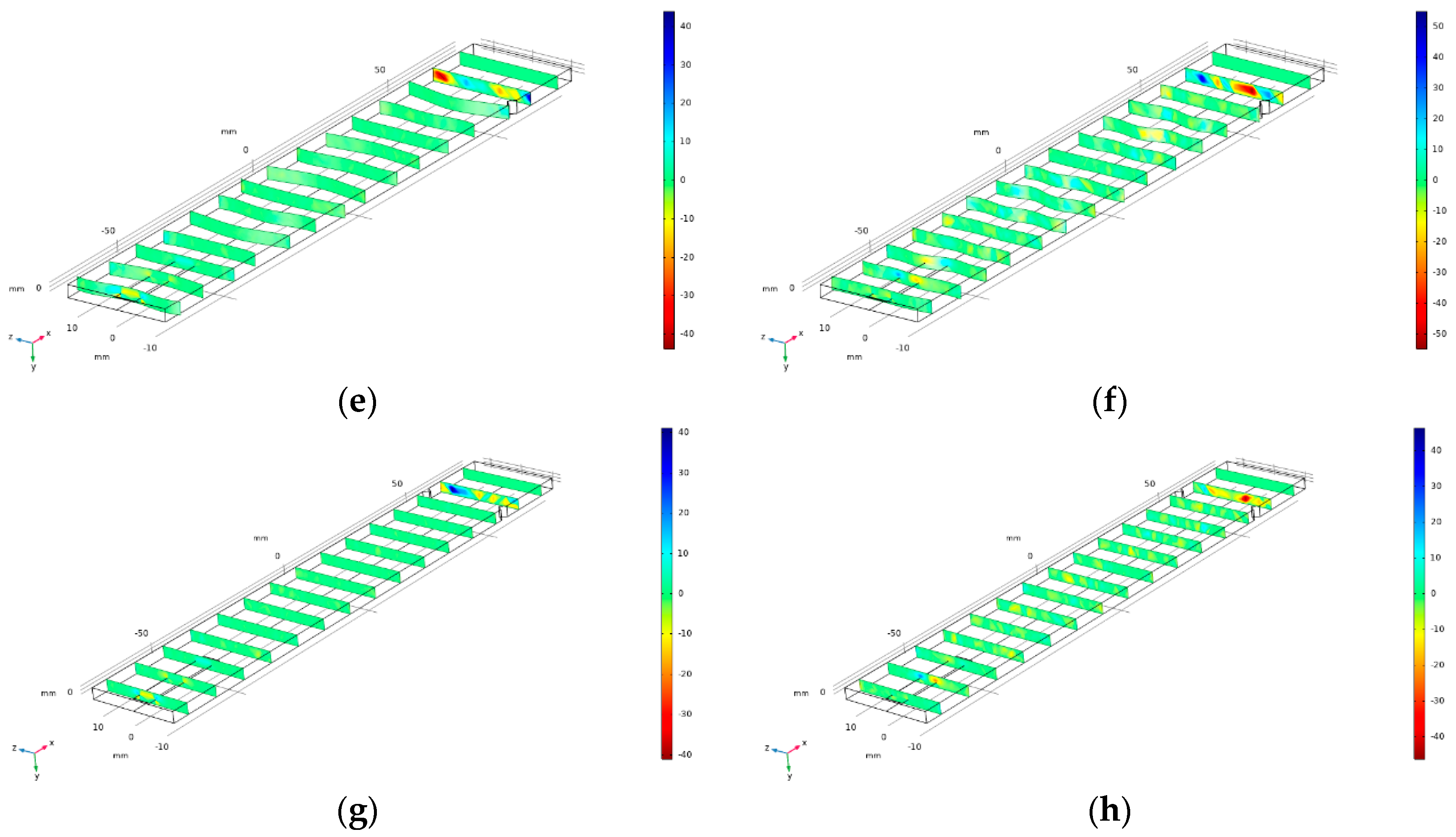
2.3. Finite Element Method Analysis

For achieving objective O2, the eigenfrequencies of type-B, -C1 and -C2 slabs involved in testing should be experimentally computed, and compared to their corresponding theoretical values. The latter were computed via FEM analysis, thus enabling to model and study complete type-B, -C1 and -C2 slabs, meaning that the magnetoelastic sensor (type-B), or even notches (-C1 and -C2 slabs) were incorporated. FEM COMSOL Multiphysics 5.4 software was used to model the process and compute the eigenfrequencies and mode shapes of the cantilever slabs with point loading (see Section 3.2). Free tetrahedral and boundary triangular elements were selected for meshing. Mesh size was selected as finer, because extremely finer meshes did not have a significant effect on the results. The required number of elements for meshing was found equal to 166.301 in total, while minimum element quality was set to 0.05. In all cases, the computations employed second-order polynomials.

3. Experimental Results and Analysis

3.1. Testing for Meaningful Signals with Respect to Noise (O1)

As described in Section 2.2, the DMA testing provided a conventional, yet rigorous means of testing whether the objective O1 is achievable. The procedure P1 involved a relatively high vibration frequency peak of 100 Hz and low vibration amplitude of 25 μm defined in the DMA operational settings. Two type-A blanc and two -A slabs were initially tested in dynamic three-point bending see Figure 3a. Typical responses of one type-A and one -A blanc in form of electrical signals (in V) versus time are presented in Figure 3b. Obviously, based on the time plot alone, no quantitative distinction (for instance, differences on signal variance or mean) between signals from type-A and -A blanc slabs may be noted. This behavior is not unreasonable, because the external mechanical loading cannot generate significant electrical power by means of the magnetoelastic phenomenon. Consequently, when similar passive techniques (i.e., no excitation on the reception coil) are utilized, one should at best expect qualitative rather than quantitative changes in the signals recorded. In other words, the spectral characteristics of such signals should be analyzed.

Figure 5 presents the power spectra corresponding to response signals from two type-A blanc and two A slabs showing clear differences. The insets show significant spikes at around 740 and 1220 Hz for signals from the two type-A slabs (red and green lines, respectively). At these frequencies, at least, there is a visible contribution from the M-sensor, superseding the effects of other phenomena (noise and so on). The latter show up as an output response signal on the coil even when a type-A blanc slab is tested.

Furthermore, in view of Figure 5, note that the slab excitation takes place at frequencies up to 100 Hz, yet the slab response shows mainly frequency content (harmonics) at higher frequencies (740 and 1220 Hz). The explanation may be two-fold. First, Figure 5 suggests that, at low frequencies (up to 200 Hz), a type-A slab actually produces a signal which has insignificant frequency content, barely distinguishable from parasitic noise. At higher frequencies and especially at 740, 1220 Hz, or more, the magnetoelastic strip seems to be generating a signal with more significant frequency content. This lack of sensitivity might be alleviated if a more efficient (and, thus, expensive) coil was used, but this would compromise one of the main goals of this work, namely performing damage diagnosis via conventional, affordable solutions. Second, there is the possibility of the vibrating slab behaving in a nonlinear manner. External loading of the slab at a given frequency produces a response signal with a shift of that frequency (and its harmonics), see Ch. 5 in [27]. Even though it is not trivial to state which explanation is valid, the fact is that, at a specific frequency band, the M-sensor can provide a signal qualitatively different than that recorded by vibrating type–A blanc slabs, thus achieving objective O1.

3.2. Testing for Damage Detection Capabilities (O2)

Section 2.2 described the second objective (O2) which should be achieved by following the testing procedure P2, namely that of obtaining signals useful for detecting and assessing (diagnosing) damage in the corresponding slabs, especially for vibrations of low frequency and high amplitude.

Procedure P2 was applied to three type-B slabs (pristine condition), two type-C1 slabs (thus, involving one notch), and two more -C2 slabs (with two notches-see Figure 2). Testing involved vibrating the free slab end at 4 Hz, with mean value of 12.5 mm and amplitude of 25 mm, with the response signals (as generated by the reception coil) recorded at 200 KHz via a conventional oscilloscope. Even though the sampling frequency is larger than those used in traditional structural monitoring systems, it is by no means unobtainable, since no particular exotic equipment solutions are needed.

Figure 6 shows the power spectra of the signal responses from the type-B slabs, with insets presenting frequency regions with the largest spikes from test data of at least two out of the three type-B slabs tested. From tests with type-A (see Section 3.1), it was deduced that an M-sensor slab provides meaningful signal (with respect to its frequency content) at high frequencies. At the same time, a convenient fact is that small damage may be quite clearly indicated at higher modes of vibration [25]. Hence, one should check whether the spikes noted in Figure 6 actually correspond to eigenfrequencies, so that they could be used for damage diagnosis purposes. Therefore, the FEM analysis described in Section 2.3 was carried out.

Figure 7 presents indicative results of type-B, -C1 and -C2 slabs for two frequency ranges (around 47,000 and 90,000 Hz). These plots resulted from the finite elements modal vibration analysis and show the eigenfrequencies and eigenmodes of the combined structure (slab and ribbon) at two significant frequencies noted in signal power spectral analysis (Figure 6). As seen, type-B slabs show quite different behavior to that of type-C1, -C2 slabs for both frequency bands. The results from eigenfrequencies determination for a type-B (among others) slab are presented in

Table 1. Eigenfrequencies of type-B, -C1 and -C2 slabs as determined by the solution of the finite elements model compared with the ones picked up in signal power spectra.

FEM Eigenfrequencies in Hz for Indicated Slab: (I)			Power Spectra Eigenfrequencies in Hz for Indicated Slab: (II)			Absolute Value of % Error: abs{(I)-(II)}/(I)
-B	-C1	-C2	-B	-C1	-C2	-B	-C1	-C2
4982.4	4986.9	5158.5	5235	5230	5233	5	5	1.4
20,389	20,373	19,985	20,142	20,140	20,140	1.2	1.1	0.8
34,804	34,798	35,257	34,868	34,865	34,868	0.2	0.2	1.1
47,402	47,253	47,017	47,553	47,555	47,555	0.3	0.6	1.1
65,038	65,007	65,061	64,898	64,900	64,895	0.2	0.2	0.3
89,994	90,038	90,064	90,135	90,133	90,133	0.2	0.2	0.1

and compared with those resulting from Figure 6, whereas their percent error is also shown. Interestingly, the six largest spikes in Figure 6 are at frequency values extremely close to the eigenfrequencies of type-B slabs. The percent error shown in Table 1 is almost insignificant, except for the lowest eigenfrequency at 4982.4 Hz, where it reaches almost 5%. This is in agreement with findings of type-A slab testing (Section 3.1), where the M-sensor’s output frequency content was significant mainly at higher frequencies. So, finite element modal analysis has confirmed the values of significant eigenfrequencies of the specimens as detected in the experimentally obtained signals.

This result could be anticipated, even without the FEM analysis. In fact, every realistic implementation of a quasi-sinusoidal excitation would trigger harmonics in the response signal, with their magnitude in the signal power spectrum following a decreasing trend with growing frequency values. On the rare occasion of spikes actually becoming larger with growing frequencies, one may start thinking of such harmonics being close to eigenfrequencies of the tested structure.

Figure 8 shows the power spectra of the signal responses from two type-C1 and another two type-C2 slabs. Power spectra of signals from type-B slabs are also presented for comparison. Considering the 6 largest spikes (as for the case of test data from type-B slabs), it results that type-C1 and -C2 slabs show spikes at approximately the same frequencies as type-B slabs (see Table 1) except for the spikes at 50,110 Hz and 40,090 Hz.

These values were also cross-validated via FEM analysis: Eigenfrequencies at the region of 50 KHz were computed at 49,545 Hz and 49,946 Hz for -C1 and -C2 slabs, respectively. Again, as observed at the region of 40 KHz, eigenfrequencies equal to 39,936 Hz and 40,088 Hz were computed for -C1 and -C2 slabs, respectively. In all cases, the percent errors of the experimentally obtained (via power spectra) eigenfrequency values with respect to those computed via FEM analysis are extremely small. In both cases, the spike occurrences indicate alterations in structural condition, because at these frequencies no significant content was present in signals from pristine slabs (see also Figure 6). Note that in many other (mainly lower) frequency areas, one may find circumstantial evidence of spikes associated to signals from some but not all damaged slabs, in some cases somewhat undermined by noise. Hence, such frequency areas have been systematically disregarded, in favor of frequency bands where a selected number of the most prominent spikes may be clearly denoted.

There is also evidence that the damage level (one or two notches) may lead to spikes of different amplitude, since at both frequency ranges of interest (around 40 and 50 kHz), -C1 slabs feature power spectra with larger spikes than those from -C2 slabs. The analysis in [28] (specifically in Ch. 10), proposes an estimation of the damping coefficient from such plots, by associating spikes of narrower angle (i.e., more abrupt) to lower damping for a given frequency.

The fact that, at both frequencies, the spikes from -C1 slabs (in red and dark red) have a slightly narrower angle than those from -C2 slabs (in green and dark green) may indicate that damping slightly increases with notches, as should theoretically be the case [25].

Hence, damage is definitely detectable by considering a number of the most prominent spikes of the tested slab (mainly at higher frequencies) and comparing with the corresponding group of spikes from pristine slabs. Currently, frequencies around 40 and 50 KHz seem suitable for detecting damage, with occurrence of new spikes pointing to structural alteration (notches) of the tested slabs.

3.3. Testing for Damage Assessment (O2)

Even though detecting damage (notch) occurrence based on signals from testing with procedure P2 is definitely feasible, assessing the different damage levels is less trivial. Recall that damage detection proved possible at two frequency regions (40 and 50 KHz- see Section 3.2). At these regions, spikes from signals associated to -C1 and -C2 slabs differ only slightly. For an answer as to whether damage level (one or two notches) may be assessed via P2, a final series of tests has been carried out. Four -C1 and another four -C2 slabs were tested following P2 and the associated power spectra were plotted in Figure 9. Since four slabs of each damage level are available, ranges of spectrum magnitudes at 40 and 50 KHz for both damage levels may be formed. These ranges indicate the variation of spectral magnitude for signals associated to slabs with one or two notches.

At both frequencies, an obvious trend for signals from more damaged (-C2) slabs having spectra of lower magnitude than their counterparts from less damaged (-C1) slabs is obvious. Spectra from -C1 slabs range between −35.5 to −40.5 dB at 40 KHz and −26 to −32.5 dB at 50 KHz. Spectra from -C2 slabs range between −40 to −43 dB at 40 KHz and −32 to −36.5 dB at 50 KHz. In both frequency areas, there is one -C1 slab whose magnitude overlaps that corresponding to a -C2 slab. Hence, since most of -C1 slabs have spectra of larger magnitude than those from -C2, procedure P2 provides indicative (rather than definitive) answers on the damage level of the tested slab.

These conclusions are based on the (rather empirical) estimation of the magnitude of damping values at each frequency found in [28]. Various approaches (for instance using dedicated equipment to analyze mode shape) may help to characterize differences induced by the damage level to the slab vibration modes. In the current study, quantitative damping data have been obtained by the recorded signals by investing effort in signal modeling procedures, as follows:

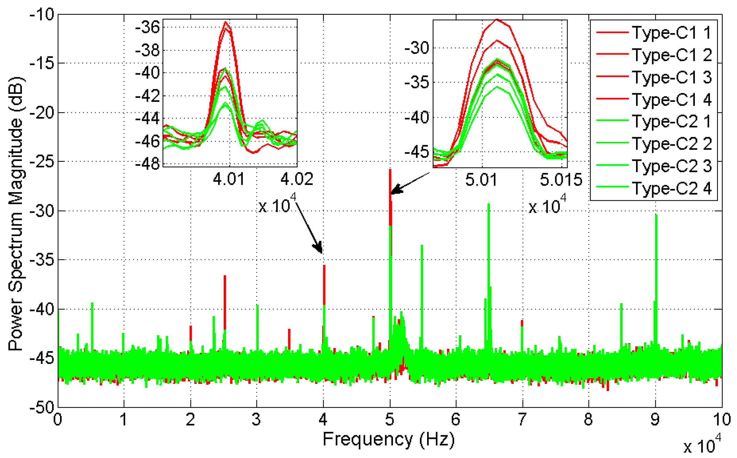
• Response signals recorded by testing each -C1 or -C2 slab using procedure P2 were treated as stochastic time-series sequences. This was quite realistic, since the recorded signals had considerable noise due to electromagnetic parasitic phenomena related to the contact-less recording principle. Furthermore, given that damage may be assessed by means of two frequency regions (around 40,000 and 50,000 Hz), it was beneficial to perform high-pass filtering of the raw signals, allowing for a lower number of frequency components to be modeled. One simple means of doing so, was by differencing the raw signals (that is, forming the differences of each signal value at instant t minus that at t − 1 for all t) as many times as necessary for effectively undermining lower frequency (below 40 KHz) components. Naturally, a traditional high pass filter may also be applied. Here, the raw signals recorded from testing with -C1 and -C2 slabs (with their spectral characteristics shown in Figure 9) were differenced six times, for obtaining signals with insignificant frequency content below 40 KHz.
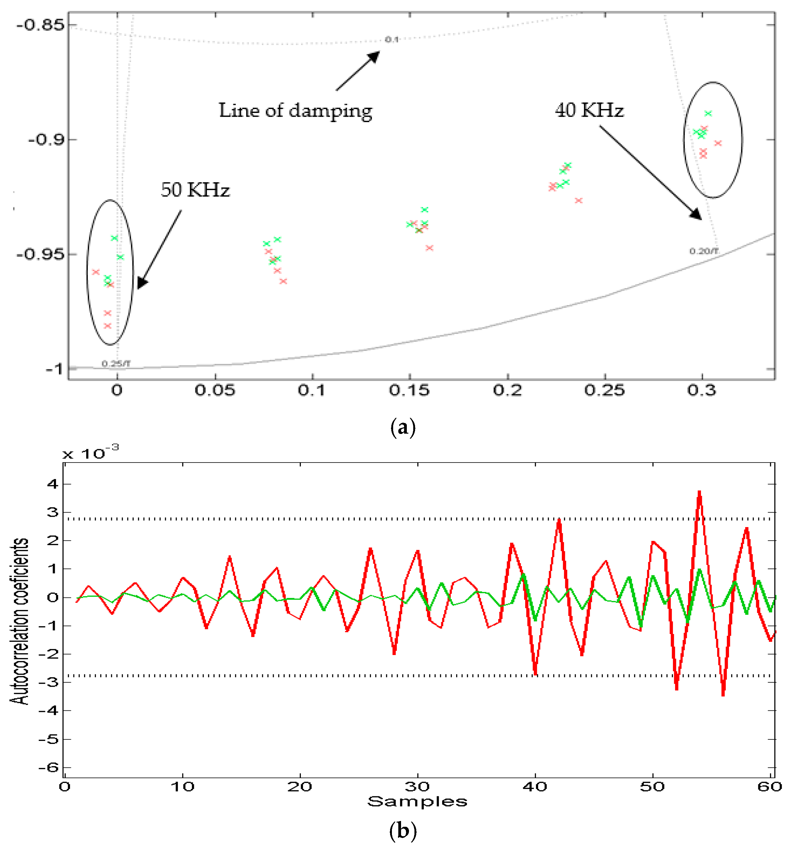
• Each signal was modeled by means of stochastic output–only AutoRegressive representations with constant coefficients (CC-AR), identified via standard algorithms. These may be coded in various programming languages, or even be found in software packages such as MATLAB^®.
• For each identified AR representation, poles at 40 and 50 KHz were monitored with respect to their damping. Characteristic changes in damping values (at these frequencies) between different data sets lead to damage assessment conclusions about the slabs generating these data.

The CC-AR representation is a standard yet effective means of modeling dependencies among values of a stochastic sequence. The stochastic output-only CC-AR representation relating the current (at time instant t) value of the modeled output signal to older ones has the following generic form:

$$\begin{array}{l}y\left[t\right]={\displaystyle {\displaystyle \sum }_{i=1}^L}{\theta }_i·p_i\left[t\right]+e\left[t\right]\\ e\left[t\right]~NID\left(0,{\sigma }_e^2\right)\end{array}$$

(1)

with t designating the normalized discrete time and y[t], e[t] the output and one-step-ahead prediction error [or residual, assumed to be a zero-mean uncorrelated sequence with variance ${\sigma }_e^2$ signals, respectively. The term NID(μ,${\sigma }_e^2$) stands for Normally Independently Distributed (with the indicated mean μ and variance ${\sigma }_e^2$). The terms p_i[t] are referred to as regressors and involve lagged output values ranging from y[t − 1] up to y[t − ny], with ny designating the maximum value of lags admitted for the signal y[t] in (1) (model order). The i-th regressor coefficient is noted θ_i and has constant value. For instance, a CC-AR representation designated as y[t] = 0.3⋅y[t − 1] + 0.7⋅y[t − 2] − 0.1⋅y[t − 3] + e[t] has an order ny equal to 3 and is usually referred to as a CC-AR(3) model. Its regressor coefficients are θ₁ = 0.3, θ₂ = 0.7 and θ₃ = −0.1.

The objective is to identify the CC-AR representation, that is, to select the regressors p_i[t] and to estimate the associated coefficients θ_i in order to most effectively represent the dynamics of the considered signal. The identification of CC-AR representation along with the estimation of coefficients θ_i are trivial procedures extensively presented in, among others, [21]. The interested reader may refer to this work for details on determining the model order and estimating the coefficients. Briefly, a signal is effectively modeled by a CC-AR(ny) representation if one determines the lowest ny value for which the associated CC-AR(ny) model accurately describes the frequency content of the signal (by assigning poles at those frequencies) and the residual sequence e[t] is uncorrelated. The latter means that the values of e[t] for various t feature insignificant mutual dependencies, as checked by specific hypothesis tests [21].

At this point, note that identifying models for fault diagnosis applications is a somewhat different task than performing identification for purposes such as control, signal pre-whitening and so on. For fault diagnosis, the identified model should include poles with frequencies as close as possible to the peak locations (frequencies) of interest in the power spectrum plot. At the same time, the identified CC-AR(ny) model should have as few regressors as possible: Extra regressors (over-modeling) may lead to fewer correlated residuals e[t] but tend to assign poles even at frequency spikes corresponding to noise or other parasitic phenomena. Over-modeling should, thus, be avoided, as far as possible.

In the current case, these peaks of interest were located at 40 and 50 KHz. Ideally, the user should determine the value range for ny, for which all associated identified CC-AR(ny) models include poles at the desired frequency peaks. In other words, one should plot CC-AR(ny) poles at each frequency as a function of the corresponding value for ny (stabilization plot), and select a value range for ny leading to obtaining poles at the desired frequency regions. At the same time, these CC-AR(ny) models should produce residuals as uncorrelated as possible. Ideally, the model structure selected should have the smallest ny of those in the range, thus avoiding any over-modeling issues.

In Figure 10a typical stabilization plot from a type-C1 test data and another from a type-C2 slabs are shown. The considered values for ny ranged from 4 up to 180. With data from either -C1 or -C2 slabs, for ny ≥ 80 the associated CC-AR(ny) models consistently assign poles at frequencies around 40 and 50 KHz. This means that for a given ny satisfying the condition ny ≥ 80, there is always a set of poles assigned to frequencies close to 40 KHz and another set for those close to 50 KHz. Hence, for the selected value of ny, the relative difference of pole damping values at each frequency may provide quantitative information on the damage level, exactly as when the power spectra of test signals are (qualitatively) examined.

Four such models have been identified on data from type -C1 slabs. Another four CC-AR(80) models have been identified on data from -C2 slabs. As shown in Figure 11a, all eight models feature poles located at the frequency band of interest (around 40 and 50 KHz). The autocorrelation coefficients of CC-AR(80) residuals computed with test data from one -C1 and one -C2 slabs (with an indicative case shown in Figure 11b) appear uncorrelated, since they are located in-between the dashed lines designating statistical limits at the 5% risk level (see [21]). Then, clearly a CC-AR(80) representation is an adequate compromise for modeling test data from -C1 and -C2 slabs.

The pole-zero maps of these eight CC-AR(80) models in Figure 11a show that at 40 and 50 KHz there is one group of four poles associated to models identified on data from -C1 slabs (red crosses) which slightly overlaps another group of four poles associated to -C2 slabs (green crosses). It is, thus, obvious that it is not possible to completely distinguish between the two groups, due to the small overlap.

However, it is also obvious that the poles associated to -C2 slabs (green crosses) have larger damping than that from poles associated to -C1 slabs (red crosses). This stems from the fact that the green crosses are closer to the dashed damping line (designating region of poles with damping coefficient equal to 0.1) than the red ones. In fact, damping of poles at 40 KHz ranges from 0.0389 to 0.0458 for -C1 slabs and from 0.0436 to 0.0508 for -C2 slabs. Damping of poles at 50 KHz ranges from 0.012 to 0.0272 for -C1 slabs and from 0.024 to 0.037 for -C2 slabs. These conclusions are identical to those resulting from the analysis based on the power spectral magnitude plots, presented above.

Moreover, tests with ny values up to 130 were also attempted only to find that, even for such high values of ny, the values in the damping of poles corresponding to -C1 and -C2 data respected the same relative order. Poles from -C1 consistently featured higher damping than those from -C2 slabs. Hence, if the relative order in damping values of poles resulting from slabs with different damage is monitored, then procedure P2 is able to provide quantitative indications about the level of damage in the tested slabs. Accordingly, the objective O2 was deemed as achievable, if only partly with respect to damage assessment. It is expected that fine-tuning P2 (or dropping the affordability condition by investing in high-tech equipment) should lead to smaller amplitude ranges for the power spectra of signals, thus achieving easier distinction of damage levels.

4. Conclusions

This study proposed a methodology for manufacturing smart slabs with embedded magnetoelastic sensors aiming at providing damage diagnosis capabilities with conventional, affordable equipment. Successful application of the proposed damage diagnosis concept requires that the smart slab must be under continuous monitoring, with the latter starting for a slab in perfect operational condition. Comparisons of experimental data over time will then detect and evaluate any occurring damage. The concept considered magnetoelastic strips integrated via 3D printing procedures in CFRP slabs. During the two testing procedures proposed, the smart slabs emitted (in a passive manner) electrical signals under vibration loading. These signals were received in a contact-less manner by conventional low-cost reception coils. The analysis of the power spectra of these signals validated the sensing concept, since they allow for computing the slab eigenfrequencies at high frequency regions. Such frequencies may thus be monitorable by combining conventional oscilloscopes, low-cost coils along with extensive analysis of the signal involved. Furthermore, it was shown that damage occurrence in slabs caused spikes in specific (high) frequency areas of the signals, and that following a specific signal modeling procedure, quantitative indications for assessing damage severity could also be found. Future work is underway to extend the concept from the current basic state (of a cantilever setup suffering from notches) to damage diagnosis cases of actual structural components. These include specimens of larger dimensions, implemented in representative to real-life structures, suffering from various damage profiles such as cracks, delaminations, and so on.

References

1. Mouzakis, D.E. Advanced technologies in manufacturing 3D-layered structures for defense and aerospace. In Lamination: Theory and Application; Intechopen: London, UK, 2018; Volume 5, pp. 571–596. [Google Scholar]
2. Khoo, Z.X.; Teoh, J.E.M.; Liu, Y.; Chua, C.K.; Yang, S.; An, J.; Leong, K.F.; Yeong, W.Y. 3D printing of smart materials: A review on recent progresses in 4D printing. Virt. Phys. Prototyp. 2015, 10, 103–122. [Google Scholar] [CrossRef]
3. Ota, H.; Emaminejad, S.; Gao, Y.; Zhao, A.; Wu, E.; Challa, S.; Chen, K.; Fahad, H.M.; Jha, A.K.; Kiriya, D.; et al. Application of 3D printing for smart objects with embedded electronic sensors and systems. Adv. Mater. Technol. 2016, 1, 1600013. [Google Scholar] [CrossRef] [Green Version]
4. Ni, Y.; Ji, R.; Long, K.; Bu, T.; Chen, K.; Zhuang, S. A review of 3D-printed sensors. Appl. Spectroc. Rev. 2017, 52, 623–652. [Google Scholar] [CrossRef]
5. Xu, Y.; Wu, X.; Guo, X.; Kong, B.; Zhang, M.; Qian, X.; Mi, S.; Sun, W. The Boom in 3D-Printed Sensor Technology. Sensors 2017, 17, 1166. [Google Scholar] [CrossRef]
6. Willis, K.; Brockmeyer, E.; Hudson, S.; Poupyrevet, I. Printed optics: 3D printing of embedded optical elements for interactive devices. In Proceedings of the 25th annual ACM symposium on User interface software and technology (UIST ‘12), Cambridge, MA, USA, 7–10 October 2012. [Google Scholar]
7. Shemelya, C.; Cedillos, F.; Aguilera, E.; Maestas, E.; Ramos, J.; Espalin, D.; Muse, D.; Wicker, R.; MacDonald, E. 3D printed capacitive sensors. In Proceedings of the Sensors, 2013 IEEE, Baltimore, MD, USA, 3–6 October 2013; pp. 1–4. [Google Scholar]
8. Shemelya, C.; Cedillos, F.; Aguilera, E.; Espalin, D.; Muse, D.; Wicker, R.; MacDonald, E. Encapsulated copper wire and copper mesh capacitive sensing for 3-D printing applications. IEEE Sens. J. 2015, 15, 1280–1286. [Google Scholar] [CrossRef]
9. Muth, J.T.; Vogt, D.M.; Truby, R.L. Embedded 3D Printing of Strain Sensors within Highly Stretchable Elastomers. Adv. Mater. 2014, 26, 6307–6312. [Google Scholar] [CrossRef]
10. Agarwala, S.; Goh, G.L.; Yap, Y.L.; Goh, G.D.; Yu, H.; Yeong, W.Y.; Tran, T. Development of bendable strain sensor with embedded microchannels using 3D printing. Sens. Actuators A Phys. 2017, 263, 593–599. [Google Scholar] [CrossRef]
11. Christ, J.F.; Aliheidari, N.; Ameli, A.; Pötschke, P. 3D printed highly elastic strain sensors of multiwalled carbon nanotube/thermoplastic polyurethane nanocomposites. Mater. Des. 2017, 131, 394–401. [Google Scholar] [CrossRef]
12. Huber, C.; Abert, C.; Bruckner, F.; Groenefeld, M.; Muthsam, O.; Schuschnigg, S.; Sirak, K.; Thanhoffer, R.; Teliban, I.; Vogler, C.; et al. 3D print of polymer bonded rare-earth magnets, and 3D magnetic field scanning with an end-user 3D printer. J. Appl. Phys. Lett. 2016, 109, 162401. [Google Scholar] [CrossRef]
13. Na, S.M.; Park, J.J.; Jones, N.J.; Werely, N.; Flatau, A.B. Magnetostrictive whisker sensor application of carbon fiber-alfenol composites. Smart Mater. Struct. 2018, 27, 105010. [Google Scholar] [CrossRef]
14. Chatzipirpiridis, G.; Erne, P.; Ergeneman, O.; Pane, S.; Nelson, B.J. A magnetic force sensor on a catheter tip for minimally invasive surgery. In Proceedings of the 37th Annual International Conference of the IEEE Engineering in Medicine and Biology Society (EMBC), Milan, Italy, 25–29 August 2015. [Google Scholar]
15. Lee, H.B.; Kim, Y.W.; Yoon, J.; Lee, N.K.; Park, S.-H. 3D customized and flexible tactile sensor using a piezoelectric nanofiber mat and sandwich-molded elastomer sheets. Smart Mater. Struct. 2017, 26, 045032. [Google Scholar] [CrossRef]
16. Amjadi, M.; Kyung, K.U.; Park, I.; Sitti, M. Stretchable, skin-mountable and wearable strain sensors and their potential applications: A review. Adv. Funct. Mater. 2016, 26, 1678–1698. [Google Scholar] [CrossRef]
17. Kong, Q.; Fan, S.; Bai, X.; Mo, Y.L.; Song, G. A novel embeddable spherical smart aggregate for structural health monitoring: Part I. Fabrication and electrical characterization. Smart Mater. Struct. 2017, 26, 095050. [Google Scholar] [CrossRef]
18. Bocherens, E.; Bourasseau, S.; Dewynter-Marty, V.; Py, S.; Dupont, M.; Ferdinand, P.; Berenger, H. Damage detection in a radome sandwich material with embedded fiber optic sensors. Smart Mater. Struct. 2000, 9, 310. [Google Scholar] [CrossRef]
19. Ding, G.; Cao, H.; Xie, C. Multipoint cure monitoring of temperature and strain of carbon fibre-reinforced plastic shafts using fibre Bragg grating sensors. Nondestruct. Test. Eval. 2019, 34, 117–134. [Google Scholar] [CrossRef]
20. Chang, S.W.; Lin, T.K.; Kuo, S.Y.; Huang, T.-H. Integration of high-resolution laser displacement sensors and 3D printing for structural health monitoring. Sensors (Basel) 2018, 18, 19. [Google Scholar] [CrossRef] [Green Version]
21. Mouzakis, D.E.; Dimogianopoulos, D.G. Magnetoelastic metglas® sensors: Application of wireless detection principle and stochastic nonlinear modelling for damage diagnosis in smart systems. In Glass Materials Research Progress; Wolf, J.C., Lange, L., Eds.; Nova Science Publishers: New York, NY, USA, 2008; pp. 225–257. [Google Scholar]
22. Yang, Y.; Liu, H.; Annamdas, V.G.M.; Soh, C.K. Monitoring damage propagation using PZT impedance transducers. Smart Mater. Struct. 2009, 18, 045003. [Google Scholar] [CrossRef]
23. De Medeiros, R.; Sartorato, M.; Vandepitte, D.; Tita, V. A comparative assessment of different frequency based damage detection in unidirectional composite plates using MFC sensors. J. Sound Vib. 2016, 383, 171–190. [Google Scholar] [CrossRef]
24. Ogawa, M.; Huang, C.; Nakamura, T. Damage detection of CFRP laminates via self-sensing fibres and thermal-sprayed electrodes. Nondestruct. Test. Eval. 2013, 28, 1–16. [Google Scholar] [CrossRef]
25. Khammassi, M.; Wali, R.; Al-Mutory, A.; Yousaf, A.; Sassi, S.; Gharib, M. Simplified modal-based method to quantify delamination in carbon fibre-reinforced plastic beam. Nondestruct. Test. Eval. 2019, 34, 283–298. [Google Scholar] [CrossRef]
26. Samourgkanidis, G.; Kouzoudis, D.A. Pattern matching identification method of notchs on cantilever beams through their bending modes measured by magnetoelastic sensors. Theor. Appl. Fract. Mech. 2019, 103, 102266. [Google Scholar] [CrossRef]
27. Landau, L.D.; Lifshitz, E.M. Mechanics, 3rd ed.; Elsevier, Butterworth-Heinenann: Oxford, UK, 1981. [Google Scholar]
28. Rao, S.S. Mechanical Vibrations, 5th ed.; Prentice Hall: Upper Saddle River, NJ, USA, 2011. [Google Scholar]
Figure 1. Smart slab preparation showing the strip of magnetoelastic 2826 Metglas® ribbon material and two views of the carbon fiber PET-G layers (a) during the process of ribbon (b) integration.
Applsci 10 01029 g001
Figure 2. The three main slab types tested with built-in M-sensor. Type-A, -A blanc: slabs for DMA testing, Type-B: slabs for high-amplitude vibration, Type-C1, -C2: notched slabs for damage diagnosis with one (-C1), or two (-C2) notches at points a, b. Arrows on the left sides of slabs denote neutral axis in bending levels.
Applsci 10 01029 g002
Figure 3. (a): DMA oscillation of smart type-A and -A blanc slabs. (b): Response of type-A, and A blanc slabs (in V) versus time.
Applsci 10 01029 g003
Figure 4. (a): Single cantilever arrangement for testing type-B, -C1 and -C2 slabs. (b): Response of type-B and -C2 (the most damaged) slabs (in V) versus time.
Applsci 10 01029 g004
Figure 5. Power spectrum of response of two type-A (in green and red) and two -A blanc (in dark grey and black) slabs tested following procedure P1. Evidence that the hidden strip acts like a sensor are given in insets.
Applsci 10 01029 g005
Figure 6. Power spectrum of response of type-B slab tested following procedure P2. Evidence that the hidden strip acts like a sensor providing specific eigenfrequencies are given in the insets.
Applsci 10 01029 g006
Figure 7. FEM setup and results: (a) Fixed constraints; (b) mesh., Displacements (mm) (c), (d) type-B at 47,402 and 89,994 Hz; (e,f) type-C1 at 47,253 and 90,038 Hz; (g,h) type-C2 at 47,017 and 90,064 Hz.
Applsci 10 01029 g007aApplsci 10 01029 g007b
Figure 8. Power spectrum of response of type-C1 and -C2 slabs tested following P2 (type-B shown for comparison): Hidden strip acts as a sensor and damage causes spikes at 40 and 50 KHz (see insets).
Applsci 10 01029 g008
Figure 9. Power spectrum of response of type-C1 and -C2 slab tested following procedure P2. Evidence that the damage level is only slightly short of being detectable at 40 and 50 KHz is given in insets.
Applsci 10 01029 g009
Figure 10. Stabilization plots with ‘*’ indicating poles at each frequency: (a) type-C1 and (b) type-C2 slabs. For values ny ≥ 80, poles are consistently assigned at the monitored frequencies of interest (around 40 and 50 KHz).
Applsci 10 01029 g010
Figure 11. (a): Pole-zero maps in the complex Im-Re plane of CC-AR(80) models with red crosses associated to poles corresponding to -C1 slabs and green crosses associated to poles corresponding to -C2 slabs. (b): Autocorrelation plots indicating uncorrelated CC-AR(80) residuals (values mostly in-between the dashed limits) for one signal from -C1 and another from -C2 slabs.
Applsci 10 01029 g011