Analytical Modeling of Acoustic Emission Signals in Thin-Walled Objects

1
Moscow Power Engineering Institute, National Research University, 14 Krasnokazarmennya str., 111250 Moscow, Russia
2
Interunis-IT Llc, 20b Entuziastov sh., 111024 Moscow, Russia
*
Author to whom correspondence should be addressed.
Appl. Sci. 2020, 10(1), 279; https://doi.org/10.3390/app10010279
Submission received: 14 October 2019
/
Revised: 17 December 2019
/
Accepted: 27 December 2019
/
Published: 30 December 2019
(This article belongs to the Special Issue Elastic Waves and Acoustic Emission for Innovative Monitoring of Structures and Engineering Systems)
Abstract
:For the effective detection of acoustic emission (AE) impulses against a noisy background, the correct assessment of AE parameters, and an increase in defect location accuracy during data processing are needed. For these goals, it is necessary to consider the waveform of the AE impulse. The results of numerous studies have shown that the waveforms of AE impulses mainly depend on the properties of the waveguide, the path along which the signal propagates from the source to the sensor. In this paper, the analytical method for modeling of AE signals is considered. This model allows one to obtain model signals that have the same spectrum and waveform as real signals. Based on the obtained results, the attenuation parameters of the AE waves for various characteristics of the waveguide are obtained and the probability of defect detection at various distances between the AE source and sensor utilized for evaluation.
1. Introduction
In 90% of cases, acoustic emission (AE) testing is carried out on thin-walled objects with a wall thickness of 3–40 mm. This value is comparable to the lengths of acoustic waves, which, at typical operating frequencies of AE sensors (30–500 kHz), lie in a range from 5 to 170 mm. In this case, the pattern of the propagation of acoustic waves varies significantly compared to the simplest case of infinite volume or half-space, which makes it impossible to use simple models suitable for massive objects based on volumetric longitudinal, volumetric transverse, and Rayleigh waves. Thus, there is a need to use a model for guided waves.
The main feature of guided waves is their dispersive propagation—i.e., the dependence of their signal propagation speed on frequency. Because of the remote character of AE testing, in the case of a larger structure, the dispersive propagation effect causes a strong influence on the waveform and spectrum of the AE impulse. In addition to the distance, the thickness of the testing structure and the transfer function of the sensor affect the parameters of the AE impulse. The uncertainty of the diagnostic signal waveform is a typical feature for all types of non-destructive testing (NDT) methods, but in the case of AE testing, this factor is more important, since the variability of the impulse parameters is more radical compared to other NDT methods. For example, with an increase in the distance between the defect and sensor by more than 10 m, the amplitude of the AE impulse can decrease to 60 dB, and the AE impulse duration can increase 100 times compared to when the sensor is installed near the defect.
For the correct detection and location of the AE source, it is necessary to perform all the data processing stages online: filtering, detecting of the AE impulse and arrival time estimation. In order to provide correct and reliable processing results, the reference AE impulse waveform must be considered. As a rule, the AE impulse is represented in signal processing algorithms as a Gaussian-type single impulse, characterized by rise time, rise angle, duration, and amplitude. In addition, filtering methods and methods for determining the impulse time of arrival are verified, as a rule, using experimental facilities. The design limitations of experiments do not allow us to estimate the universality of these methods, and their accuracy depends on the actual testing conditions, such as the wall thickness of the testing structure and the distance between the defect and the sensor. One of the reasons that could explain this situation is the interdisciplinary character of the AE method, based on fracture mechanics, acoustics, and data processing theory. It should be noted that, despite significant progress in each of the areas listed above, only a small number of works have sought to integrate the results obtained in the various fields of knowledge that form the methodology of the AE NDT method. The aim of this study is to develop an algorithm for AE impulses simulation, which would provide a high speed and low complexity for computations. The signals obtained as a result of modeling are planned to be used to form test samples for the verification and testing of AE data processing algorithms.
Guided ultrasonic waves have received significant attention in recent decades, especially in the fields of active nondestructive evaluation and acoustic emission. There are a lot of methods that provide analytical, numerical, and finite element simulations of guided wave propagation. Analytical solutions are applicable to simple waveguide geometries. Without considering the interactions between waves, but these methods are often limited by fundamental modes [1,2,3]. The most popular method for AE wave propagation in thin-walled objects due to its capabilities is FEM. In this area, it is necessary to examine the research work carried out by the groups of scientists under the direction of Hamstad [4,5] and Sause [6]. These studies simulated the propagation of AE signals in thin-walled objects from various sources with different orientations and simulated signals were analyzed by means of wavelet transform. The disadvantage of the FEM method is the time needed to create the model and set its parameters, as well as the availability of expensive specialized software. To decrease the computational efforts, several numerical methods can be used for acoustic wave propagation modeling, such as the finite difference equation [7], the semi-analytical finite element [8], boundary elements [9], global matrix approaches [10], and spectral element approach [11]. Significant progress in the development of guided wave methods has been made by the Giurgiutiu group. Along with analytical [12] and numerical [13] methods of analysis, the authors have offered a new approach based on the application of piezoelectric wafer active sensors (PWAS) [14]. PWAS can be used both for receiving and emitting. By using two or more PWASs, it is possible to calculate the characteristics of the received signal with the known characteristics of the emitted signal for areas of the structure with and without damage [15].
To ensure the modeling procedure in the analytical mode, the modal analysis method was used as the basis for calculating the transfer function of the waveguide. Modal analysis is an analytical method based on the decomposition of the actions applied to the waveguide into a set of eigenmodes of the waveguide [16,17]. Modal analysis is a mathematically accurate method that provides, in an analytical form, an integral equation for the field of elastic strains in a waveguide and naturally includes the modal expansion of waves, thereby offering a clear understanding of the physics of waveguide behavior.
The modeling method represented in this paper is carried out in three steps:
- The δ-function is used as the emitted signal corresponding to the elementary act of AE. Then, using the modal analysis, the waveform of the signal is calculated at a distance l from the emission point.
- The signal attenuation in the waveguide is calculated analytically in the form of a frequency-dependent coefficient, which is calculated separately for each mode and for each thickness of the object.
- The AE sensor is modeled by means of its transfer function.
Finally, the transfer functions corresponding to dispersive propagation, attenuation and sensing are multiplied, thereby forming a single transfer function of the waveguide. Next, the impulse response of the waveguide is calculated by the transfer function discretization method. Test results of the structure’s wall thickness and distances between the defect and sensor are used as the parameters of an impulse response.
2. Materials and Methods
2.1. Modal Analysis
The modal analysis method was studied in detail in [17] for a cylindrical tubular waveguide. Solutions of the wave equation in a cylindrical waveguide can be easily found using potentials and the variable separation method, which gives the following general form for the displacement vector () and the stress tensor () in a cylindrical coordinate system:
where the cylindrical system is used (with coordinates (r, θ, z)), harmonic time variation e−jωt is assumed, k = k(ω) is the wavenumber, ω is the angular frequency, and integer n is a separation constant called the circumferential order, which determines the symmetry of the solutions in the azimuthal direction.
Modal analysis is based on two properties of normal modes: orthogonality (i.e., the existence of a scalar product that is zero for any two different modes) and completeness (i.e., the ability of a set of normal modes to represent arbitrary waveforms in a waveguide). In the case of the existence of external fields, the orthogonality relation of two arbitrary modes № 1 and № 2 is formulated as
where (r, θ, z) are external forces, is the displacement vector, is the stress tensor for modes № 1 and № 2, and is tridimensional divergence operator. The second condition is completeness, which is based on the premise that an arbitrary disturbance in a waveguide can be represented as a set of waveguide modes:
where the modes are numbered using index p, and ap(z) are the amplitude coefficients of the propagating modes.
The next task is to calculate the set of coefficients if the waveguide is under an arbitrary action consisting of the vector force field (r, θ, z) acting on the pipe volume (region D) and the stress (r, θ, z) applied to the pipe surface (region ∂D). Using the divergence theorem, the authors of [17] obtained an expression for the coefficients :
where and are the contributions to the mode amplitude due to the volumetric forces and surface tractions:
where np is the circumferential order for mode p, and kp is the wavenumber for mode p. Integration is carried out in region Rg, where elements fs and fv corresponding to the emission are not equal to zero, z is the coordinate of the point at which the ultrasonic signal is observed, is the acoustic power, and the normal unit vector is taken on each surface, thereby indicating the waveguide’s interior. As shown in [17], the Fourier transform of a signal at a distance z from the radiation region is equal to
where u(0,t) is the signal emitted by the AE source located in region Rg, and U(0,ω) = [u(0,t)] is its Fourier transform.
The signal at point z is reconstructed using an inverse Fourier transform:
It was shown in [17] that when the external force is a point source, the coefficients ap(z) can be determined using the simplified formula:
Considering that acoustic power Pp is constant, we can conclude that when the external excitation is a point force, expression (10) can be used for any guided waves, particularly for Lamb waves. As shown in [18], Lamb wave models could be used to describe the propagation of acoustic emission waves both in plane and cylindrical testing structures. In this case, the wavenumber in Equation (10) is equal to
where is the phase velocity of the selected Lamb wave [18].
The modeled signal u(z,t) describes only effects caused by the dispersive propagation of Lamb waves. For the model parameters, the steel type (given by the density, Young’s modulus, and Poisson’s ratio), wall thickness, and distance between the AE source and sensor could be variated.
2.2. Calculation of the Attenuation
When the guided wave spreads through a thin-walled structure, the main reasons for the signal loss are geometrical spreading, material absorption and scattering and amplitude reduction from dispersion due to frequency dependency of wave speed. Since the signal loss from dispersion is considered in the block of the modal analysis, and geometrical spreading does not cause frequency dependent waveform variation, these attenuation components can be excluded from consideration. In this study, structural carbon steels with finely dispersed structures are considered. In these materials, the scattering coefficient is negligible compared to the absorption coefficient, so the main reason for the signal loss that should be considered when modeling is absorption.
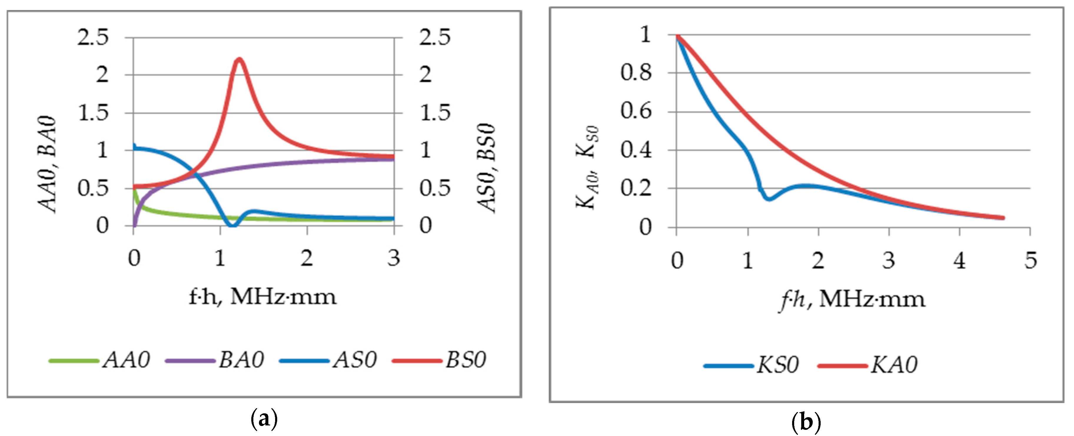
Since the main type of AE waves are Lamb waves, it is necessary to consider that the presence of dispersion significantly affects the behavior of the attenuation coefficient for these modes. The attenuation coefficient of the Lamb waves is a linear combination of the attenuation coefficients of the longitudinal wave α and transverse wave β, respectively [18]:
where AS0, BS0, AA0 and BA0 are coefficients that are determined by the type of Lamb wave. The graphs in Figure 1a show that AS0, BS0, AA0 and BA0 significantly depend on the f·h parameter.
The energy loss can be described by the transmission coefficients KA0, KS0, which correspond to the exponential dependence on length and frequency
where γA0 and γS0 are the attenuation coefficients for the Lamb wave’s zero-modes, and is the propagation distance. The dependences of the transmission coefficients on parameter f·h are shown in Figure 1b.
2.3. AE Sensor Modeling
For the modeling results to be of practical importance, it is necessary to consider the features of AE wave detection—i.e., the transfer function of the AE sensor. During propagation, Lamb waves because displacements oriented in both the transverse and longitudinal directions. The AE sensor, as a rule, is oriented in such a way that it detects only the normal components of displacement. The proportion of the longitudinal and transverse components in the displacement vector has a complicated frequency dependence. The dependences of the amplitudes of the longitudinal and transverse components of the displacements on frequency are given in [18]. Based on these dependences, the transverse fractions vs. frequency for the modes A0(δA0) and S0(δS0) were calculated.
As can be seen in Figure 2a, the transverse component for the mode A0 prevails in the region of the small values of f·h. The fraction of transverse component δS0 for the mode S0 in the region of small f·h values is close to zero. Then, it gradually increases and approaches unity in the region of maximum dispersion of f·h ~ 1.25 MHz·mm.
A resonant sensor GT200 (Global Test LLC) with a resonant frequency of 180 kHz, and 16 mm in diameter and 15 mm in high is considered to be an example of an AE sensor. This sensor is characterized by relatively high sensitivity and is widely used for industrial control. The frequency response of the sensor is shown in Figure 2b.
2.4. Simulation Method Description
The modelling procedure is based on the Lamb waves modal analysis results. The basic AE signal waveform uA0,S0(z,t) is calculated analytically as a reaction of the waveguide on a point excitation, which is set as a δ-function. The A0 and S0 modes are modeled separately. The transmission coefficient and sensor transfer functions are set in the frequency domain and could be interpreted as a linear frequency filter with a transfer function HA0,S0(f) equal to the production of three functions—the transfer coefficient KA0,S0(f), the frequency dependent part of the normal component of displacement vector δA0,S0, and the sensor frequency response S(f)
The frequency-sampling method has been applied to transform the transfer function HA0,S0 into a finite impulse response, which could be represented in a discrete form using Equation (15):
where Δf is the sampling frequency interval, and N is the number of frequency samples [19].
Ultimately, the modeled signal is obtained as a result of the convolution of uA0,S0 and hA0,S0. The scheme of the simulation algorithm is shown in Figure 3.
Modeling was carried out for wall thicknesses from 3 to 40 mm, with propagation distances from 0.5 to 50 m. The acoustic parameters of carbon steel were used: ρ = 7800 kg/m3, cL = 5900 m/s, cT = 3100 m/s. Signals arriving in the form of an S0 or A0 wave were modeled separately. An equal ratio of the energies of the S0 and A0 modes was set. The sampling frequency of the simulated signal was equal to 1000 kHz, and its duration ranged from 4096 to 16,384 μs. A single impulse with a 1 μs duration was used as the emitted signal.
2.5. Experiment Description
Verification of the simulation results was carried out by comparing the modeled data with AE impulses obtained experimentally. The experiments were carried out in the factory and field conditions at industrial facilities (trunk and technological pipelines).
The experiment was carried out as follows. An AE sensor was installed on the pipeline surface at a certain distance from the emission point. AE waves were simulated using the Hsu–Nielsen source [20], under the assumption that the impulse from a pencil-lead break in some approximation can be considered as a δ-function. An example of the trunk pipeline used for experimental investigation is shown in Figure 4a, and the scheme of the experiment is shown in Figure 4b.
This approach to set up the experiment allows a more complete and reliable comparison of the simulation results and the experimental results. It also allows us to use the signals obtained as a result of modeling as reference signals for the AE data processing algorithms intended for industrial applications.
To verify the model, the data of two experiments were selected, corresponding to the minimum and maximum values of the pipe wall thickness. The first object is the trunk gas pipeline with a diameter of 1020 mm and a wall thickness of 17 mm made of structure carbon steel 17GS. The second is a technological pipeline with a diameter of 500 mm and a wall thickness of 9 mm, which was also made of structure carbon steel 20. Measurements were performed using an A-Line-32D PCI system produced by “INTERUNIS-IT” corporation with GT200 sensors [21] and a PAEF-014 preamplifier with a bandwidth of 30–500 kHz and a gain of 26 dB.
3. Results
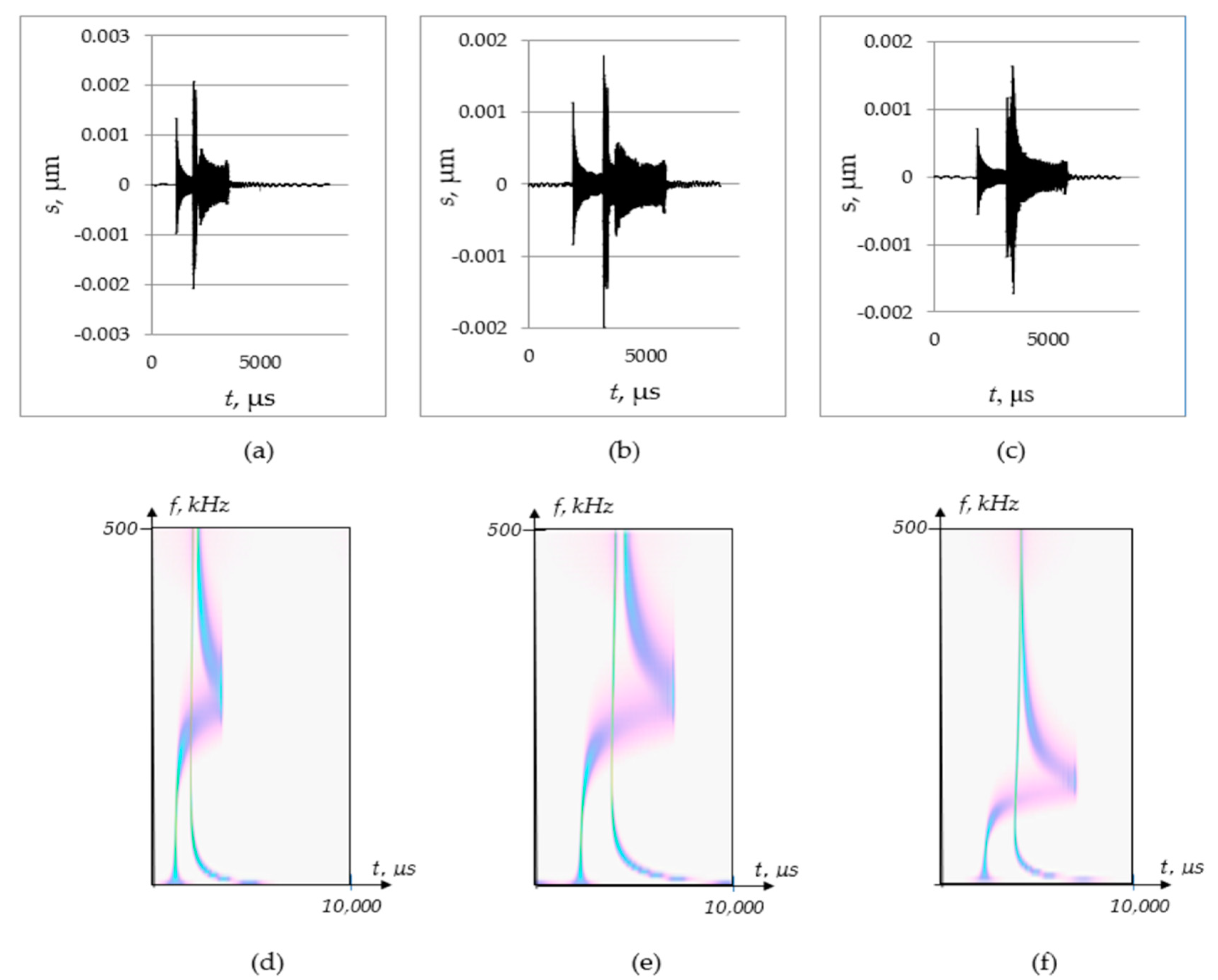
This section contains the AE signals modeling results and verification of the simulation results and experimental data. Figure 5 shows the results of the modal analysis without the influence of signal absorption. Signals and their spectrograms simulating the propagation of Lamb wave zero modes for objects with different thicknesses and waveguide lengths are represented.
Figure 5a,b shows that, with an increase in the path length, the signal duration increases due to a larger difference in the arrival times of the A0 and S0 modes frequency components. It should be noted that dispersive propagation also leads to a decrease in the peak of the AE signal due to the delocalization of various components of the signal. Figure 5b,c shows that a change in thickness affects the phase-frequency structure of the signal, while dispersion curves shift with increasing thickness toward lower frequencies.
Figure 6a–d shows the model signals calculated considering all the influencing factors included in the modeling algorithm. The represented signals correspond to one distance between the AE source and the sensor, but different wall thickness values. Comparing the waveforms of the A0 and S0 modes, we can conclude that the waveform of the S0 mode is more dependent on the waveguide thickness than the waveform of the A0 mode. Frequency-dependent parameters, such as the transmission coefficient and the normal component of the extrema coordinates of the S0 mode, have an extremum depending on the f·h value. The complex correlation of the coordinates of the extrema for dependences KS0(f) and δS0(f), considered together with the resonant sensor transfer function, leads to the strong influence of waveguide thickness on the S0-mode waveform, which is characterized by a lower transmission coefficient and a lower dispersion for small thicknesses of about 5–9 mm, and a larger transmission coefficient and greater dispersion for wall with thicknesses greater than 15 mm.
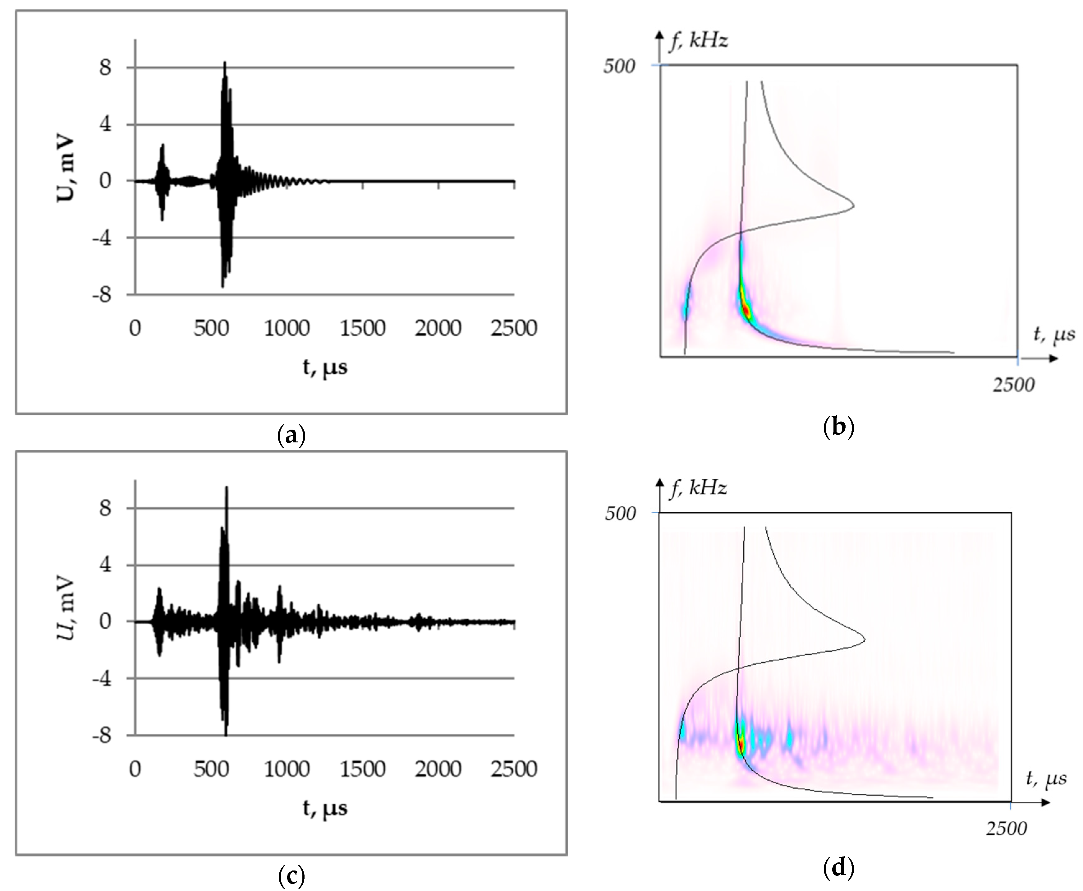
To verify the model while considering the attenuation coefficients of the Lamb waves, we compared the simulation results with the experimental results described in Section 2.5. The simulated and measured signals corresponding to the same waveguide parameters are presented in Figure 7 and Figure 8.
The signals corresponding to the waveguide length equal to 6 m and thickness equal to 9 mm are represented in Figure 7a,c, and wavelet transforms are represented in Figure 7b,d. The experimental waveguide was the technological pipeline with a diameter of 500 mm. Comparing the simulated and experimental signals, we can conclude a high degree of correspondence; the ratio between the A0 and S0 mode amplitudes is equal to 3.7 for the simulated signal and 4.0 for the signals obtained experimentally. The time intervals between the A0 and S0 peaks are 421 μs and 429 μs for the simulated and measured data, respectively.
The superposition of group velocities in the wavelet transforms (Figure 7b,d) confirms the correctness of the modeling procedure due to the similarity of the relative intensities of the two main modes. On the time-frequency plane (Figure 7d), one can see the fragments associated with the multipath wave propagation that were not taken into account when calculating the model signal. However, these signal components are characterized by relatively low energy and do not greatly affect the waveform. It should also be noted that the experimentally obtained signal has a lower frequency spectrum. This fact could be explained by the difference in the frequency characteristics of the simulated sensor and the sensor used in the experiment or by the influence of the couplant properties that were not simulated. The correlation coefficient between the simulated and experimental signals is equal to 0.58.
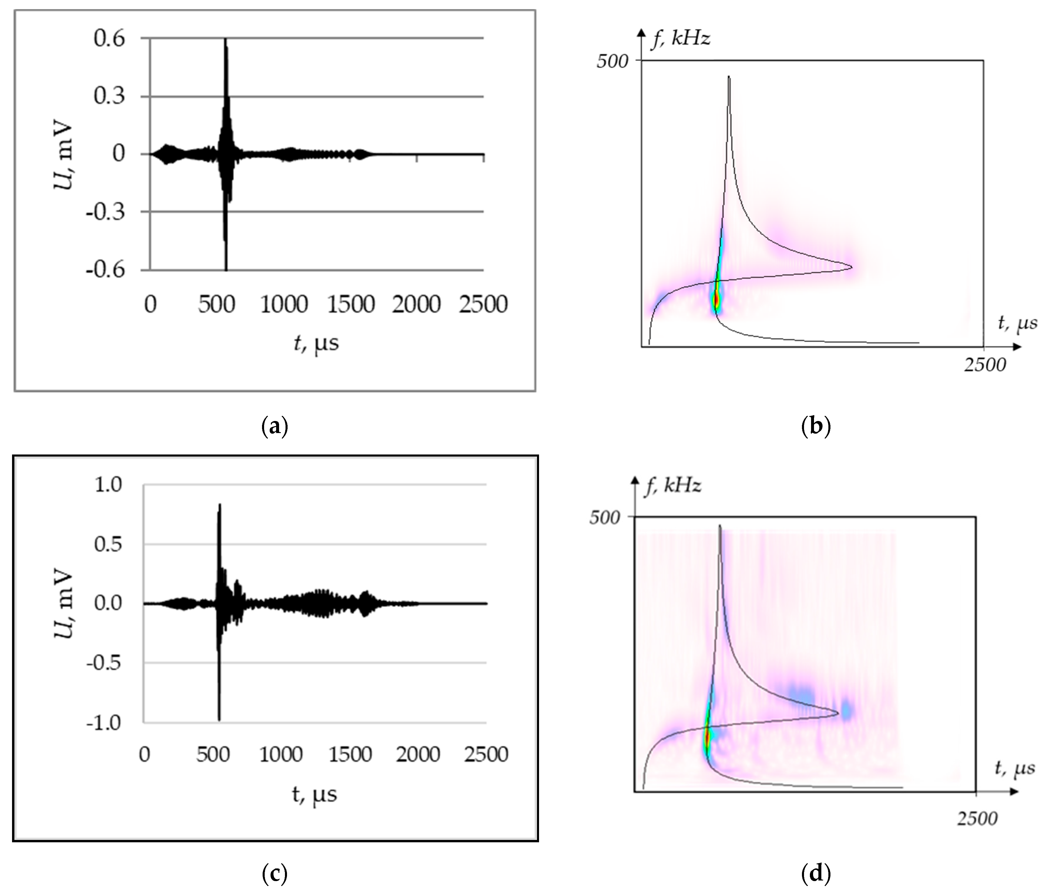
The signals corresponding to the waveguide length that equals 4 m with a thickness equaling 17 mm are represented in Figure 8a,c, and the wavelet spectrograms are represented in Figure 8b,d. The experimental object was the trunk pipeline with a diameter of 1020 mm. The experimental and simulated signals are visually similar, which could be confirmed by a correlation coefficient of 0.72. The wavelet spectrogram corresponding to the measured signal also has additional modes propagating along numerous possible paths between the AE source and the sensor. The superimposition of the group velocities on the wavelet transform shows that the A0 and S0 modes are localized identically on the time-frequency plane for the simulated and experimental data.
4. Discussion
The results obtained in this paper allow us to conclude that the modal analysis of the normal waves propagation, supplemented by an analytical calculation of Lamb wave attenuation, is an effective analytical method for calculating the propagation of AE signals along a waveguide. Using this method, signals that possess all the characteristic features of real signals in the shapes of their envelopes, their frequency spectrum and their spectrograms were obtained. To obtain a realistic form of model signals, it is necessary to consider all the components of the transmission coefficient: phase changes caused by the dispersion propagation of Lamb waves, the attenuation coefficient, and the characteristics of the AE sensor.
The S0 wave is more susceptible to dispersive propagation in the considered frequency range from 30 to 500 kHz; as a result, the signal duration corresponding to the S0 mode is longer, and the peak amplitude, as a rule, is smaller than that of the A0 mode, even in the case of equal energy radiated in the form of these modes. The maximum mode transmission coefficient, A0, corresponds to the low-frequency region. The attenuation parameters of the A0 mode are determined mainly by the distance between the source and receiver of the AE waves and, to a small extent, depend on the thickness. The parameters of the passage of the S0 mode substantially depend on the thickness and, to a lesser extent, on the distance. The conditions for receiving the transverse component of the S0 mode oscillations are unfavorable due to the mismatch of the frequency ranges of the minimum attenuation coefficient and the maximum fraction of the transverse component of the S0 mode.
Verification of the model was carried out by comparing the modeled signals with the signals obtained experimentally using a Hsu-Nielsen source. During this comparison, the waveform of the simulated and experimental signals, established to show a high degree of similarity between them, even though the experiment to simulate AE impulses was carried out under field conditions at industrial pipelines. The influence of factors such as the presence of welded joints, shutoff valves, as well as the presence of a light degree corrosion damage with a depth of up to 10% of the pipe wall’s thickness did not significantly affect the similarity of the waveform between the real and modelled signals. The correlation coefficient, which can be interpreted as a numerical estimation of the waveform similarity, is about 0.6 due to the influence of multipath guided wave propagation, which was not taken into account due to differences between the transfer function of the reference sensor and the AE sensor that was used during the experiment.
When applying the simulation results as reference signals, it should be considered that the signal from the defect does not fully correspond to the signal of the Hsu–Nielsen source. Hamstad [4] established that the Hsu-Nielsen source corresponds to the monopole model, while stress-generated AE sources are almost universally composed of dipoles. In addition, it is necessary to consider that the simulation results presented in this paper correspond to a case when the source is located out-of-plane, while the depth of the stress-generated AE source is uncertain. Hamstad [4] and Giurgiutiu [15] determined that the main difference between the in-plane and out-of-plane sources consists of the relationship between the A0 and S0 mode amplitudes. Since the relationships between the mode amplitudes are established in the papers [4,15], this uncertainty could be considered due to the addition of a weighted coefficient for each mode, which is simulated separately in accordance with the scheme in Figure 3.
Based on the result of the model verification, we can conclude that the analytically modeled signals could be used as reference signals for the AE signal filtration and as training sets for AE data processing algorithm verification. The obtained results seem more realistic than a formal mathematical model and are simpler and more available to a wide range of researchers than the FEM model. The modeled signal waveform includes the characteristic features that are important from the perspective of signal processing.
5. Conclusions
In this work, the algorithm for AE impulse waveform simulation was developed. This algorithm is based on the modal analysis of Lamb wave propagation, which was supplemented with an analytical calculation of scattering and the frequency response of the AE sensor. The theoretical basis used for this simulation algorithm is not novel. However, the integration of various theoretical methods allowed us to obtain the algorithm for AE impulse simulation, which is simple and useful from the perspective of practical significance. The authors hope that this potential algorithm and the presented results (along with their use) will be useful for researchers and engineers specializing in AE data processing methods.
Author Contributions
Conceptualization, S.E.; methodology, V.B. (Vera Barat) and D.T.; validation, V.B. (Vera Barat) and D.T.; formal analysis, D.T.; investigation, V.B. (Vera Barat), D.T. and V.B. (Vladimir Bardakov); resources, V.B. (Vera Barat), D.T. and V.B. (Vladimir Bardakov); data curation, V.B. (Vera Barat) and D.T.; writing—original draft preparation, V.B. (Vera Barat), D.T. and V.B. (Vladimir Bardakov); writing—review and editing, V.B. (Vladimir Bardakov); visualization, V.B. (Vladimir Bardakov) and V.B. (Vera Barat); supervision, V.B. (Vera Barat) and S.E.; project administration, S.E. All authors have read and agreed to the published version of the manuscript.
Funding
The work was carried out in the implementation of State Order Project of Ministry of Education and Science of Russian Federation in the field of scientific activity № 11.9879.2017/8.9.
Conflicts of Interest
The authors declare no conflict of interest.
References
- Lowe, M.J.S. Matrix techniques for modelling ultrasonic waves in multi-layered media. IEEE Trans. Ultrason. Ferroelectr. Freq. Control 1995, 47, 525–542. [Google Scholar] [CrossRef]
- Krushynska, A.A.; Meleshko, V.V. Normal waves in elastic bars of rectangular cross section. J. Acoust. Soc. Am. 2011, 129, 1324–1335. [Google Scholar] [CrossRef] [PubMed]
- Kuo, C.W.; Suh, C.S. On the dispersion and attenuation of guided waves in tubular section with multi-layered viscoelastic coating—Part I: Axial wave propagation. Int. J. Appl. Mech. 2017, 9, 1750001. [Google Scholar] [CrossRef]
- Hamstad, M.A. Acoustic emission signals generated by monopole (pencil-lead break) versus dipole sources: Finite element modeling and experiments. J. Acoust. Emiss. 2007, 25, 92–106. [Google Scholar]
- Hamstad, M.A. Frequencies and Amplitudes of AE Signals in a Plate as a Function of Source Rise Time. In Proceedings of the 29th Conference of the European Working Group on Acoustic Emission (EWGAE), Vienna, Austria, 8–10 September 2010; p. 8. [Google Scholar]
- Sause, M.G.R. Modelling of Crack Growth Based Acoustic Emission Release in Aluminum Alloys. In Proceedings of the 31st Conference of the European Working Group on Acoustic Emission (EWGAE), Dresden, Germany, 3–5 September 2014; p. 8. [Google Scholar]
- Alexandre, J.M.; Antunes, M.S.; Regina, C.P.; Leal-Toledo, D.S.; Otton Teixeira da Silveira Filho, D.S.; Elson Magalhaes Toledo, D.S. Finite Difference Method for Solving Acoustic Wave Equation Using Locally Adjustable Time-steps. Procedia Comput. Sci. 2014, 29, 627–636. [Google Scholar]
- Loveday, P.W. Semi-analytical finite element analysis of elastic waveguides subjected to axial loads. Ultrasonics 2009, 49, 298–300. [Google Scholar] [CrossRef] [PubMed]
- Cho, Y.; Rose, J.L. A boundary element solution for mode conversion study of the edge reflection of Lamb waves. J. Acoust. Soc. Am. 1996, 99, 2097–2109. [Google Scholar] [CrossRef]
- Lowe, M.J.S.; Cawley, P. The applicability of plate wave techniques for the inspection of adhesive and diffusion bonded joints. J. Nondestruct. Eval. 1994, 13, 185–200. [Google Scholar] [CrossRef]
- Fornberg, B. The pseudospectral method; accurate representation of interfaces in elastic wave calculations. Geophysics 1998, 53, 625–637. [Google Scholar] [CrossRef]
- Migot, A.; Giuriutiu, V.; Bhuiyan, M.Y. Numerical and experimental investigation of damage severity estimation using Lamb wave–based imaging methods. J. Intell. Mater. Syst. Struct. 2018, 30, 1–8. [Google Scholar] [CrossRef]
- Prakash, R.; Li, L.; Haider, M.F.; Giurgiutiu, V. Hybrid SAFE-GMM approach for predictive modeling of guided wave propagation in layered media. Eng. Struct. 2019, 193, 194–206. [Google Scholar]
- Mei, H.; Haider, M.F.; Joseph, R.; Migot, A.; Giurgiutiu, V. Recent advances in piezoelectric wafer active sensors for structural health monitoring applications. Sensors 2019, 19, 383. [Google Scholar] [CrossRef] [Green Version]
- Haider, M.F.; Bhuiyan, M.Y.; Poddar, B.; Lin, B.; Giurgiutiu, V. Analytical and experimental investigation of the interaction of Lamb waves in a stiffened aluminum plate with a horizontal crack at the root of the stiffener. J. Sound Vib. 2018, 431, 212–225. [Google Scholar] [CrossRef]
- Li, J.; Rose, J.L. Excitation and propagation of non-axisymmetric guided waves in a hollow cylinder. J. Acoust. Soc. Am. 2001, 109, 457–464. [Google Scholar] [CrossRef] [PubMed]
- Seco, F.; Jiménez, A.R. Modelling the generation and propagation of ultrasonic signals in cylindrical waveguides. In Ultrasonic Waves; InTech: London, UK, 2012; pp. 1–28. [Google Scholar] [CrossRef] [Green Version]
- Viktorov, I. Rayleigh and Lamb Waves. In Physical Theory and Applications, 1st ed.; Springer: Berlin/Heidelberg, Germany, 1967; p. 154. [Google Scholar]
- Ifeachor, E.; Jervis, B. Digital Signal Processing: A Practical Approach, 2nd ed.; Prentice Hall: Upper Saddle River, NJ, USA, 2001; p. 960. [Google Scholar]
- Pollock, A. Acoustic Emission amplitude distribution. In International Advances in Nondestructive Testing; Gordon and Breach: New York, NY, USA, 1981; Volume 7, pp. 215–240. [Google Scholar]
- Official Website of «GlobalTest» Company. Available online: http://globaltest.ru/ru/katalog/datchiki/reobrazovateli-akusticheskoj-ehmissii/ (accessed on 10 October 2019).
Figure 1.
Dependencies of (a) AS0, BS0, AA0 and BA0 vs. f·h; (b) the transmission coefficients KA0 and KS0 vs. f·h.
Figure 1.
Dependencies of (a) AS0, BS0, AA0 and BA0 vs. f·h; (b) the transmission coefficients KA0 and KS0 vs. f·h.

Figure 2.
(a) Dependence of the transmittance on frequency for different thicknesses (from 5 to 30 mm) of the object and the distance l = 6 m: red for mode A0 and blue for mode S0; (b) The frequency response of the sensor.
Figure 2.
(a) Dependence of the transmittance on frequency for different thicknesses (from 5 to 30 mm) of the object and the distance l = 6 m: red for mode A0 and blue for mode S0; (b) The frequency response of the sensor.

Figure 3.
The scheme of the simulation algorithm.

Figure 4.
(a) An example of the trunk pipeline used for the experiment; (b) the simulation experiment scheme.
Figure 4.
(a) An example of the trunk pipeline used for the experiment; (b) the simulation experiment scheme.

Figure 5.
Model signals and wavelet spectrograms of the model signals at different waveguide lengths and wall thicknesses: (a,d) a thickness of 9 mm and a distance of 5 m; (b,e) a thickness of 9 mm and a distance of 10 m; (c,f) a thickness of 17 mm and a distance of 10 m.
Figure 5.
Model signals and wavelet spectrograms of the model signals at different waveguide lengths and wall thicknesses: (a,d) a thickness of 9 mm and a distance of 5 m; (b,e) a thickness of 9 mm and a distance of 10 m; (c,f) a thickness of 17 mm and a distance of 10 m.

Figure 6.
Model signals calculated for a waveguide length of 5 m and various thicknesses (the blue graph is mode S0, and the red graph is mode A0): (a) h = 5 mm; (b) h = 9 mm; (c) h = 17 mm; (d) h = 30 mm.
Figure 6.
Model signals calculated for a waveguide length of 5 m and various thicknesses (the blue graph is mode S0, and the red graph is mode A0): (a) h = 5 mm; (b) h = 9 mm; (c) h = 17 mm; (d) h = 30 mm.

Figure 7.
Comparison of the modelled and experimental AE signals for a waveguide length of 6 m and a thickness of 9 mm: (a) the simulated signal, (b) the wavelet transform for the simulated signal and a superimposition of group velocities, (c) the measured signal, and (d) the wavelet transform for the measured signal and the superimposition of group velocities.

Figure 8.
Comparison of model and experimental AE signals for the waveguide length of 4 m and a thickness of 17 mm: (a) simulated signal, (b) the wavelet transform for the simulated signal and the superimposition of group velocities, (c) the measured signal, and (d) the wavelet transform for the measured signal and the superimposition of group velocities.

© 2019 by the authors. Licensee MDPI, Basel, Switzerland. This article is an open access article distributed under the terms and conditions of the Creative Commons Attribution (CC BY) license (http://creativecommons.org/licenses/by/4.0/).
Share and Cite
MDPI and ACS Style
Barat, V.; Terentyev, D.; Bardakov, V.; Elizarov, S. Analytical Modeling of Acoustic Emission Signals in Thin-Walled Objects. Appl. Sci. 2020, 10, 279. https://doi.org/10.3390/app10010279
AMA Style
Barat V, Terentyev D, Bardakov V, Elizarov S. Analytical Modeling of Acoustic Emission Signals in Thin-Walled Objects. Applied Sciences. 2020; 10(1):279. https://doi.org/10.3390/app10010279
Chicago/Turabian StyleBarat, Vera, Denis Terentyev, Vladimir Bardakov, and Sergey Elizarov. 2020. "Analytical Modeling of Acoustic Emission Signals in Thin-Walled Objects" Applied Sciences 10, no. 1: 279. https://doi.org/10.3390/app10010279
Note that from the first issue of 2016, this journal uses article numbers instead of page numbers. See further details here.