A Random Factorial Design of Experiments Study on the Influence of Key Factors and Their Interactions on the Measurement Uncertainty: A Case Study Using the ZEISS CenterMax

Abstract

This paper addresses the uncertainty analysis in the case of a coordinate measuring machine. The main goal was analyzing, quantifying, and drawing conclusions on the influence of key factors and their interactions on the measurements’ uncertainty of the variable’s parallelism, angularity, roundness, diameter, and distance. In order to achieve this goal, a Random Factorial Design of Experiments was designed and implemented. It focused on the factors Stylus diameter, Step width, and Speed using three random levels each. For the solution of the experiment, an analysis of variance was used. The study was carried out on the coordinate measuring machine (CMM) ZEISS CenterMax. It was concluded that the interaction effects among Stylus diameter, Step width, and Speed were active at a confidence level of 95%. Besides, it was possible to estimate random factors‘ variance and their contribution to the total variation. Among the main effects, the Stylus diameter showed to be the one with the biggest influence. The paper also quantifies the influence in the measurement uncertainty, where the highest value of standard uncertainty belonged to the Stylus diameter in the evaluation of the variable’s angularity and diameter. Besides, the Speed factor was proved to have the biggest influence on the roundness’ measurement and evaluation.

1. Introduction

In manufacturing, parts and pieces are often affected by form and size errors that have to be assessed against geometrical and dimensional tolerances in order to prove their conformance with given specifications [1]. In this regard, when referring to the measurement result of a physical quantity, it becomes necessary to offer valuable measurable proof of the quality of the result in a way that people using it afterward can assess its reliability. Without such quantifiable value, it is then impossible to compare measurement results, either among themselves or to established values appearing in a specification or standard [2]. Generally speaking, this guide considers within its definitions that measurement uncertainty is a parameter that characterizes the dispersion of the values that could reasonably be attributed to the measurand. It also states that some of its components may be evaluated from the statistical distribution of the results of a series of measurements and can be characterized by experimental standard deviations. Similarly, as cited in [3], according to the ISO/IEC 17025, estimating measurement uncertainty is required for all laboratories accredited to this standard, which adds even more relevance to this whole issue. This is something that has remained key in other versions of the standard including the last one from 2017.

In today’s industrial production, the coordinate measuring machine (CMM) is one of the cornerstones of inspection in most enterprises. Without a CMM, it is difficult to imagine the evaluation of measuring parameters related to simple dimension measurement based on drawings, and this is not to mention complex endeavors, such as evaluation of form, location, and position deviations or the offset of certain points from a 3D model [4]. They are complex measuring instruments able to reconstruct the sampled surface for reverse engineering and verify dimensions and features.

Essentially, CMMs are sophisticated units that are usually intended to be operated in the controlled environment of a metrology laboratory. The clear majority of the methods and approaches for the measurement of uncertainty in CMM can be classified as mathematical, comparative, and performance test ones. The first group of these, also referred to as mathematical modeling methods, encompasses the same calibration of the CMM geometric errors, which is the base for the posterior creation of a theoretical model that allows predicting the uncertainty for all measurements executed according to the model’s assumptions [5]. On the other hand, comparison methods usually involve the measurement of an “identical” calibrated part, often referred to as artifact. These methods are flexible to an extent and, thus, the effect of form errors would have to be quite often included in the overall uncertainty measurement. As for the performance test methods, these usually designate artifacts and define a criterion for obtaining the measurement errors, where, usually, a two-point length measurement uncertainty is defined as a performance parameter [6]. These performance test approaches are ones that more precisely relate to the content of this paper and, thus, ones to be used and further described in the following sections.

When using a CMM to measure a technical object, many factors affect measurement uncertainty [7]. In this regard, numerous studies in the field of measurement uncertainty in CMM have been conducted, mainly focused on accuracy improvement by developing hardware, software, and operating strategies [8,9]. On the other hand, most CMM tasks do not have a rigorous uncertainty budget. In fact, most of the uncertainty in these cases is simply a guess from an experienced operator [10]. In an attempt to target this issue and others related, the ZEISS Metrology Academy developed the book “Cookbook” [11], which provides the most common measurement strategies and allows the CMM operators to design the measurement path and perform and evaluate these. The book contains a wide range of strategies and tables with “proved” values for comparable measurements, based mainly on the company’s experience, which introduces an empirical component that, at times, fails and misses to be backed up by theories and methods in the state of the art and practice, i.e., mainly proper statistical validation and methods. Besides, even when it is a good reference and offers valuable resources to the person carrying out the measurements, the book is mainly intended for basic operation, general tasks, and short-term courses where, again, there is usually no time to statistically analyze or back up most of the results.

Based on the literature review consulted within this contribution, this lack of theoretical knowledge (proper statistical validation and methods) generally applies to the whole operation with CMM. In the end, it can be all easily reflected in how the staff frequently is left to decide on certain factors at the time of conducting a given measurement.

Regardless of the type of system, in order to really understand cause-and-effect relationships in one of these, one must often deliberately change the input variables to the system and observe the changes in the system output that these changes to the inputs produce. However, even in the selected reference literature analyzed for this paper, there is a lack of statistical demonstration covering the selection of the suggested values and demonstrating how randomly varying one of the levels of a given factor or their interactions is then reflected in the uncertainty associated with the measurements.

In this regard, the statistical design of experiments (DOE) is precisely, among a few others, one of the most effective ways to test and analyze these phenomena, given that it provides the necessary technique and strategy to efficiently carry the processes to better operating conditions. In its core, the DOE consists of inducing the variability of measurement errors and, in this regard, it is precisely the statistical analysis of variance (ANOVA) that is usually recommended and used for processing and achieving a better interpretation of the results.

Authors like [12] provided a review of the different works carried out in this field, where the authors pointed out that of the number of studies reported about evaluating measurement uncertainty, few had applied the factorial design to study the uncertainty measurement, the statistical significance of the factors that affect the process of measurement, and the interaction between them. For example, the studies of [13,14] were based on the mean absolute percent error. On the other hand, [15] used simulation techniques to estimate measurement uncertainty when measuring small circular features and compared the results with experimental studies. These authors presented a simple experimental design that, in the opinion of the authors of this contribution, lacks the presence of multiple factors, therefore failing to properly analyze and conclude on the impact of their interactions.

The research conducted by [7] applies the DOE approach to investigate the impact of the factors and their interactions on the uncertainty while following the fundamental rules defined in the ISO Guide to the Expression of Uncertainty in Measurement (GUM). Additionally, in the study of [16], these authors used a factorial design to implement a performance test and investigate CMM errors associated with the length and orientation in the work volume. Both studies consider only two levels of analysis by factor and the value of the uncertainty associated with the variation of the levels is not quantified.

The previous studies have contributed to the analysis of one or quite a few factors, though none of them have however systematically examined the Step width, Stylus diameter, and measuring Speed when executing the measurement. One parameter or another had been neglected, whether it was the factors themselves or the factor interactions, which is another motivation behind this research. Furthermore, none of these studies have included an analysis of many variables.

Based on these analyses, there are evident gaps in the state of the art and practice. Unlike previous studies, this paper presents an experimental design of three random factors and three levels each, i.e., (33), for the purposes of assessing the uncertainty of the CMM measurement of five variables: parallelism, angularity, roundness, diameter, and distance. In order to complement this, an ANOVA was implemented to improve the evaluation of the results, estimate the interaction between factors, and determine and quantify the contribution of variables to the measurement uncertainty. Measurements of the study case analyzed in this paper were performed using a ZEISS CenterMax CMM at the Faculty of Materials Science and Technology in Trnava, Slovakia. The rest of this contribution is divided as follows: Section 2, Materials and Methods; Section 3, Results and Discussion; Section 4, Conclusions; and the final section containing the References.

2. Materials and Methods

In the state of the art and practice, one can usually find many techniques and approaches to design an experiment. The author in [17] introduces certain DOE techniques named factorial design, where experimental variables are investigated in all possible combinations of their factors or levels and the results are analyzed by ANOVA. These group of techniques caught the attention of the scientific community given their many applications to deeply analyze and even help quantifying the impact of such factors and their interactions on a given dependent variable or output response of the system, through the strategy of experimentation, i.e., the measurement accuracy and/or precision defined by the uncertainty quantification in the context of this paper.

On the other hand, the factorial designs involve that, in each complete trial or replicate of the experiment, all possible combinations of the levels of the factors are investigated, and that is precisely what makes it most efficient for this type of analyses and the specific case study targeted within this paper.

Before selecting the DOE type and conducting a performance test, it is first always necessary to consider the time available for the realization of all experimental runs. This time keeps a direct relation to the number of experimental variables, the number of their levels, and the amount of data required. In a factorial design, the total number of runs n is determined using the expression n = l^k, where l is the number of levels of each factors and k is the number of experimental variables investigated (factors); in other words, it is usually and simply the mere calculation of the number of combinations. For example, in the particular case of having three variables with three levels each, the total number of runs is 33 and is equal to 27 [12]. In turn, this value must be multiplied by the number of replicates of the experiment. Replicates are multiple experimental runs with the same factor settings (levels), subject to the same sources of variability, independently of each other.

In some experimental situations, the factor levels are chosen at random from a larger population of possible levels, and the experimenter wishes to draw conclusions about the entire population of levels, not just those that were used in the experimental design. The application of a random-effects model entails the need to consider the uncertainty associated with the random choice of test levels. In other words, it means it no longer makes sense for factor A to worry about the effect a_i of level i. In these cases, what becomes important is to estimate the variance the random factor contributes to and/or influences with the total variation, and to test if this is significant.

If the experiment is replicated n times, it may be useful to represent the observations by a linear statistical model, as is shown in Equation (1) for the case of a 33-factorial design.

$$\begin{array}{cc}\begin{array}{c}{y}_{ijkl}=\mu +\tau {}_i+{\beta }_j+{\gamma }_k+{\left(\tau \beta \right)}_{ij}+\\ {\left(\tau \gamma \right)}_{ik}+{\left(\beta \gamma \right)}_{jk}+{\left(\tau \beta \gamma \right)}_{ijk}{+}_{ijkl}\end{array}& \{\begin{array}{c}i=1,\dots a\\ j=1,\dots b\\ \begin{array}{c}k=1,\dots c\\ l=1,\dots n\end{array}\end{array}\end{array}$$

(1)

In this model, $y_{ijkl}$ represents the response variable, for example, the measurement error; ${\tau }_i$ is i-th level effect of the A factor; ${\beta }_j$ is the j-th level effect of the B factor; ${\gamma }_k$ is the k-th level effect of the C factor; and ${\left(\tau \beta \right)}_{ij,}$ ${\left(\tau \gamma \right)}_{ik},{\left(\beta \gamma \right)}_{jk},{\left(\tau \beta \gamma \right)}_{ijk}$ I is the effect of the interaction between factors. The letters a, b, and c correspond to the number of levels for each factor, respectively, and r is the number of replicates, and where the model parameters are independent of the residual error ${\epsilon }_{ijkl}$, normally distributed with mean zero and value variances NID (0,${\sigma }_T^2$). The variance of any observation is given by Equation (2).

$${\sigma }_y^2={\sigma }_{\tau }^2+{\sigma }_{\beta }^2+{\sigma }_{\gamma }^2+{\sigma }_{\tau \beta }^2+{\sigma }_{\tau \gamma }^2+{\sigma }_{\beta \gamma }^2+{\sigma }_{\tau \beta \gamma }^2+{\sigma }^2$$

(2)

The ANOVA for this case can be seen in

Table 1. Analysis of variance. 33-factorial design.

Source of Variation	Sum of Squares	Degrees of Freedom	Mean Squares	Calculated F
A	SSA	a − 1	$MSA=\frac{SSA}{DFA}$	$F=\frac{MSA+MSABC}{MSAB+MSAC}$
B	SSB	b − 1	$MSB=\frac{SSB}{DFB}$	$F=\frac{MSB+MSABC}{MSAB+MSBC}$
C	SSC	c − 1	$MSC=\frac{SSC}{DFC}$	$F=\frac{MSC+MSABC}{MSAC+MSBC}$
AB	SSAB	(a − 1)(b − 1)	$MSAB=\frac{SSAB}{DFAB}$	$F=\frac{MSAB}{MSABC}$
AC	SSAC	(a − 1)(c − 1)	$MSAC=\frac{SSAC}{DFAC}$	$F=\frac{MSAC}{MSABC}$
BC	SSBC	(b − 1)(c − 1)	$MSBC=\frac{SSBC}{DFBC}$	$F=\frac{MSBC}{MSABC}$
ABC	SSABC	(a − 1)(b − 1)(c − 1)	$MSABC=\frac{SSABC}{DFABC}$	$F=\frac{MSABC}{MSR}$
Residual	SSR	abc(n − 1)	$MSR=\frac{SSR}{DFR}$
Total	SST	abcn − 1

. The mean square (MS) could be assumed as an estimate of the variance and determined using the sum of squares (SS), then divided by the respective degrees of freedom (DF). It is necessary to clarify that, as MS values were calculated using all measurement errors, all components of variance require the compensation of the residual variation present in the determined MS. It may be shown that expected mean squares (EMS) are a function of variables, interaction, and residual components of variance, as given in Equations (3)–(10) [17].

$$E\left(MSA\right)={\sigma }^2+cn{\sigma }_{\tau \beta }^2+bn{\sigma }_{\tau \gamma }^2+n{\sigma }_{\tau \beta \gamma }^2+bcn{\sigma }_{\tau }^2$$

(3)

$$E\left(MSB\right)={\sigma }^2+cn{\sigma }_{\tau \beta }^2+an{\sigma }_{\beta \gamma }^2+n{\sigma }_{\tau \beta \gamma }^2+acn{\sigma }_{\beta }^2$$

(4)

$$E\left(MSC\right)={\sigma }^2+bn{\sigma }_{\tau \gamma }^2+an{\sigma }_{\beta \gamma }^2+n{\sigma }_{\tau \beta \gamma }^2+abn{\sigma }_{\gamma }^2$$

(5)

$$E\left(MSAB\right)={\sigma }^2+n{\sigma }_{\tau \beta \gamma }^2+cn{\sigma }_{\tau \beta }^2$$

(6)

$$E\left(MSAC\right)={\sigma }^2+n{\sigma }_{\tau \beta \gamma }^2+bn{\sigma }_{\tau \gamma }^2$$

(7)

$$E\left(MSBC\right)={\sigma }^2+n{\sigma }_{\tau \beta \gamma }^2+an{\sigma }_{\beta \gamma }^2$$

(8)

$$E\left(MSABC\right)={\sigma }^2+n{\sigma }_{\tau \beta \gamma }^2$$

(9)

$$E\left(MSE\right)={\sigma }^2$$

(10)

The F tests are performed to control the statistical significance of the variable and interaction effects at a given probability. However, when working with random factorial designs of the type 3³, a procedure attributed to [18] is the one to be used. Satterthwaite’s method uses linear combinations of mean squares, as it appears below in Equations (11)–(12).

$$M{S}^{\prime }=M{S}_r+\cdots +M{S}_s$$

(11)

$$M{S}^{″}=M{S}_u+\cdots +M{S}_v$$

(12)

where the mean squares in the previous equations are chosen in a way that $\left(M{S}^{\prime }\right)-E\left(M{S}^{″}\right)$ is equal to a multiple of the effect (the model parameter or variance component) considered in the null hypothesis. Then, the test statistic would be as follows in Equation (13):

$$F=\frac{M{S}^{\prime }}{M{S}^{″}}$$

(13)

which is distributed approximately as F p, q free degree [17].

The variance components may be estimated by the ANOVA method, that is, by equating the observed mean squares in the lines of the analysis of variance table to their expected values. As given in Equations (14)–(20), it is also possible to determine and quantify measurement uncertainty associated to variables and interaction by standard deviation [17].

$$u_A={\left(\frac{\left(MSA+MSABC\right)-\left(MSAB+MSAC\right)}{bcn}\right)}^{1/2}$$

(14)

$$u_B={\left(\frac{\left(MSB+MSABC\right)-\left(MSAB+MSBC\right)}{acn}\right)}^{1/2}$$

(15)

$$u_C={\left(\frac{\left(MSC+MSABC\right)-\left(MSAC+MSBC\right)}{abn}\right)}^{1/2}$$

(16)

$$u_{AB}={\left(\frac{MSAB-MSABC}{cn}\right)}^{1/2}$$

(17)

$$u_{AC}={\left(\frac{MSAC-MSABC}{bn}\right)}^{1/2}$$

(18)

$$u_{BC}={\left(\frac{MSBC-MSABC}{an}\right)}^{1/2}$$

(19)

$$u_{ABC}={\left(\frac{MSABC-MSE}{n}\right)}^{1/2}$$

(20)

The combined standard uncertainty could be estimated using the root-sum-of-squares of the components of variance or standard uncertainties. Subsequently, the expanded uncertainty U may be estimated by multiplying the standard uncertainty u_c by a coverage factor k, adopting a 95% confidence level and using the Welch–Satterthwaite expressions.

2.1. Description of the Design of Experiment with Random Factors

The development of the experiments was characterized by the definition of 3 factors with 3 random levels of interrelation each yielding a total of 27 treatments. The experiment was replicated 3 times and generated 81 runs. The factors and their levels, which are the base for the total number of combinations, are shown in

Table 2. Factors and random levels used for measurements.

Levels	Speed (mm/s)	Step Width (mm)	Stylus Diameter (mm)
1.	2	0.02	2
2.	10	0.22	5
3.	18	0.42	8

. For the development of the experiment and the concrete definition of the levels, the parameters suggested in Cookbook were used, i.e., the ones in the second row. The parameters in rows 1 and 3 were defined respecting the well-known measurement principle and rule of selecting the immediate equidistant upper and lower values, and this with the goal of also analyzing their influence on the results.

2.2. Description of the Experiment Design Variables

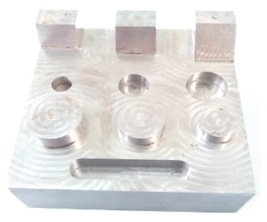
The metal piece that appears in Figure 1 has been the one targeted within this research for the measurements of Geometrical Product Specifications. The goal has been to analyze the influence of three parameters on three different levels on the accuracy of five variables (parallelism, angularity, roundness, diameter, and distance) described further on this paper.

Parallelism can be also specified as a tolerance zone defined by two parallel planes or lines parallel to a datum plane or axis, respectively, within where the surface or axis of the feature must lie [19]. Angularity tolerance specifies a tolerance zone defined by two parallel planes at the specified angle other than 90 degrees from a datum plane or axis within where the surface or the axis of the feature must lie [20].

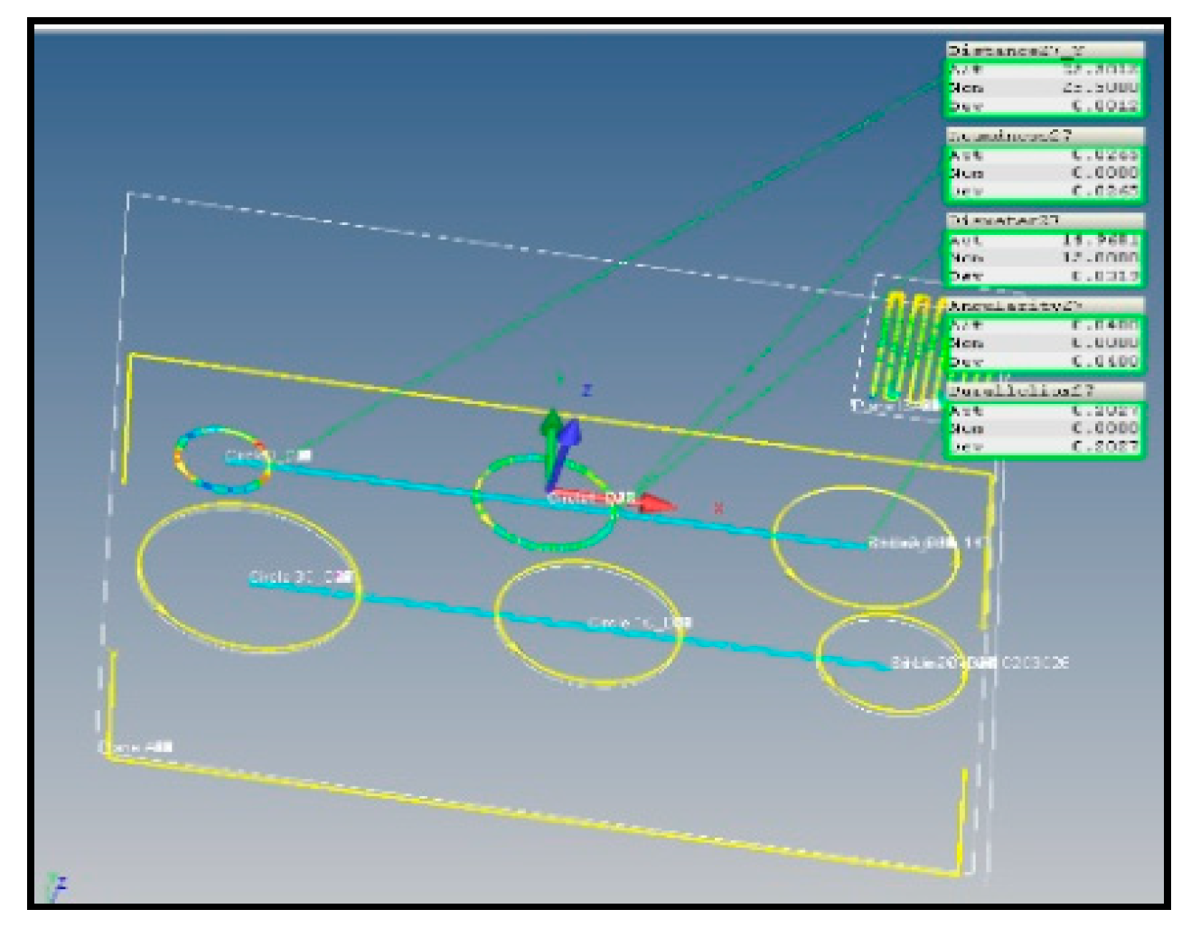
In the paper of [1], the authors mention that, according to the ISO12181-1, roundness tolerance is defined as the zone between two concentric circles which enclose the circular profile. Besides, it limits the roundness deviations, which is the distance between two concentric circles touching and enclosing the extracted circle (i.e., measured points) at the minimum radial distance from each other. The other two variables were diameter and distance between the centers of two circumferences. The software CALYPSO from ZEISS (Figure 2) was used for data evaluation.

2.3. The Coordinate Measuring Machines Used

The measurements and data acquisition were carried out by a single operator. Operator error was therefore eliminated from the measurement. In randomly chosen repeated measurement runs, a set of statistically significant values were obtained and used as input for further evaluation. A total of 81 readings were obtained.

The ZEISS CenterMax was used for obtaining all the data of this research that directly refer to the DOE and ANOVA mentioned before (Figure 3). This machine uses the tactile sensor VAST XTR gold, and possesses a mean percentage error (MPE) between 1.2 + L/280 and 2.2 + L/180 µm for temperatures ranging between 20 °C to 40 °C. In general terms, the CMM can operate in environment conditions ranging even from 8 °C to 40 °C, offering better stability in the measurements between +15 °C to +40 °C. The measurement within this study were all executed at room temperatures between 26 °C to 28 °C.

Sequence of steps for the realization of the experiment:

• Measuring plan programming in the CALYPSO software;
• Measurement of the part on ZEISS CenterMax to get data value;
• ANOVA to analyze and quantify the influence of the defined factors and their interaction on the measurement results.

3. Results and Discussion

The analysis of variance for the random model partition the total variability in the observations into a component that measures the variation between treatments (SS_Treatments) and a component that measures the variation within treatments (SSE). In this regard, the hypotheses tested refer to the variance component as it is shown next.

H0: ${\sigma }_{\mathrm{step}\mathrm{width}}^2=0$	H1:${\sigma }_{\mathrm{step}\mathrm{width}\ast \mathrm{stylus}\mathrm{tip}\ast \mathrm{speed}}^2>0$
H0: ${\sigma }_{\mathrm{stylus}\mathrm{tip}}^2=0$	H1:${\sigma }_{\mathrm{step}\mathrm{width}}^2>0$
H0: ${\sigma }_{\mathrm{speed}}^2=0$	H1: ${\sigma }_{\mathrm{stylus}\mathrm{tip}}^2>0$
H0: ${\sigma }_{\mathrm{step}\mathrm{width}\ast \mathrm{stylus}\mathrm{tip}}^2=0$	H1: ${\sigma }_{\mathrm{speed}}^2>0$
H0: ${\sigma }_{\mathrm{step}\mathrm{width}\ast \mathrm{speed}}^2=0$	H1: ${\sigma }_{\mathrm{step}\mathrm{width}\ast \mathrm{stylus}\mathrm{tip}}^2>0$
H0: ${\sigma }_{\mathrm{stylus}\mathrm{tip}\ast \mathrm{speed}}^2=0$	H1: ${\sigma }_{\mathrm{step}\mathrm{width}\ast \mathrm{speed}}^2>0$
H0: ${\sigma }_{\mathrm{step}\mathrm{width}\ast \mathrm{stylus}\mathrm{tip}\ast \mathrm{speed}}^2=0$	H1: ${\sigma }_{\mathrm{stylus}\mathrm{tip}\ast \mathrm{speed}}^2>0$

Before moving to the implementation of the ANOVA for this study, it was first necessary to determine if the ordinary least squares assumptions for all analyzed variables of Equation (1) were being met, i.e., homoscedasticity, normality, and independence. These assumptions are verified through the residual plots that are presented below. As an example, the behavior of the assumptions in the variable parallelism will be explained in detail. The residual histogram is an exploratory tool to prove the general characteristics of the data. Figure 4 shows that the data is not skewed and there are no outliers.

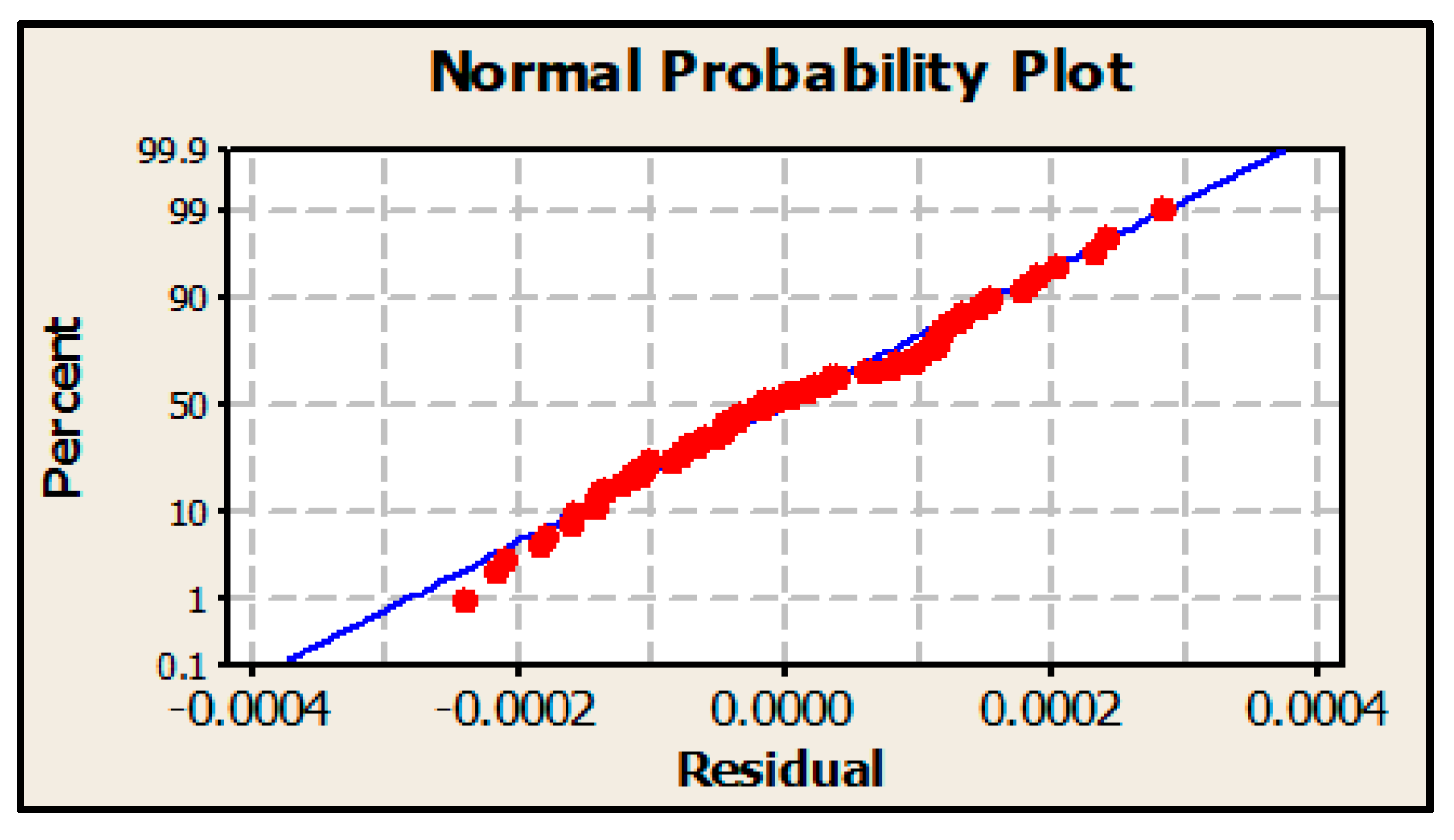
The normal probability plot of the residuals for this experiment is shown in Figure 5. The points in this plot represent a straight line that verifies the assumption that the residuals are normally distributed.

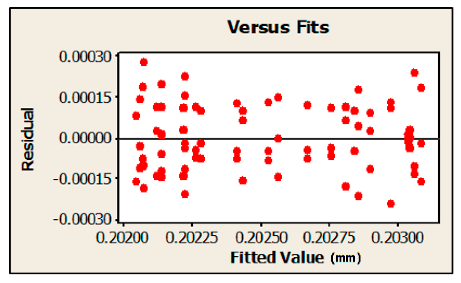
The residuals in Figure 6 versus fits shows a random order of residuals on both sides of line 0. It has a constant variation without any recognizable patterns in the residual plot.

The residuals versus order plot shows all residuals in the order that the data was collected and used to find non-random error, especially of time-related effects. Figure 7 shows that the residuals are not correlated with each other.

In the same way, the fulfillment of the assumptions was verified in the rest of the variables analyzed (angularity, roundness, diameter, and distance); these plots are all shown in Figure 8. Notice, however, that the software does allow adding units to the plots between Figure 4 and Figure 7 given that this is not considered necessary; however, for the sake of comprehension, the authors did want to specify this on the residual versus fits plot.

Subsequently, an ANOVA was applied using the Minitab 16 software to determine whether the predictors or factors are significantly related to the response. The mean square (MS), F-, and p-values can be observed in

Table 3. Summary of key analysis of variance (ANOVA) values for each of the variables Parallelism, Angularity and Roundness.

	Parallelism			Angularity			Roundness
Source	MS	F	p-Value	MS	F	p-Value	MS	F	p-Value
Stylus diameter	3.78 × 10−6	22.81	0.000	8.27 × 10−4	43.59	0.001	7.94 × 10−6	0.56	0.599
Step width	3.78 × 10−6	1.32	0.385	7.06 × 10−5	3.71	0.108	4.18 × 10−5	1.92	0.223
Speed	1.1 × 10−6	6.35	0.000	2.52 × 10−5	0.91	0.451	8.75 × 10−5	4.20	0.071
Stylus diameter*Step width	1.5 × 10−8	0.45	0.586	7.15 × 10−6	1.82	0.218	8.46 × 10−6	5.08	0.025
Stylus diameter*Speed	1.52 × 10−7	4.61	0.000	1.58 × 10−5	4.01	0.045	7.48 × 10−6	4.49	0.034
Step width*Speed	2.6 × 10−8	0.79	0.325	1.58 × 10−5	4.03	0.044	1.50 × 10−5	9.02	0.005
Stylus diameter*Step width*Speed	3.3 × 10−8	1.57	0.167	3.93 × 10−6	26.70	0.023	1.67 × 10−6	40.63	0.000
Error	2.1 × 10−8			1.47 × 10−7			4.10 × 10−8

and

Table 4. Summary of key analysis of variance (ANOVA) values for each of the variables Diameter and Distance.

	Diameter			Distance
Source	MS	F	p-Value	MS	F	p-Value
Stylus diameter	4.68 × 10−5	39.39	0.000	1.27 × 10−5	1.01	0.438
Step width	3.79 × 10−6	0.47	0.657	1.59 × 10−5	2.06	0.260
Speed	1.46 × 10−5	1.84	0.275	9.53 × 10−6	0.79	0.513
Stylus diameter*Step width	6.73 × 10−7	1.00	0.458	5.89 × 10−6	1.63	0.257
Stylus diameter*Speed	5.33 × 10−7	0.79	0.557	1.03 × 10−5	2.85	0.097
Step width*Speed	8.11 × 10−6	12.06	0.000	5.43 × 10−6	1.51	0.287
Stylus diameter*Step width*Speed	6.72 × 10−7	134.40	0.000	3.60 × 10−6	78.3	0.000
Error	5.00 × 10−9			4.60 × 10−8

. These tables have been prepared as a summary containing the values obtained for each of the variables studied.

For those cases where the p-value is less than the level of significance α (0.05), it is concluded that the corresponding hypothesis is significant; that is, this effect is active or does influence the response variable. Similarly, whenever it is concluded that an interaction between factors has a statistically important effect on the response, its interpretation takes precedence over the corresponding main effects, although these are also significant. This is because when the interaction is significant, it governs the behavior of the response in the function of such factors.

Under these premises, Table 3 and Table 4 show key ANOVA values for all the variables under study.

Based on the p-values from thesetables, especially those in bold, it is possible to conclude that the Stylus diameter*Step width*Speed effects are active at a confidence level of 95% (value of p < 0.05). Similarly, a strong contribution of the interaction between Stylus diameter*Step width in the error of the average measurement of the roundness is also showed. Besides, the interaction between the factors Stylus diameter*Speed influences the measurements of the variable’s parallelism, angularity, and roundness. The interaction between Step width*Speed is active for angularity, roundness, and diameter. As for the main effects, the Stylus diameter is the most active with the most influence on the variability of the Geometrical Product Specifications.

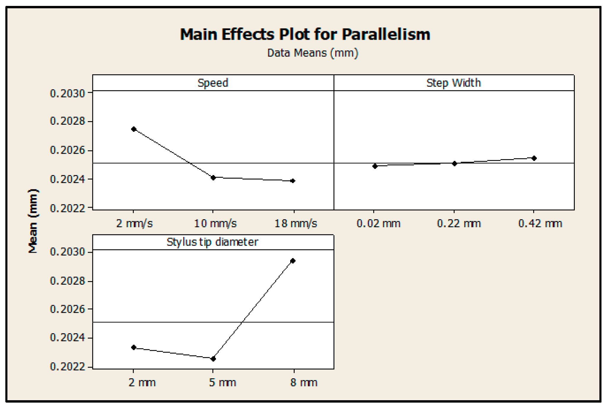
To further assist in the practical interpretation of this experiment, Figure 9 presents plots of the three main effects. The main effect occurs when the mean response changes across the levels of a factor. These main effect plots are graphs of the marginal response averages at the levels of the three factors. Thus, in this case, the plot has been obtained by plotting the means for each value of a categorical variable. By analyzing the line linking the points, it is possible to determine whether the main effect is present for a categorical variable or not. The plots also exhibit another reference line that shows the overall mean of all measurements.

When the reference line is horizontal (parallel to the x-axis), there is no main effect present. The response mean is the same across all factor levels. This particular situation occurs with the factor Step width, which shows that, for the analysis of the variable parallelism, the variation existing in the three levels studied (0.02, 0.22, 0.42) is not significant.

On the other hand, when the line is not horizontal, there is a main effect present and the response mean is not the same across all factor levels. In this situation, the steeper the slope of the line, the greater the magnitude of the main effect. In this regard, it is also possible to see from the plot that the three variables have no positive main effects; that is, the plots do not show that by increasing or decreasing a variable’s level, the average deviation necessarily increases or decreases all the time.

In this regard, the analysis of the Speed factor shows a non-linear behavior. In this case, the highest value of the average is obtained at the level of 2 mm/s. For the remaining levels, the average value drops by around 4 µm. A similar analysis can be used for the Stylus diameter factor; however, this has an inverse behavior. In this case, the maximum average value is reached during the use of the third factor´s level, i.e., Stylus diameter of 8 mm, representing a difference of up to 8 µm over the average mean value. These results in the plot once more confirm the outcome and conclusions obtained in the ANOVA table where both factors turned out to be significant in the measurement variability of the variable parallelism.

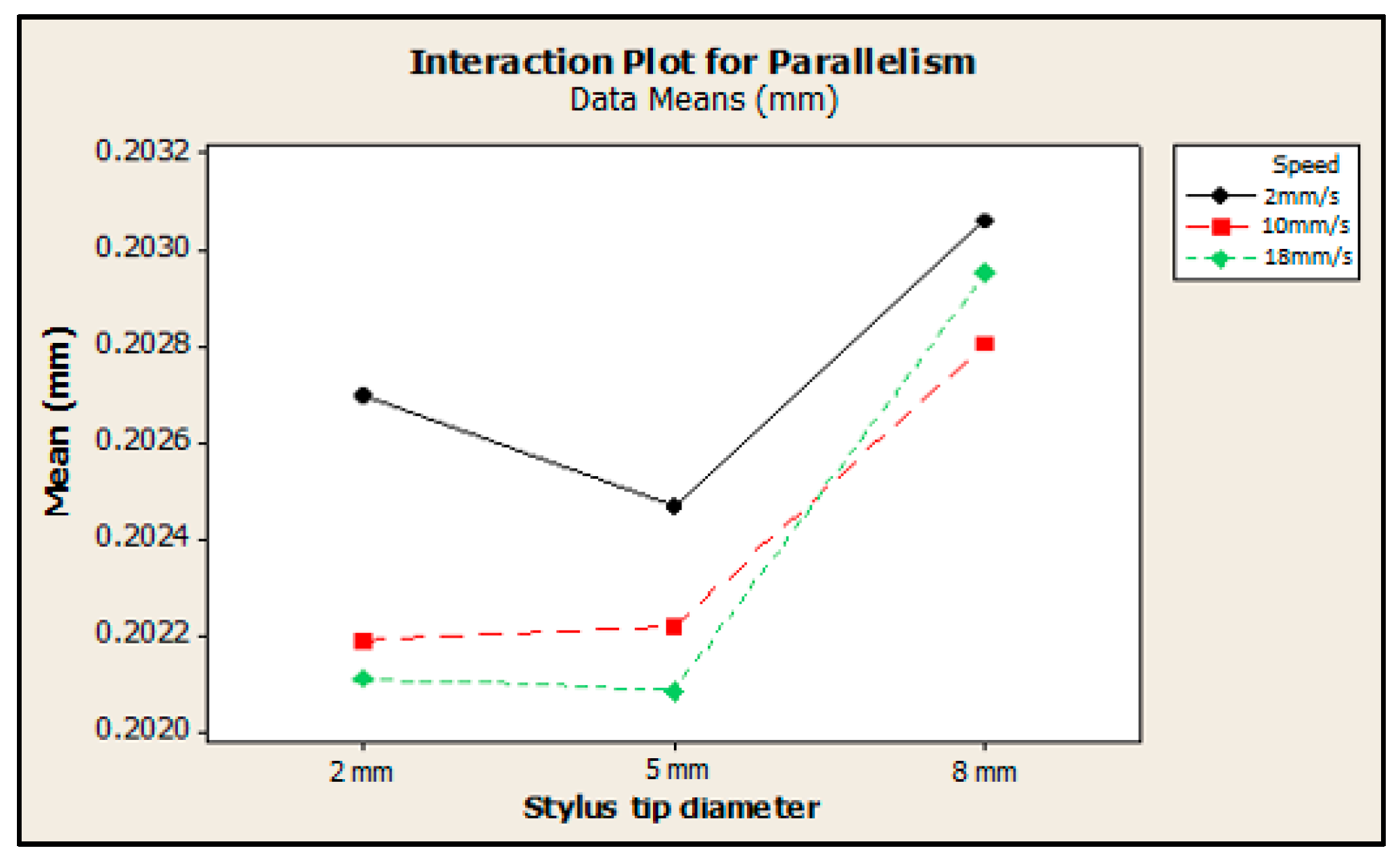
On the other hand, Figure 10 shows the interaction between the factors Stylus diameter and Speed on the variable parallelism as an illustrative example. This was selected because it was statistically significant in the 95% confidence interval in the ANOVA table. The significant interaction is indicated by the lack of parallelism of the lines. In general, the behavior of the average varies depending on the interaction of both factors implying that when the measuring Speed is the same, different values will be obtained depending on the Stylus diameter these are measured with. For example, maintaining a constant Speed of 18 mm/s and varying the Stylus diameter from 2 mm to 8 mm yields a measurement value that differs in up to 8 µm with respect to the initial Stylus diameter level. At the same time, when using the same Stylus diameter, e.g., 2 mm, it is possible to see how changing the Speed of the measurement leads to obtaining three different values that range from 0.2021 mm to 0.2027 mm.

As stated in [16], the accuracy indicates the relative closeness of agreement between an experimentally determined value of a quantity and its true value. Standard uncertainties are the difference between the experimentally determined value and truth; thus, as error decreases, accuracy is said to increase. Only in rare instances is the true value of quantity known. Uncertainty (U) estimate, for example, means that the true value of the quantity is expected to be within the ±U interval about the experimental value.

An analysis of measurement uncertainty that uses components of variance turns out to be an appropriate estimator for the evaluation of Geometrical Product Specifications measurement uncertainty on CMMs. In this regard,

Table 5. Coordinate measuring machine (CMM) measurement uncertainty analysis (µm).

Source	Parallelism	Angularity	Roundness	Diameter	Distance
Stylus diameter	1.82	8.73	0.00	6.63	0.00
Step width	1.92	2.38	0.00	0.00	0.00
Speed	0.77	0.00	4.66	0.00	0.00
Stylus diameter*Step width	0.00	1.80	2.61	0.03	1.51
Stylus diameter*Speed	0.34	3.44	2.41	0.00	2.58
Step width*Speed	0.00	3.45	3.65	2.73	1.35
Stylus diameter*Step width*Speed	0.06	1.12	0.74	0.47	1.09

shows the results of the uncertainty analysis attributed to factors and their interaction. The standard uncertainties of the Stylus diameter, Step width, and Speed variables were determined according to Equations (14)–(16), respectively, while the standard uncertainty of the subsequent interactions was also determined according to Equations (17)–(20), in this particular order.

The highest values of uncertainty given by the factors and their interactions on the measurement of Geometrical Product Specifications are indicated in bold in Table 5. From the results appearing in this table, it can be concluded that the standard uncertainties of the machine associated with the factors Stylus diameter, the Step width, and the Speed do influence some of the variables being evaluated. For example, the highest value of the standard uncertainty is associated with the Stylus diameter in the evaluation of angularity and diameter. This means that any change related to this factor, i.e., a change related to its random levels, would influence the uncertainty in a value that reaches the up to 8.73 µm and 6.63 µm, respectively.

Similarly, the effect of the Step width on the angularity evaluation is represented by an uncertainty value of 2.38 µm. If there is a limit or tolerance set for the angularity higher than 3 µm, it would not be necessary to deal with the Step width set up; however, in this particular case, it is also important to take into consideration that the same Stylus diameter would be also bringing higher uncertainty for the analyzed variable.

In the case of the Speed factor, it has the biggest influence on the measurement and evaluation of a form parameter (roundness). The other evaluated variables were not affected by this factor. This finding is especially significant and could lead to higher productivity in terms of the dimensions’ evaluation because it allows using higher values of scanning speed than the ones in the Cookbook suggested for the measurement and evaluation of features.

It is also important to notice that the lowest uncertainty values (italicized in the table) are those related to maximal accuracy.

4. Conclusions

The present paper addressed the important topic of uncertainty analysis in the case of CMM. The main goal aimed at analyzing and quantifying the influence of key factors and their interactions on the measurements’ uncertainty of defined variables. The paper started with an analysis of related literature and subsequently proceeded to the design and implementation of a Random Factorial Design of Experiments that took into consideration factors like the Stylus diameter, Step width, and Speed, using three levels each.

The investigation allowed estimating the uncertainty of the CMM measurement using statistical methods such as the DOE with random factors and the ANOVA. The application made in the measurement of five variables (parallelism, angularity, roundness, diameter, and distance) offered relevant information on the performance of the CMM and its accuracy based on the variation of the studied factors through their random levels. The ANOVA results showed a strong interaction among the factor Stylus diameter, Step width, and Speed, meaning that a noticeable variation in the mean measurement error was generated when changing the levels of these factors simultaneously.

The highest value of standard uncertainty was associated with the Stylus diameter of 8 mm in the evaluation of the variable’s angularity and diameter. In this case, it meant that any change related to its levels would influence the uncertainty in a value that could reach up to 8.73 µm and 6.63 µm, respectively. In the case of the Speed factor, it has the biggest influence on the measurement and evaluation of a form parameter (roundness) reaching up to 4.66 µm.

The findings and results obtained by the experimental investigation can be taken as a reference for more optimized use of the factor and their levels in the measurement of the Geometrical Products Specifications under question, and this in order to face lesser values of the uncertainty. In practical terms, these results can be used, for example, to reduce the time spent in the measurements that leads to increased productivity in the measuring of Geometrical Products Specifications, e.g., by using higher speeds in the scanning of the measured part.

In the end, besides all previous elements, the authors believe this paper contributes to a better and more flexible use and comprehension of the factors, their interactions, and the variables analyzed, all this in the context of the ZEISS CenterMax CMM.