Characteristic Length and Time Scales of the Highly Forward Scattering of Photons in Random Media

Abstract

Background: Elucidation of the highly forward scattering of photons in random media such as biological tissue is crucial for further developments of optical imaging using photon transport models. We evaluated length and time scales of the photon scattering in three-dimensional media. Methods: We employed analytical solutions of the time-dependent radiative transfer, M-th order delta-Eddington, and photon diffusion equations (RTE, dEM, and PDE). We calculated the fluence rates at different source-detector distances and optical properties. Results: We found that the zeroth order dEM and PDE, which approximate the highly forward scattering to the isotropic scattering, are valid in longer length and time scales than approximately $10/{\mu }_t^{\prime }$ and $40/{\mu }_t^{\prime }v$, respectively, where ${\mu }_t^{\prime }$ is the reduced transport coefficient and v the speed of light in a medium. The first and second order dEM, which approximate the highly forward-peaked phase function by the first two and three Legendre moments, are valid in the longer scales than approximately $4.0/{\mu }_t^{\prime }$ and $6.3/{\mu }_t^{\prime }v$; $2.8/{\mu }_t^{\prime }$ and $3.5/{\mu }_t^{\prime }v$, respectively. The boundary conditions less influence the length scales, while they reduce the times scales from those for bulk at the longer length scale than approximately $4.0/{\mu }_t^{\prime }$. Conclusion: Our findings are useful for constructions of accurate and efficient photon transport models. We evaluated length and time scales of the highly forward scattering of photons in various kinds of three-dimensional random media by analytical solutions of the radiative transfer, M-th order delta-Eddington, and photon diffusion equations.

1. Introduction

Elucidation of the photon scattering and transport in random media such as biological tissue volumes is crucial for biomedical optical imaging using the near-infrared light in the wavelength range from 700 to 1100 nm such as diffuse optical tomography [1,2,3], because the imaging technique uses light scattered by the media. There are mainly three kinds of systems of the imaging techniques: time-domain, steady-state, and frequency-domain systems. Among them, the time-domain system has several advantages over steady-state and frequency-domain systems thanks to the richest information of the time-domain measurement data [4]. Time-dependent photon transport is basically classified into the two kinds of characteristic regimes (length and time scales): the ballistic and diffusive regimes corresponding to short and long source-detector (SD) distances and times after light incidence, respectively [5]. In the ballistic regime, photon is little scattered and almost goes straight. In the diffusive regime, photon is diffusive due to multiple scattering of photons, and the scattering process can be approximated as isotropic. Between the ballistic and diffusive regimes, photon undergoes a few scattering events in the highly forward direction and travels along the zig-zag paths while changing the direction [6,7]. In this paper, we call this few-scattering-event regime between the ballistic and diffusive regimes as the scattering regime, so that we consider the three kinds of characteristic regimes for photon transport. The radiative transfer equation (RTE), which is the linear Boltzmann equation, can describe photon transport for random media in the three characteristic regimes because the phase function in the RTE can treat the highly forward scattering of photons. However, the numerical calculations of the RTE require high computational loads (times and memories) especially for three-dimensional (3D) random media because the RTE is an integro-differential equation with respect to the light intensity as a function of position vector, unit angular direction vector, and time. To reduce the computational loads, many researches have employed the photon diffusion equation (PDE), which is obtained by the diffusion approximation to the RTE and omits the angular direction. However, the PDE is valid only in the diffusive regime. A coupling model using the RTE and PDE has been constructed [8,9]. For the coupling model, the RTE is calculated in the ballistic and scattering regimes, while the PDE is calculated in the diffusive regime. For constructions of the coupling model or appropriate uses of the PDE, many researches have devoted their work to evaluations of the crossover length and time from the scattering to diffusive regimes [9,10,11,12,13,14,15]. For example, a comparison study [10] between actual light measurements and the PDE-results for slab media showed that the crossover length is evaluated as approximately 10/${\mu }_t^{\prime }$, where the reduced transport coefficient ${\mu }_t^{\prime }$ is a sum of reduced scattering coefficient and absorption coefficient. A numerical study [9] using the time-dependent RTE and PDE for 2D media evaluated the crossover length the same as the above study [10], and in addition, evaluated the crossover time as approximately 20/${\mu }_t^{\prime }v$, where v is the speed of light in the medium. Although the coupling model can provide accurate and efficient results, a further efficiency improvement of the photon transport model is necessary because the RTE-calculations in the scattering regime still require high computational loads. For modeling the highly forward scattering of photons, the phase function in the RTE is highly forward-peaked and changes exponentially with respect to the scattering angle. Basically, accurate numerical treatments of the highly forward-peaked phase function require a large number of discrete angular directions, resulting in high computational loads of the RTE-calculations. To overcome the difficulty, one needs to investigate the highly forward scattering of photons and influences of the highly forward-peaked phase function on the RTE-results in the scattering regime. For this purpose, in this paper, we employ the M-th order delta-Eddington equation (dEM), which is obtained by the delta-Eddington approximation (dEA) to the RTE.

The dEA decomposes the highly forward-peaked phase function into purely forward-peaked and other components [16,17]. The purely forward-peaked component is given by the delta-function and contributes to a modification of the scattering length scale. The other components are expanded by finite series of Legendre polynomials and used as the phase function in the dEM. The dEM has been widely employed in the field of biomedical optics since Klose and coworkers have introduced from the field of astrophysics [18,19,20,21,22]. It has been shown that the numerical solutions of the dEM agree with those of the RTE while the number of the discrete angular directions is reduced to approximately one-sixth of the required number for the RTE-calculations. Nevertheless, a validity of the dEM is still unclear; Klose and coworkers showed that the second order dEM can provide the accurate results the same as the RTE [21], while Jia and coworkers stated that the zeroth order dEM is sufficient [22], and Boulet and coworkers employed the zeroth and first order dEM [20]. These differences probably come from the fact that the validity of the dEM depends on the SD distances, times after light incidence, and the optical properties, like the validity of the PDE.

Our objective is to examine photon transport especially in the scattering regime for various kinds of random media by using the time-dependent RTE, dEM, and PDE, and to evaluate a regime (length and time scales) for the dEM to be valid as a function of ${\mu }_t^{\prime }$ and ${\mu }_t^{\prime }v$. We employed the analytical solutions instead of the numerical solutions because the analytical solutions are attained much faster than the numerical solutions and allow us to investigate a wide range of the SD distances and optical properties. In addition, we can focus the modification of the scattering coefficient and the approximation of the phase function by the dEA without a discussion of numerical errors induced by the numerical discretization. To the best of our knowledge, no studies have reported to evaluate the regime for the dEM. In this paper, we investigate photon transport for infinite and semi-infinite 3D homogeneous media as a first step of investigations for realistic heterogeneous biological tissue volumes. The investigations for infinite and semi-infinite 3D homogeneous media have been widely discussed for the diffuse optics community [4]. The analytical solutions have been employed for evaluations of the optical properties of various kinds of random media such as biological tissue volumes, colloidal suspensions [23], and agricultural products [24]. The following section describes the three kinds of the photon transport models for 3D random media: the time-dependent RTE, dEM, and PDE; and analytical solutions of the three models for the temporal profiles of the fluence rate. Section 3 investigates the results of the analytical solutions and evaluates the regime for the dEM. Finally, conclusions are described.

2. Materials and Methods

2.1. Time-Domain Photon Transport Models

2.1.1. Radiative Transfer Equation (RTE)

We consider photon transport in the length and time scales of the mean free path and mean time of flight. Then, photon transport can be described by the RTE [25]. For 3D random media, the time-dependent RTE is given by

$$\left[\frac{\partial }{v\partial t}+\mathsf{\Omega }·\mathbf{\nabla }+{\mu }_a\left(\mathit{r}\right)+{\mu }_s\left(\mathit{r}\right)\right]I(\mathit{r},\mathsf{\Omega },t)={\mu }_s\left(\mathit{r}\right){\int }_{{\mathbb{S}}^2}d{\mathsf{\Omega }}^{\prime }p(\mathsf{\Omega },{\mathsf{\Omega }}^{\prime })I(\mathit{r},{\mathsf{\Omega }}^{\prime },t)+q(\mathit{r},\mathsf{\Omega },t),$$

(1)

where, $I(\mathit{r},\mathsf{\Omega },t)$ in $\mathrm{W}{\mathrm{cm}}^{-2}{\mathrm{sr}}^{-1}$ represents the light intensity as a function of spatial position vector $\mathit{r}=(x,y,z)\in {\mathbb{R}}^3$ in $\mathrm{cm}$; angular direction (unit direction vector) $\mathsf{\Omega }=({\mathsf{\Omega }}_x,{\mathsf{\Omega }}_y,{\mathsf{\Omega }}_z)\in {\mathbb{S}}^2$ in sr; and time t in ps. ${\mu }_a\left(\mathit{r}\right)$ and ${\mu }_s\left(\mathit{r}\right)$ in ${\mathrm{cm}}^{-1}$ are the absorption and scattering coefficients, respectively; v is the speed of light in the medium; $p(\mathsf{\Omega },{\mathsf{\Omega }}^{\prime })$ in ${\mathrm{sr}}^{-1}$ is the phase function with $\mathsf{\Omega }$ and ${\mathsf{\Omega }}^{\prime }$ denoting the scattered-out and -in directions, respectively; and $q(\mathit{r},\mathsf{\Omega },t)$ in $\mathrm{W}{\mathrm{cm}}^{-3}{\mathrm{sr}}^{-1}$ is a source function.

2.1.2. Henyey-Greenstein Phase Function and Anisotropy Factor

For a formulation of $p(\mathsf{\Omega },{\mathsf{\Omega }}^{\prime })$, the Henyey-Greenstein (HG) phase function [26] is widely employed in biomedical optics to model the forward scattering of photons:

$$p_{HG}(\mathsf{\Omega }·{\mathsf{\Omega }}^{\prime })=\frac{1}{4\pi }\frac{1-g^2}{{\left(1+g^2-2g\mathsf{\Omega }·{\mathsf{\Omega }}^{\prime }\right)}^{3/2}},$$

(2)

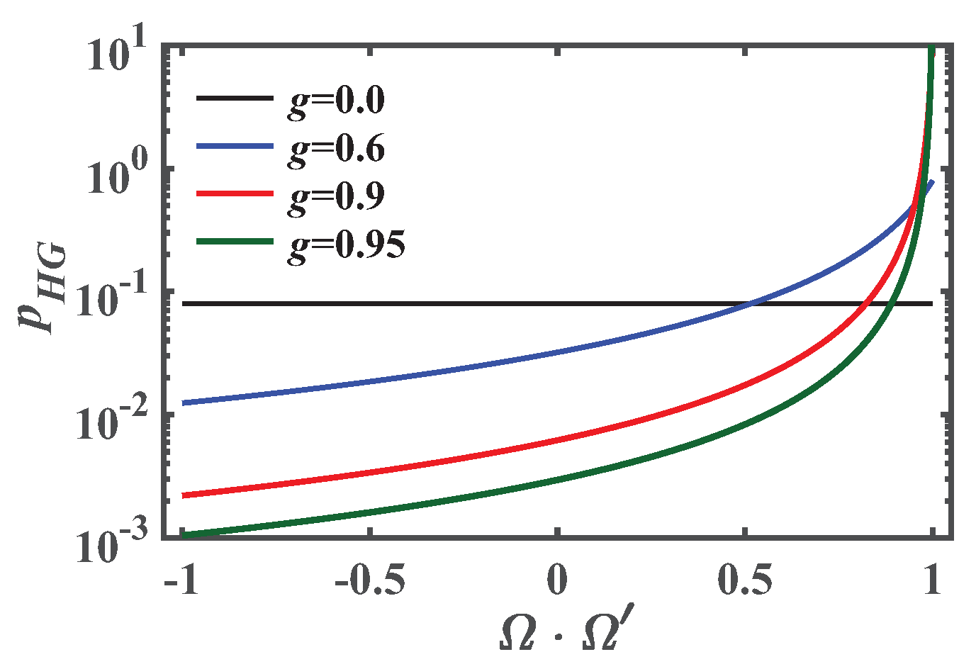
where $g\in$[−1, 1] is the anisotropy factor, defined by ${\int }_{{\mathbb{S}}^2}d{\mathsf{\Omega }}^{\prime }(\mathsf{\Omega }·{\mathsf{\Omega }}^{\prime })p(\mathsf{\Omega },{\mathsf{\Omega }}^{\prime })$. Mostly, g-values of biological tissue volumes are larger than 0.8 [27], meaning the highly forward scattering. For examples, the g-value of muscle or bone is considered as 0.9; and the g-values of the human liver and of blood vessels are 0.955 [28] and 0.992 [29], respectively. Meanwhile, there are void regions in the human body such as the trachea in the human neck, whose g-value is almost zero, meaning the isotropic scattering. Figure 1 shows the HG phase function (Equation (2)) as a function of $\mathsf{\Omega }·{\mathsf{\Omega }}^{\prime }\in [-1,1]$ in a logarithmic scale. At $g=0.0$ (isotropic scattering), the phase function is constant over the whole region of $\mathsf{\Omega }·{\mathsf{\Omega }}^{\prime }$. Meanwhile, as the g-value approaches to unity from zero (enhancement of the highly forward scattering), the exponential change of $p_{HG}$ with respect to $\mathsf{\Omega }·{\mathsf{\Omega }}^{\prime }$ becomes large and the peak of $p_{HG}$ around $\mathsf{\Omega }·{\mathsf{\Omega }}^{\prime }=1.0$ becomes sharp.

The HG phase function is expanded in the infinite series of (unassociated) Legendre polynomials $P_l$ ($l=0,1,\cdots ,\infty$):

$$p_{HG}(\mathsf{\Omega }·{\mathsf{\Omega }}^{\prime })=\sum _{l=0}^{\infty }\frac{2l+1}{4\pi }{g}^l{P}_l(\mathsf{\Omega }·{\mathsf{\Omega }}^{\prime }),$$

(3)

where $g^l$ is the l-th order expansion coefficient.

2.1.3. M-th Order Delta-Eddington Equation (dEM)

The dEA decomposes the highly forward-peaked phase function into a purely forward-peaked component expressed by the delta function and the other components [16,17]:

$$p_{\delta }^M(\mathsf{\Omega }·{\mathsf{\Omega }}^{\prime })=\frac{1}{2\pi }h\delta (1-\mathsf{\Omega }·{\mathsf{\Omega }}^{\prime })+(1-h)p_{\delta 2}^M(\mathsf{\Omega }·{\mathsf{\Omega }}^{\prime }),$$

(4)

where h is a coefficient of the decomposition. $p_{\delta 2}^M$ is a phase function excluding the delta-function component and expanded in the finite series of Legendre polynomials up to the order of M:

$$p_{\delta 2}^M(\mathsf{\Omega }·{\mathsf{\Omega }}^{\prime })=\sum _{l=0}^M\frac{2l+1}{4\pi }{\sigma }_{dEl}{P}_l(\mathsf{\Omega }·{\mathsf{\Omega }}^{\prime }).$$

(5)

In the case of the HG phase function, the expansion coefficient ${\sigma }_{dEl}$ and the decomposition coefficient h are determined so as to satisfy the moment conditions up to the order of $M+1$:

$${\sigma }_{dEl}:={\int }_{{\mathbb{S}}^2}d{\mathsf{\Omega }}^{\prime }{p}_{\delta 2}^M(\mathsf{\Omega }·{\mathsf{\Omega }}^{\prime })P_l(\mathsf{\Omega }·{\mathsf{\Omega }}^{\prime })=\frac{g^l-h}{1-h},h=g^{M+1}.$$

(6)

The case of $l=0$ in Equation (6) corresponds to the normalization condition of $p_{\delta 2}^M$: ${\int }_{{\mathbb{S}}^2}d{\mathsf{\Omega }}^{\prime }{p}_{\delta 2}^M(\mathsf{\Omega }·{\mathsf{\Omega }}^{\prime })=1$. By using $p_{\delta }^M$ (Equation (4)), the RTE (Equation (1)) is approximated to

$$\left[\frac{\partial }{v\partial t}+\mathsf{\Omega }·\mathbf{\nabla }+{\mu }_a\left(\mathit{r}\right)+{\mu }_s^M\left(\mathit{r}\right)\right]I(\mathit{r},\mathsf{\Omega },t)={\mu }_s^M\left(\mathit{r}\right){\int }_{{\mathbb{S}}^2}d{\mathsf{\Omega }}^{\prime }{p}_{\delta 2}^M(\mathsf{\Omega }·{\mathsf{\Omega }}^{\prime })I(\mathit{r},{\mathsf{\Omega }}^{\prime },t)+q(\mathit{r},\mathsf{\Omega },t),$$

(7)

where ${\mu }_s^M\left(\mathit{r}\right)=(1-h){\mu }_s\left(\mathit{r}\right)=(1-g^{M+1}){\mu }_s\left(\mathit{r}\right)$. In this paper, Equation (7) is called as the M-th order delta-Eddington equation (dEM). Comparing the RTE (Equation (1)) with the dEM, ${\mu }_s$ is modified to ${\mu }_s^M$ and p is approximated to $p_{\delta 2}^M$. The modification of ${\mu }_s$ to ${\mu }_s^M$ means a change of the scattering length scale. Figure 2a,b plot a scattering length ratio of ${\mu }_s^M/{\mu }_s$ and a relative error $E_{phase}^M$ of the phase functions between the HG function (Equation (2)) and the M-th order dEA (Equation (5)) at different g-values of 0.3, 0.6, 0.9, and 0.95. Here, the error $E_{phase}^M$ is defined by

$$E_{phase}^M={\int }_{-1}^{1}d\mu \left|\frac{p_{\delta 2}^M\left(\mu \right)-p_{HG}\left(\mu \right)}{p_{HG}\left(\mu \right)}\right|,\mu =\mathsf{\Omega }·{\mathsf{\Omega }}^{\prime }.$$

(8)

As the expansion order M increases, the ratio ${\mu }_s^M/{\mu }_s$ approaches to unity and the error $E_{phase}^M$ decreases, meaning the scattering length scale and the phase function for the dEM converge to those for the RTE. At $g=0.9$ and 0.95 (highly forward scattering), the convergences are slower than the cases of $g=0.3$ and 0.6 (moderate forward scattering).

2.1.4. Photon Diffusion Equation (PDE)

The PDE is obtained by the diffusion approximation to the RTE [30]:

$$\left[\frac{\partial }{v\partial t}-\mathbf{\nabla }·D\left(\mathit{r}\right)\mathbf{\nabla }+{\mu }_a\left(\mathit{r}\right)\right]\mathsf{\Phi }(\mathit{r},t)=q_{DE}(\mathit{r},t),$$

(9)

where the fluence rate $\mathsf{\Phi }(\mathit{r},t)$ is defined by ${\int }_{{\mathbb{S}}^2}d\mathsf{\Omega }I(\mathit{r},\mathsf{\Omega },t)$; the diffusion coefficient $D\left(\mathit{r}\right)$ is by $\left[3(1-g){\mu }_s\left(\mathit{r}\right)\right){]}^{-1}$; and the isotropic source $q_{DE}(\mathit{r},t)$ is by ${\int }_{{\mathbb{S}}^2}d\mathsf{\Omega }q(\mathit{r},\mathsf{\Omega },t)$.

2.2. Analytical Solutions (AS) of the Time-Domain Photon Transport Models

2.2.1. 3D Infinite Homogeneous Media

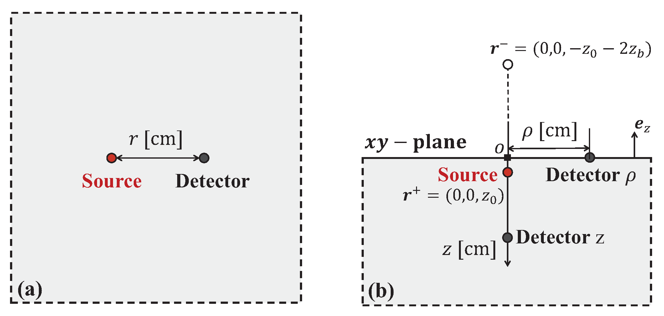
In this paper, we mainly employed the analytical solutions of the time-dependent RTE, dEM, and PDE for 3D infinite homogeneous media to calculate the temporal profiles of the fluence rate $\mathsf{\Phi }(\mathit{r},t)$ when an isotropic point source is incident at the initial time and at the origin of the $xyz$-coordinate as shown in Figure 3a. Then, the source-detector (SD) distance $r_{sd}$ is given by $r=\left|\mathit{r}\right|$. The analytical form of the fluence rate for the RTE ${\mathsf{\Phi }}_{RTE}(r,t)$ with an arbitrary g-value is derived by Liemert and Kienle [31]:

$${\mathsf{\Phi }}_{RTE}(r,t)={\mathsf{\Phi }}_{LK}(r,t;{\mu }_a,{\mu }_s,{\mathbf{\sigma }}_{\mathit{HG}},n),$$

(10)

where ${\mathsf{\Phi }}_{LK}$ represents the analytical form by Liemert and Kienle; ${\mathbf{\sigma }}_{\mathit{HG}}$ the vector of the expansion coefficients for the HG phase function up to a maximum order of N: $[1,g,g^2,g^3,\cdots ,g^N]$; the N-value is determined so as to attain sufficient convergence of the results; and n is the refractive index of the medium. The verifications of ${\mathsf{\Phi }}_{RTE}(r,t)$ were confirmed by several independent works [23,32]. Using ${\mathsf{\Phi }}_{LK}$, we can obtain the analytical form for the dEM ${\mathsf{\Phi }}_{dEM}(r,t)$:

$${\mathsf{\Phi }}_{dEM}(r,t)={\mathsf{\Phi }}_{LK}(r,t;{\mu }_a,{\mu }_s^M,{\mathbf{\sigma }}_{\mathbf{M}},n),$$

(11)

where ${\mathbf{\sigma }}_{\mathit{M}}$ represents the vector of the expansion coefficients for $p_{\delta 2}^M$ (Equation (6)) up to N$(>M)$: $[1,{\sigma }_{dE1},{\sigma }_{dE2},\cdots {\sigma }_{dEM},{\sigma }_{dEM+1}=0,\cdots ,{\sigma }_{dEN}=0]$. We confirmed the verification of ${\mathsf{\Phi }}_{dEM}(r,t)$ by comparing with the numerical solutions in Appendix A. The analytical solution for the dE0 ($M=0$) by Liemert and Kienle is largely oscillated and unstable for several cases such as short SD distances, short times after light incidence, and the low scattering coefficient. In those cases, we employed the analytical solution for the dE0 derived by Paasschens [33] instead. It is noted that Martelli and coworkers employed a heuristic approach to obtain the approximate solution of the RTE for highly forward scattering [34] from the exact solution of the RTE for isotropic scattering by Paasschens [33]. Their approach is identical to the zeroth order dEA, so that the $\mathsf{\Phi }(r,t)$-result using their approach coincides with the result of ${\mathsf{\Phi }}_{dE0}(r,t)$. The analytical form for the PDE ${\mathsf{\Phi }}_{PDE}(r,t)$ is given as [35]

$${\mathsf{\Phi }}_{PDE}(r,t)=\frac{1}{{\left(4\pi Dt\right)}^{3/2}}exp\left[-{\mu }_{a}vt-\frac{r^2}{4Dvt}\right].$$

(12)

2.2.2. 3D Semi-Infinite Homogeneous Media

To investigate influences of the boundary conditions on the temporal profiles of the fluence rate, we employed the approximate solutions of the RTE, dEM, and PDE for 3D semi-infinite homogeneous media under the diffusive refractive-index mismatched boundary condition:

$$\mathsf{\Phi }(\mathit{r},t)+D\gamma \left(n\right){\mathit{e}}_z·\mathbf{\nabla }\mathsf{\Phi }(\mathit{r},t)=0,$$

(13)

where ${\mathit{e}}_z$ represents the outward normal unit vector at the $xy$-plane in Figure 3b, the coefficient $\gamma \left(n\right)$ is give by $2(1+R_f)/(1-R_f)$ with $R_f=-1.44n^{-2}+0.71n^{-1}+0.69+0.064n$ [36]. Using the extrapolation method for the boundary condition (Equation (13)) [37], the analytical solutions of the RTE, dEM, and PDE for semi-infinite homogeneous media are obtained:

$${\mathsf{\Phi }}_{semi}(\mathit{r},t;z_0,z_b)={\mathsf{\Phi }}_{inf}\left(\right|\mathit{r}-{\mathit{r}}^{+}|,t)-{\mathsf{\Phi }}_{inf}\left(\right|\mathit{r}-{\mathit{r}}^{-}|,t),$$

(14)

where $\mathit{r}=(\mathbf{\rho },z)$, $\mathbf{\rho }=(x,y)$, a real source position of ${\mathit{r}}^{+}=(0,0,z_0)$ with $z_0=1/{\mu }_s^{\prime }$, an imaginary source position of ${\mathit{r}}^{-}=(0,0,-2z_b-z_0)$ with $z_b=\gamma \left(n\right)D$, and ${\mathsf{\Phi }}_{inf}=\{{\mathsf{\Phi }}_{RTE},{\mathsf{\Phi }}_{dEM},{\mathsf{\Phi }}_{PDE}\}$ (Equations (10)–(12)). Then, the SD distance $r_{sd}$ is given by $|\mathit{r}-{\mathit{r}}^{+}|$. As a preliminary study, we compared the ${\mathsf{\Phi }}_{semi}(\mathit{r},t)$-results for the RTE with those by another diffusion approximation method for the boundary condition [38], and confirmed that both results are almost the same to each other. The verification of the approximate solutions of the RTE has been confirmed by a comparative study with Monte-Carlo simulations [38].

2.3. Optical Properties, Source-Detector (SD) Distances, and Computations of the Analytical Solutions

We investigated photon transport in various kinds of random media at different SD distances.

Table 1. Optical properties: ${\mu }_a\left[{\mathrm{cm}}^{-1}\right]$, ${\mu }_s\left[{\mathrm{cm}}^{-1}\right]$, $g[-]$, and $n[-]$; and SD distance $r_{sd}\left[\mathrm{cm}\right]$. Corresponding colors are used in Figures 5, 6 and 8–11.

Parameter Sets: $[{\mathit{\mu }}_{\mathit{a}},{\mathit{\mu }}_{\mathit{s}},\mathit{g},\mathit{n},{\mathit{r}}_{\mathit{sd}}]$	Range	Color
Set A: $[0.10,100,0.90,1.40,r_{sd}]$	$r_{sd}$: 0.15–10.0	Black
Set B: $[0.35,58.0,0.80,1.56,r_{sd}]$	$r_{sd}$: 0.15–10.0	Blue
Set C: $[{\mu }_a,100,0.90,1.40,0.60]$	${\mu }_a$: 0.10–1.00	Red
Set D: $[0.10,{\mu }_s,0.90,1.40,0.60]$	${\mu }_s$: 30.0–200	Green
Set E: $[0.10,100,g,1.40,0.60]$	g: 0.10–0.95	Yellow
Set F: $[0.10,50.0,g,1.40,0.60]$	g: 0.10–0.95	Purple

lists parameter sets of the optical properties for the media and the SD distances, where the optical properties are in the wavelength range of the near-infrared light. At each parameter set, four parameters are fixed and one parameter is varied, e.g., at the parameter set A, ${\mu }_a$, ${\mu }_s$, g, and n are fixed and $r_{sd}$ is varied from 0.15 to 10.0 cm. The optical properties at the parameter set A are often used in the research field of biomedical optics [34,38], and the properties at the parameter set B correspond to those of ${\mathrm{SiO}}_2$ with epoxy resin [39]. Investigations at the parameter sets C, D, E and F allow us to find the dependence of the analytical results for the fluence rate on ${\mu }_a$, ${\mu }_s$, and g, respectively.

For the numerical calculations of the analytical solutions of the RTE, dEM, and PDE, we employed MATLAB codes. For the calculation of ${\mathsf{\Phi }}_{LK}$, we modified an open source by Liemert and Kienle [31]. The computational times for analytical solution of the RTE and dEM are less than 30 s when the optical properties and SD distance are given. It is noted that the calculations of the numerical solutions of the RTE and dEM require much higher computational loads than those of the analytical solutions. For example, the computational times to obtain the numerical solutions of the dEM discussed in Appendix A are roughly 26 h, although the parallel computing was carried out.

3. Results

3.1. Classification of the Length and Time Scales of Photon Transport

In this subsection, we investigated the temporal profiles of the fluence rate $\mathsf{\Phi }(r,t)$ using the analytical solutions of the RTE (Equation (10)), dE0 (Equation (11) with $M=0$), and PDE (Equation (12)) for 3D infinite homogeneous media. Also, we investigated the peak time of $\mathsf{\Phi }(r,t)$, $t_{peak}$, because it is one of characteristic times of photon transport, and a difference in $\mathsf{\Phi }(r,t)$ is correlated with a difference in $t_{peak}$. Based on results of $t_{peak}$ at different SD distances $r_{sd}=r$, we classify length and time scales of photon transport into following three kinds of characteristic regimes; (1) ballistic regime: $t_{peak}\sim t_{peak}^{ball}$, (2) scattering regime (few-scattering-event regime): $t_{peak}\nsim t_{peak}^{ball},t_{peak}^{diff}$, and (3) diffusive regime: $t_{peak}\sim t_{peak}^{diff}$, where $t_{peak}^{ball}$ and $t_{peak}^{diff}$ are defined by

$$t_{peak}^{ball}=\frac{r}{v},t_{peak}^{diff}=\frac{-3+2\sqrt{\frac{9}{4}+\frac{r^2{\mu }_a}{D}}}{4{\mu }_{a}v}.$$

(15)

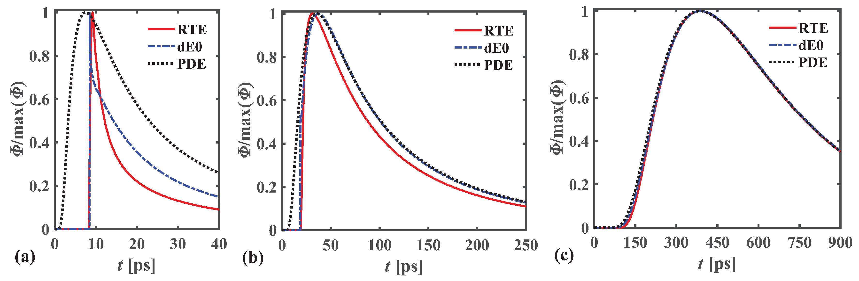
$t_{peak}^{ball}$ represents the arriving time of photons to the detector position without scattering, and $t_{peak}^{diff}$ the peak time for the diffusive photons calculated from the PDE (Equation (12)), respectively. Figure 4 show examples of the temporal profiles of $\mathsf{\Phi }(r,t)$ at the three characteristic length regimes. Here, we used the analytical solutions with the optical properties for the parameter set A as listed in Table 1 corresponding to the highly forward scattering of photons. While the RTE can appropriately treat the highly forward scattering, the dE0 and PDE approximate the highly forward scattering to the isotropic scattering. As shown in Figure 4a corresponding to the ballistic regime, the $\mathsf{\Phi }$-profiles using the RTE and dE0 are sharp, although both profiles are different from each other. The sharp profiles mean that photons are little scattered and travel almost straight. The peak times $t_{peak}$ for the RTE and dE0 are almost the same as the arriving time $t_{peak}^{ball}$, whose value is approximately 8.4 ps. Meanwhile, the broad profile of $\mathsf{\Phi }$ using the PDE is observed, indicating the unphysical multiple scattering of photons. In addition, the $t_{peak}$-value for the PDE is shorter than the $t_{peak}^{ball}$-value, meaning the violation of the causality in the PDE. As shown in Figure 4b corresponding to the scattering regime, the profiles using all the equations have smooth peaks. These peaks are formed by scattering of photons, so that these peak times are longer than $t_{peak}^{ball}$, in other words, the paths of photons are longer than the SD distance. In Figure 4b, the peak times for the dE0 and PDE are different from that for the RTE, indicating that the forward scattering of photons is not approximated to the isotropic scattering in this regime. As shown in Figure 4c corresponding to the diffusive regime, all the profiles are almost the same to each other, meaning the photon scattering becomes diffusive and the isotropic scattering approximation holds.

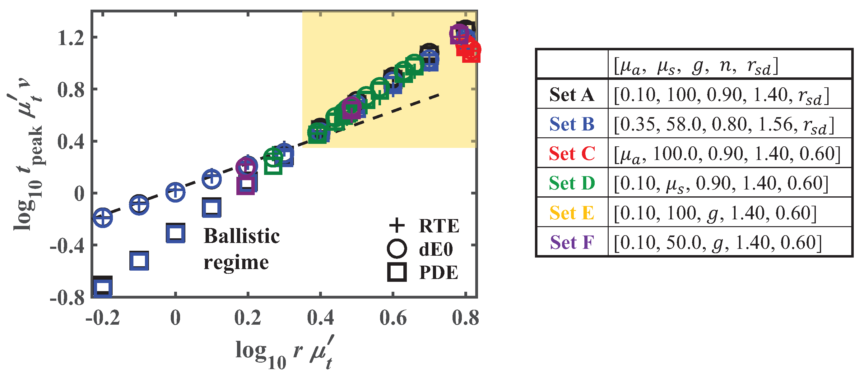
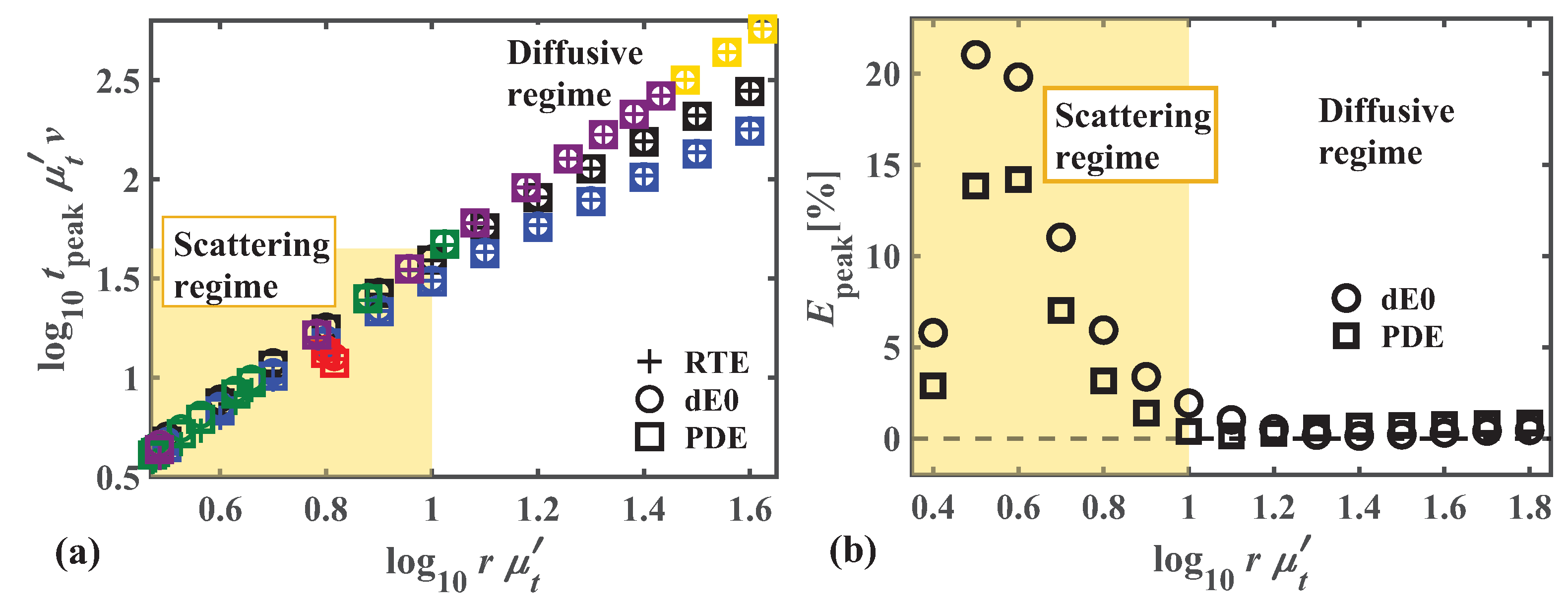
We evaluated crossover lengths and times from the ballistic to scattering regimes, and from the scattering to diffusive regimes, respectively, by investigating $t_{peak}$ for the RTE, dE0, and PDE. Then, we normalized the SD distance r by ${\mu }_t^{\prime }$ and the peak time $t_{peak}$ by ${\mu }_t^{\prime }v$, respectively, with the reduced transport coefficient of ${\mu }_t^{\prime }={\mu }_s(1-g)+{\mu }_a$. The inverses of ${\mu }_t^{\prime }$ and ${\mu }_t^{\prime }v$ correspond to the characteristic length and time for the dE0 and PDE where photons experience single scattering and absorbing processes. The normalizations allow us to investigate general features of photon transport in various kinds of random media. Figure 5 shows the results of the normalized peak times as a function of the normalized SD distances for the parameter sets A to F listed in Table 1 in a regime of short length and time scales. Here, the colors of the figures correspond to the parameter sets, e.g., the black colored pluses, circles, and squares correspond to the results for the parameter set A. In the regime of ${log}_{10}r{\mu }_t^{\prime }\lesssim 0.35$ and ${log}_{10}{t}_{peak}{\mu }_t^{\prime }v\lesssim 0.35$, the $t_{peak}$-results for the RTE and dE0 are linearly related to r, while the results for the PDE are not. This result suggests that the regime of the length and time scales correspond to the ballistic regime; and the crossover length and time from the ballistic to scattering regimes are evaluated as approximately ${10}^{0.35}/{\mu }_t^{\prime }\sim 2.2/{\mu }_t^{\prime }$ and ${10}^{0.35}/{\mu }_t^{\prime }v\sim 2.2/{\mu }_t^{\prime }v$, respectively.

Figure 6a shows the $t_{peak}$-results in a regime of longer length and time scales than the ballistic regime. In the case of the same parameter set (the same colored figures), the $t_{peak}$-results for the dE0 and PDE deviate from those for the RTE in the regime of $0.35\lesssim {log}_{10}r{\mu }_t^{\prime }\lesssim 1.0$ and $0.35\lesssim {log}_{10}{t}_{peak}{\mu }_t^{\prime }v\lesssim 1.6$, while the results for all the equations are almost the same to each other in the regime of $1.0\lesssim {log}_{10}r{\mu }_t^{\prime }$ and $1.6\lesssim {log}_{10}{t}_{peak}{\mu }_t^{\prime }v$. For the further investigation of $t_{peak}$, we evaluated the relative errors $E_{peak}$ of $t_{peak}$ against the RTE, defined by

$$E_{peak}=\left|\frac{t_{peak}-t_{peak,RTE}}{t_{peak,RTE}}\right|\times 100,t_{peak}=\{t_{peak,dE0},t_{peak,PDE}\}.$$

(16)

Although we calculated $E_{peak}$ for all the parameter sets, we showed the results only for the parameter set A in Figure 6b because the results for the other parameter sets behave similarly to the results for the parameter set A. As shown in Figure 6b, the $E_{peak}$-values for the dE0 and PDE are larger than 2% in the regime of $0.35\lesssim {log}_{10}r{\mu }_t^{\prime }\lesssim 1.0$. Here the $E_{peak}$-value of 2% is considered as a thresh to determine whether the dE0 and PDE are valid or not. The large $E_{peak}$-values indicate the strong influence of modeling the forward scattering on the $\mathsf{\Phi }$-results in this regime. Meanwhile, the $E_{peak}$-values for the dE0 and PDE are less than 2% in the regime of $1.0\lesssim {log}_{10}r{\mu }_t^{\prime }$, meaning the isotropic scattering approximation holds. From these results, the crossover length and time from the scattering to diffusive regimes are evaluated as approximately ${10}^1/{\mu }_t^{\prime }=10/{\mu }_t^{\prime }$ and ${10}^{1.6}/{\mu }_t^{\prime }v\sim 40/{\mu }_t^{\prime }v$, respectively. The crossover length from the scattering to diffusive regimes has been extensively discussed so far, and our evaluation is consistent with the previous studies such as a comparative study of the measurement data and the PDE-results for 3D slab media [10], and a comparative study of the numerical results using the RTE and PDE for 2D square media [9]. This consistency implies that boundary conditions less influence the crossover length because the previous studies consider the finite media, while this study the infinite media. Meanwhile, the crossover time from the scattering to diffusive regimes is longer than that evaluated by the previous study [9], which is approximately $20/{\mu }_t^{\prime }v$. The difference probably comes from the dimension of the medium and boundary effects; the previous study considers 2D finite media, while this study the 3D infinite media.

The dependence of the $t_{peak}$-results on the parameter sets is observed in the diffusive regime as shown in Figure 6a. This is because that in the diffusive regime, the normalizations of $t_{peak}$ by ${\mu }_{a}v$ and of $r^2$ by ${\mu }_a/D$ are appropriate, which are suggested from the form of $t_{peak}^{diff}$ (Equation (15)). As a preliminary study, we confirmed that when the above normalizations are employed, the $t_{peak}$-results for all the parameter sets are collapsed on a single curve in the diffusive regime. However, for the evaluation of the crossover length and time from the scattering to diffusive regimes, the above normalizations are not appropriate because the length regime, where the $E_{peak}$-values are larger than 2%, depends on the parameter sets, so that we can not evaluate the crossover length uniquely for all the parameter sets.

3.2. Length and Time Scales for the dEM to Be Valid in the Scattering Regime

In this subsection, we investigated the temporal profiles of the fluence rate $\mathsf{\Phi }(r,t)$ and their peak times $t_{peak}$ for the RTE and dEM in the scattering regime for the purpose of evaluations of the length and time scales for the dEM to be valid. As mentioned in Section 2.1.3, for the dEM, the scattering length scale is modified to the inverse of ${\mu }_s^M$ from the inverse of ${\mu }_s$, and the highly forward scattering of photons described by $p_{HG}$ is approximated to $p_{\delta 2}^M$. These modifications influence the results of $\mathsf{\Phi }(\mathit{r},t)$.

Firstly, we calculated $\mathsf{\Phi }(r,t)$ and $t_{peak}$ for the dEM at different g-values of 0.3, 0.6, 0.9, and 0.95 in the scattering length regime, and investigated the dependence of the results of $\mathsf{\Phi }(r,t)$ and $t_{peak}$ on the expansion order M and on the g-value. The optical properties and SD distance are set as ${\mu }_a=0.10$ ${\mathrm{cm}}^{-1}$, ${\mu }_s^{\prime }={\mu }_s(1-g)=10.0$ ${\mathrm{cm}}^{-1}$, $n=1.40$, and $r=0.32$ cm, where the normalized SD distance is constant as $\sim {10}^{0.5}/{\mu }_t^{\prime }$. Figure 7a shows the temporal profiles of $\mathsf{\Phi }(r,t)$ for the RTE and dEM with $M=0$, 1, and 2 (dE0, dE1, and dE2) at $g=0.9$, corresponding to the highly forward scattering. While the $\mathsf{\Phi }$-profile for the dE0 largely deviates from that for the RTE, the profiles for the dE1 and dE2 are similar to that for the RTE. Moreover, we investigated the relative error $E_{peak}^M$ of the peak time for the dEM:

$$E_{peak}^M=\left|\frac{t_{peak,dEM}-t_{peak,RTE}}{t_{peak,RTE}}\right|\times 100,$$

(17)

where $t_{peak,dEM}$ represents the peak time of $\mathsf{\Phi }(r,t)$ for the dEM. As shown in Figure 7b, the $E_{peak}^M$-values are quite small when the expansion order M is larger than 2 at all the g-values. This result means that the dEM with $M>2$ can provide the same accuracy as the RTE, almost independently of the g-values. Meanwhile, as shown in Figure 2, the g-dependences are observed in the ratios of ${\mu }_s^M/{\mu }_s$ and the errors of the phase function $E_{phase}^M$. These results suggest that for the accurate calculations of $\mathsf{\Phi }(r,t)$ using the RTE and dEM, it is sufficient to satisfy a few orders moment conditions of the phase function and the exact agreement of the profiles of the phase functions is not required. It is noted that the analytical results of the small $E_{peak}^M$-values with $M>2$ are quite different from the numerical calculations. The numerical results for the dEM are usually accurate within a finite range of M, and when the M-value is larger than the maximum value of the finite range, the numerical results for the dEM largely deviate from those for the RTE because of the numerical errors induced by angular discretization.

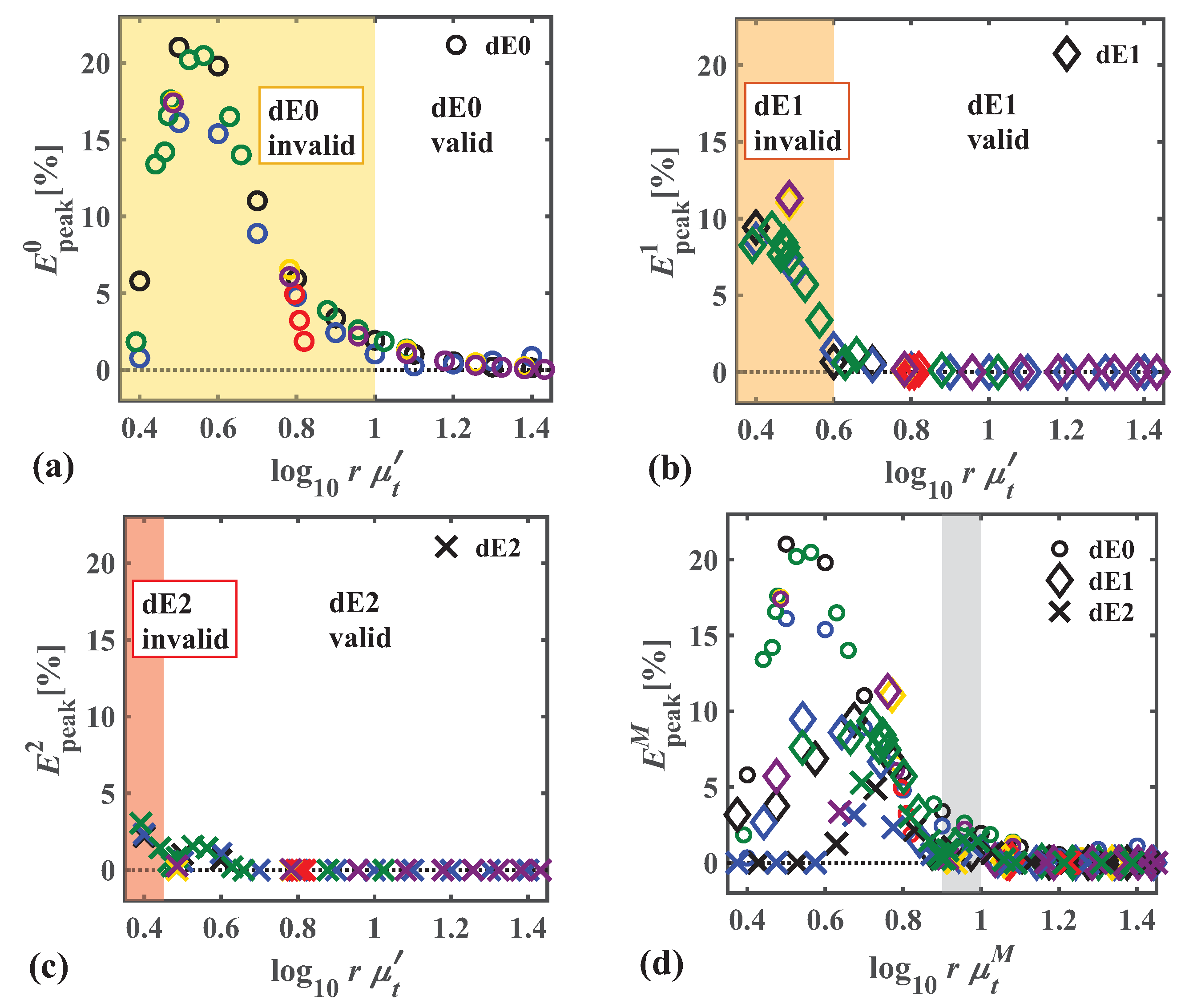
On the above discussion, we investigated $E_{peak}^M$ for the dEM at the constant normalized SD distance. Next, we investigated $E_{peak}^M$ for the dE0, dE1, and dE2 at the normalized SD distances varied from the scattering to diffusive regimes. Then, we evaluated the crossover lengths for the dE0, dE1, and dE2; in a regime of a smaller length scale than the crossover length, the $E_{peak}^M$-values are larger than 2%, corresponding to the invalidity of the dEM, while in a regime of a longer length scale, the errors are smaller than 2%, corresponding to the validity of the dEM. Figure 8a–c show the $E_{peak}^M$-values as a function of the normalized SD distances at the parameter sets A to F listed in Table 1. While the max value of $E_{peak}^M$ for the dE0 is over 20%, the max values for the dE1 and dE2 are around 10% and 4%, respectively. The length regime for the dE2 where the $E_{peak}^M$-values are larger than 2% is shorter than those for the dE0 and dE1. From the results in the figures (a), (b), and (c), we evaluated the crossover lengths for the dE0, dE1, and dE2 as approximately ${10}^1/{\mu }_t^{\prime }=10/{\mu }_t^{\prime }$, ${10}^{0.6}/{\mu }_t^{\prime }\sim 4.0/{\mu }_t^{\prime }$, and ${10}^{0.45}/{\mu }_t^{\prime }\sim 2.8/{\mu }_t^{\prime }$, respectively. These results mean that the scattering regime is classified into the three kinds of regimes by the two kinds of the crossover lengths for the dE1 and dE2. Here, we evaluated the crossover lengths for the dE0, dE1, and dE2 as a function of ${\mu }_t^{\prime }$ for the purpose of the classifications of the scattering regime. As an alternative, we can consider the normalization of the SD distances by ${\mu }_t^M={\mu }_s^M+{\mu }_a$ because for the dEM, the inverse of ${\mu }_t^M$ is the characteristic length of single scattering and absorption processes. Figure 8d shows $E_{peak}^M$ for the dE0, dE1, and dE2 as a function of the SD distances by ${\mu }_t^M$. The crossover lengths for the dEM with $M=0$, 1, and 2 are within the regime of $0.9\lesssim {log}_{10}r{\mu }_t^M\lesssim 1.0$, less dependently on the expansion order M. It is noted that the crossover length from the scattering and diffusive regimes depends on the expansion order M in the normalization by ${\mu }_t^M$, so that we cannot evaluate the regime for the dEM to be valid uniquely in the normalization. The rough evaluation of the crossover length for the dEM as $10/{\mu }_t^M$ means that after ten times scattering and absorption processes for the dEM, the M-th order dEA holds.

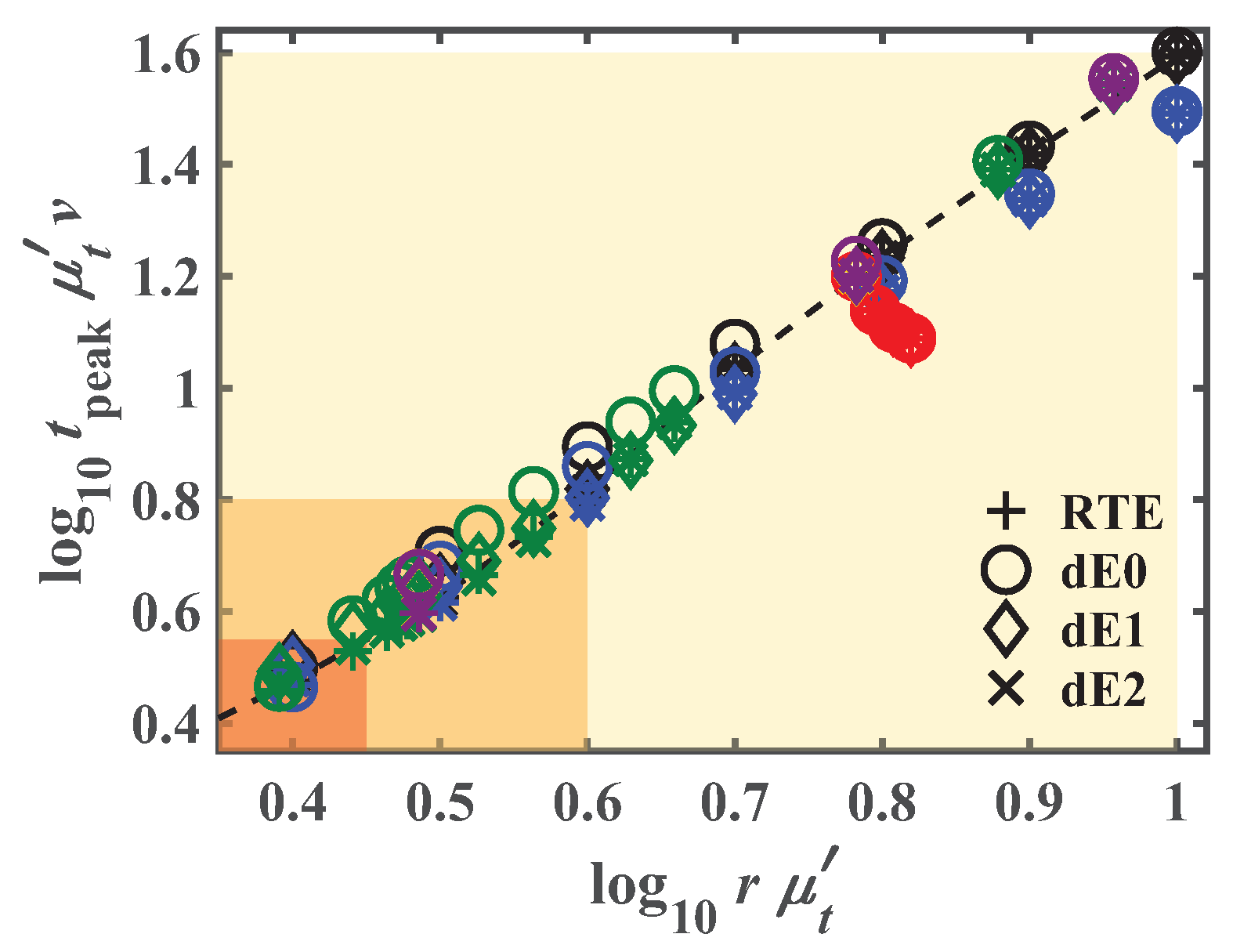
Figure 9 shows the normalized peak times for the RTE, dE0, dE1, and dE2 as a function of the normalized SD distances by ${\mu }_t^{\prime }$. From the figure and the results for the crossover lengths based on ${\mu }_t^{\prime }$, we evaluated the crossover times for the dE0, dE1, and dE2 as approximately ${10}^{1.6}/{\mu }_t^{\prime }v\sim 40/{\mu }_t^{\prime }v$, ${10}^{0.8}/{\mu }_t^{\prime }v\sim 6.3/{\mu }_t^{\prime }v$, and ${10}^{0.55}/{\mu }_t^{\prime }v\sim 3.5/{\mu }_t^{\prime }v$, respectively. Here, the evaluations of the crossover times are based on the $t_{peak}$-results for the RTE (dashed line in Figure 9 at the parameter set A) because the RTE is the most accurate photon transport model.

3.3. Influence of the Boundary Conditions on the Crossover Lengths and Times

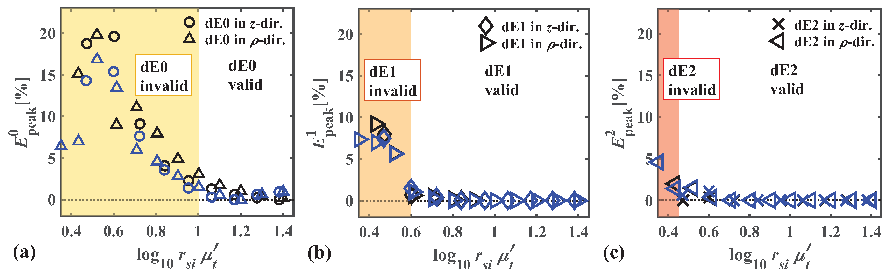
In this subsection, we investigated the boundary effects on the fluence rate $\mathsf{\Phi }(\mathit{r},t)$ and on the crossover lengths and times for the dEM with $M=0$, 1, and 2 by comparing the analytical solutions for the semi-infinite media with those for the infinite media. We considered the parameter sets A and B listed in Table 1, and varied the SD distances, denoted by $r_{si}=|\mathit{r}-{\mathit{r}}^{+}|$, in the two directions: the z-direction with $\mathit{r}=(0,0,z)$ and $\rho$-direction with $\mathit{r}=(\mathbf{\rho },0)$ as shown in Figure 3b. For the case of the detector position in the z-direction, as the z-value increases, the detector position becomes far from the boundary, so that the boundary effects probably become weak. Meanwhile, for the case of the detector position in the $\rho$-direction, a distance between the detector and the boundary is unchanged, so that the boundary effects are also unchanged. Figure 10a–c show the relative errors $E_{peak}^M$ for the dE0, dE1, and dE2 in the semi-infinite media as a function of the normalized SD distance by ${\mu }_t^{\prime }$. The crossover lengths for the dEM in the semi-infinite media are almost the same as those in the infinite media, meaning less influences of the boundary conditions on the crossover lengths.

Figure 11 shows the normalized peak times for the RTE in the infinite and semi-infinite media as a function of the SD distances $r_{sd}$ for the parameter sets A and B. Here, the SD distances $r_{sd}$ are given by r in infinite media, and by $r_{si}$ in semi-infinite media, respectively. The $t_{peak}$-results in the infinite media and semi-infinite media at the z-direction behave similarly to each other on the whole regime. Meanwhile, the $t_{peak}$-results in the semi-infinite media at the $\rho$-direction (dotted line in Figure 11 for the results at the parameter set A) are smaller than those in the other two cases (dashed line) especially on the regime of the longer length scale than approximately ${10}^{0.6}/{\mu }_t^{\prime }\sim 4.0/{\mu }_t^{\prime }$, which is almost the same as the crossover length for the dE1. These results suggest that the boundary conditions influence the crossover time for the dE0, while they have less influence the times for the dE1 and dE2.

4. Conclusions

We investigated the temporal profiles of the fluence rate $\mathsf{\Phi }(\mathit{r},t)$ and their peak times $t_{peak}$ for various kinds of random media at different SD distances by analytical solutions of the RTE, dE0, and PDE for 3D infinite homogeneous media. We evaluated the crossover lengths and times from the ballistic to scattering (few-scattering-event) regimes, and from the scattering to diffusive regimes as approximately $2.2/{\mu }_t^{\prime }$ and $2.2/{\mu }_t^{\prime }v$; $10/{\mu }_t^{\prime }$ and $40/{\mu }_t^{\prime }v$, respectively.

Next, we investigated $\mathsf{\Phi }(\mathit{r},t)$ and $t_{peak}$ for the dEM mainly in the scattering regime. We found that the results for the dE0 are quite similar to the results for the PDE because the dE0 and PDE approximate the forward scattering of photons as the isotropic scattering. We also found that at the expansion order of M larger than 2, the results for the dEM are almost the same as those for the RTE in the scattering and diffusive regimes, meaning the validity of the dEM with $M>2$ in the regimes. We evaluated the crossover lengths and times for the dE1 and dE2 as approximately $4.0/{\mu }_t^{\prime }$ and $6.3/{\mu }_t^{\prime }v$; $2.8/{\mu }_t^{\prime }$ and $3.5/{\mu }_t^{\prime }v$, respectively.

Finally, we investigated the boundary effects on the characteristic length and time scales of photon transport by comparing the results for the infinite media with those for the semi-infinite media. We found that the boundary conditions less influence on the crossover lengths for the dE0, dE1, and dE2, while the boundary conditions reduce the $t_{peak}$-values from those for bulk in the regime of the longer length scale than $4.0/{\mu }_t^{\prime }$, which is the same as the crossover length for the dE1. Hence, the crossover times for the dE1 and dE2 are less influenced by the boundary conditions. Our findings are useful for constructions of accurate and efficient photon transport models especially in the scattering regime.

References

- Gibson, A.P.; Hebden, J.C.; Arridge, S.R. Recent advances in diffuse optical imaging. Phys. Med. Biol. 2005, 50, R1–R43. [Google Scholar] [CrossRef] [PubMed]
- Okawa, S.; Hoshi, Y.; Yamada, Y. Improvement of image quality of time-domain diffuse optical tomography with lp sparsity regularization. Biomed. Opt. Express 2011, 2, 3334–3348. [Google Scholar] [CrossRef] [PubMed] [Green Version]
- Yamada, Y.; Okawa, S. Diffuse Optical Tomography: Present Status and Its Future. Opt. Rev. 2014, 21, 185–205. [Google Scholar] [CrossRef]
- Yamada, Y.; Suzuki, H.; Yamashita, Y. Time-Domain Near-Infrared Spectroscopy and Imaging: A Review. Appl. Sci. 2019, 9, 1127. [Google Scholar] [CrossRef] [Green Version]
- Ntziachristos, V. Going deeper than microscopy: The optical imaging frontier in biology. Nat. Methods 2010, 7, 603–614. [Google Scholar] [CrossRef] [PubMed]
- Bizheva, K.K.; Siegel, A.M.; Boas, D.A. Path-length-resolved dynamic light scattering in highly scattering random media: The transition to diffusing wave spectroscopy. Phys. Rev. E 1998, 58, 7664–7667. [Google Scholar] [CrossRef] [Green Version]
- Guerin, W.; Chong, Y.D.; Baudouin, Q.; Liertzer, M.; Rotter, S.; Kaiser, R. Diffusive to quasi-ballistic random laser: Incoherent and coherent models. J. Opt. Soc. Am. B 2016, 33, 1888–1896. [Google Scholar] [CrossRef] [Green Version]
- Tarvainen, T.; Vauhkonen, M.; Kolehmainen, V.; Kaipio, J. A hybrid radiative transfer – diffusion model for optical tomography. Appl. Opt. 2005, 44, 876–886. [Google Scholar] [CrossRef]
- Fujii, H.; Okawa, S.; Yamada, Y.; Hoshi, Y. Hybrid model of light propagation in random media based on the time-dependent radiative transfer and diffusion equations. J. Quant. Spectrosc. Radiat. Transfer 2014, 147, 145–154. [Google Scholar] [CrossRef] [Green Version]
- Yoo, K.M.; Liu, F.; Alfano, R.R. When does the diffusion approximation fail to describe photon transport in random media? Phys. Rev. Lett. 1990, 64, 2647–2650. [Google Scholar] [CrossRef]
- Hielscher, A.H.; Alcouffe, R.E.; Barbour, R.L. Comparison of finite-difference transport and diffusion calculations for photon migration in homogeneous and heterogeneous tissues. Phys. Med. Biol. 1998, 43, 1285–1302. [Google Scholar] [CrossRef] [PubMed]
- Venugopalan, V.; You, J.S.; Tromberg, B.J. Radiative transport in the diffusion approximation: An extension for highly absorbing media and small source-detector separations. Phys. Rev. E 1998, 58, 2395–2407. [Google Scholar] [CrossRef] [Green Version]
- Machida, M.; Panasyuk, G.Y.; Schotland, J.C.; Markel, V.A. The Green’s function for the radiative transport equation in the slab geometry. J. Phys. A Math. Theor. 2010, 43, 065402. [Google Scholar] [CrossRef]
- Fujii, H.; Hoshi, Y.; Okawa, S.; Kosuge, T.; Kohno, S. Numerical modeling of photon propagation in biological tissue based on the radiative transfer equation. In Proceedings of the 4th International Symposium on Slow Dynamics in Complex Systems, Sendai, Japan, 2–7 December 2013; Volume 1518, pp. 579–585. [Google Scholar]
- Fujii, H.; Okawa, S.; Yamada, Y.; Hoshi, Y.; Watanabe, M. A coupling model of the radiative transport equation for calculating photon migration in biological tissue. In Proceedings of the SPIE for Biophotonics Japan, Tokyo, Japan, 27–28 October 2015; Volume 9792, pp. 1–5. [Google Scholar]
- Joseph, J.H.; Wiscombe, W.J.; Weinman, J.A. The delta-Eddington approximation for radioactive flux transfer. J. Atmos. Sci. 1976, 33, 2452–2459. [Google Scholar] [CrossRef]
- Welch, A.; van Gemert, M. Optical-Thermal Response of Laser-Irradiated Tissue; Plenum Press: London, UK, 1995. [Google Scholar]
- Klose, A.D.; Hielscher, A.H. Modeling Photon Propagation In Anisotropically Scattering Media with the Equation Of Radiative Transfer. Proc. SPIE 2003, 4955, 624–633. [Google Scholar]
- Cong, W.; Shen, H.; Cong, A.; Wang, Y.; Wang, G. Modeling photon propagation in biological tissues using a generalized Delta-Eddington phase function. Phys. Rev. E 2007, 76, 051913. [Google Scholar] [CrossRef] [Green Version]
- Boulet, P.; Collin, A.; Consalvi, J.L. On the finite volume method and the discrete ordinates method regarding radiative heat transfer in acute forward anisotropic scattering media. J. Quant. Spectrosc. Radiat. Transfer 2007, 104, 460–473. [Google Scholar] [CrossRef]
- Klose, A.D.; Hielscher, A.H. Optical tomography with the equation of radiative transfer. Int. J. Numer. Methods Heat Fluid Flow 2008, 18, 443–464. [Google Scholar] [CrossRef]
- Jia, J.; Kim, H.K.; Hielscher, A.H. Fast linear solver for radiative transport equation with multiple right hand sides in diffuse optical tomography. J. Quant. Spectrosc. Radiat. Transfer 2015, 167, 10–22. [Google Scholar] [CrossRef] [Green Version]
- Kamran, F.; Abildgaard, O.H.A.; Subash, A.A.; Andersen, P.E.; Andersson-engels, S.; Khoptyar, D. Computationally effective solution of the inverse problem in time-of-flight spectroscopy. Opt. Express 2015, 23, 6937–6945. [Google Scholar] [CrossRef] [Green Version]
- Qin, J.; Lu, R. Measurement of the optical properties of fruits and vegetables using spatially resolved hyperspectral diffuse reflectance imaging technique. Postharvest Biol. Technol. 2008, 49, 355–365. [Google Scholar] [CrossRef]
- Chandrasekhar, S. Radiative Transfer; Dover: New York, NY, USA, 1960. [Google Scholar]
- Henyey, L.G.; Greenstein, L.J. Diffuse radiation in the galaxy. J. Astrophys. 1941, 93, 70–83. [Google Scholar] [CrossRef]
- Cheong, W.F.; Prahl, S.A.; Welch, A.J. A review of the optical properties of biological tissue. IEEE J. Quantum Electron 1990, 26, 2166–2185. [Google Scholar] [CrossRef] [Green Version]
- Germer, C.T.; Roggan, A.; Ritz, J.P.; Isbert, C.; Albrecht, D.; Müller, G.; Buhr, H.J. Optical properties of native and coagulated human liver tissue and liver metastases in the near infrared range. Lasers Surg. Med. 1998, 23, 194–203. [Google Scholar] [CrossRef]
- Dehaes, M.; Gagnon, L.; Vignaud, A.; Valabr, R.; Grebe, R.; Wallois, F.; Benali, H. Quantitative investigation of the effect of the extra-cerebral vasculature in diffuse optical imaging: A simulation study. Biomed. Opt. Express 2011, 2, 680–695. [Google Scholar] [CrossRef] [Green Version]
- Furutsu, K.; Yamada, Y. Diffusion approximation for a dissipative random medium and the applications. Phys. Rev. E 1994, 50, 3634–3640. [Google Scholar] [CrossRef]
- Liemert, A.; Kienle, A. Infinite space Green’s function of the time-dependent radiative transfer equation. Biomed. Opt. Express 2012, 3, 543. [Google Scholar] [CrossRef] [Green Version]
- Fujii, H.; Yamada, Y.; Chiba, G.; Hoshi, Y.; Kobayashi, K.; Watanabe, M. Accurate and efficient computation of the 3D radiative transfer equation in highly forward-peaked scattering media using a renormalization approach. J. Comput. Phys. 2018, 374, 591–604. [Google Scholar] [CrossRef]
- Paasschens, J.C.J. Solution of the time-dependent Boltzmann equation. Phys. Rev. E 1997, 56, 1135–1141. [Google Scholar] [CrossRef]
- Martelli, F.; Sassaroli, A.; Pifferi, A.; Torricelli, A.; Spinelli, L.; Zaccanti, G. Heuristic Green’s function of the time dependent radiative transfer equation for a semi-infinite medium. Opt. Express 2007, 15, 18168–18175. [Google Scholar] [CrossRef]
- Chandrasekhar, S. Stochastic Problems in Physics and Astronomy. Rev. Mod. Phys. 1943, 15, 1–88. [Google Scholar] [CrossRef]
- Egan, W.G.; Hilgeman, T.W. Optical Properties of Inhomogeneous Materials; Academic: New York, NY, USA, 1979. [Google Scholar]
- Patterson, M.S.; Chance, B.; Wilson, B.C. Time resolved reflectance and transmittance for the non- invasive measurement of tissue optical properties. Appl. Opt. 1989, 28, 2331–2336. [Google Scholar] [CrossRef] [PubMed]
- Simon, E.; Foschum, F.; Kienle, A. Hybrid Green’s function of the time- dependent radiative transfer equation for anisotropically scattering semi-infinite media scattering semi-infinite media. J. Biomed. Opt. 2013, 18, 015001. [Google Scholar] [CrossRef] [PubMed]
- Klose, A.D.; Netz, U.; Beuthan, J.; Hielscher, A.H. Optical tomography using the time-independent equation of radiative transfer - Part 1: Forward model. J. Quant. Spectrosc. Radiat. Transfer 2002, 72, 691–713. [Google Scholar] [CrossRef]
- Fujii, H.; Chiba, G.; Yamada, Y.; Hoshi, Y.; Kobayashi, K. Numerical treatment of highly forward scattering on radiative transfer using the delta-M approximation and Galerkin quadrature method. In Proceedings of the 9th International Symposium on Radiative Transfer, RAD-19, Athens, Greece, 3–7 June 2019; pp. 261–268. [Google Scholar]
Figure 1.
Henyey-Greenstein phase function as a function of for isotropic scattering (), moderately forward scattering (), and highly forward scattering ( and 0.95), in a logarithmic scale.
Figure 2.
(a) Ratios and (b) relative errors of the phase functions between the HG function (Equation (2)) and the M-th order dEA (Equation (5)) at different g-values of 0.3, 0.6, 0.9 and 0.95. The error is defined by Equation (8).
Figure 3.
Source and detector positions in 3D (a) infinite and (b) semi-infinite homogeneous media.
Figure 4.
Analytical solutions of the RTE (Equation (10)), dE0 (Equation (11) with ), and PDE (Equation (12)) at the three characteristic length regimes of photon transport: (a) ballistic regime at the SD distance of cm (), (b) scattering regime at cm (), and (c) diffusive regime at cm (). The optical properties at the parameter set A are used, which are listed in Table 1.
Figure 5.
Normalized peak times by as a function of the normalized SD distances r by for the RTE, dE0, and PDE in the ballistic and scattering regimes. represents the reduced transport coefficient and v the speed of light in a medium, respectively. Colors of the figures correspond to the results for the parameter sets A to F listed in Table 1 or in the legend at the right-side of the figure. The dashed line represents the linear relation between and r. The yellow colored area corresponds to the scattering regime.
Figure 6.
(a) Normalized peak times and (b) relative errors (Equation (16)) for the dE0 and PDE as a function of the normalized SD distances in the scattering and diffusive regimes. The other details are the same as Figure 5.
Figure 7.
(a) Temporal profiles of using the RTE, dE0, dE1, and dE2 at . (b) Relative errors of the peak time of (Equation (17) as a function of the expansion order M at different g-values of 0.3, 0.6, 0.9, and 0.95. The optical properties and SD distance are set as , , , and cm.
Figure 8.
Relative errors (Equation (17)) for the (a) dE0, (b) dE1, and (c) dE2 as a function of the normalized SD distances by at the parameter sets A to F listed in Table 1. The yellow, orange, and red colored areas correspond to the length regimes where the dE0, dE1, and dE2 are invalid, respectively. (d) Normalization of the SD distances by . The gray colored areas correspond to the crossover length for the dEM. The other details are the same as Figure 6.
Figure 9.
Normalized peak times of for the RTE, dE0, dE1, and dE2 as a function of the normalized SD distances. The dashed line represents the connection line for the RTE-results at the parameter set A. The other details are the same as Figure 8a–c.
Figure 10.
Relative errors for the (a) dE0, (b) dE1, and (c) dE2 in the semi-infinite media (Figure 3b) as a function of the normalized SD distances at the parameter sets A and B listed in Table 1. The SD distances are varied in the z-direction with and in the -direction with . The other details are the same as Figure 8a–c.
Figure 11.
Normalized peak times for the RTE in infinite media, and semi-infinite media at the z- and -directions. The SD distances are given by r in infinite media and by in semi-infinite media, respectively. The dashed and dotted lines represent the connection lines for the results in infinite and semi-infinite media at the -direction, respectively, for the parameter set A. The other details are the same as Figure 10.