A Novel Optimization Algorithm Combing Gbest-Guided Artificial Bee Colony Algorithm with Variable Gradients

Abstract

The artificial bee colony (ABC) algorithm, which has been widely studied for years, is a stochastic algorithm for solving global optimization problems. Taking advantage of the information of a global best solution, the Gbest-guided artificial bee colony (GABC) algorithm goes further by modifying the solution search equation. However, the coefficient in its equation is based only on a numerical test and is not suitable for all problems. Therefore, we propose a novel algorithm named the Gbest-guided ABC algorithm with gradient information (GABCG) to make up for its weakness. Without coefficient factors, a new solution search equation based on variable gradients is established. Besides, the gradients are also applied to differentiate the priority of different variables and enhance the judgment of abandoned solutions. Extensive experiments are conducted on a set of benchmark functions with the GABCG algorithm. The results demonstrate that the GABCG algorithm is more effective than the traditional ABC algorithm and the GABC algorithm, especially in the latter stages of the evolution.

1. Introduction

As computer technology gains momentum, more and more researchers develop and apply optimization algorithms to solve optimization problems. These algorithms can be broadly divided into gradient-based and gradient-free (or stochastic) optimization algorithms. Gradient-based optimization algorithms search along the gradient direction. They are of high convergence rate and are particularly suitable for solving problems with large design space [1]. However, their optimization results are close to the extreme point near the point of the initial parameter, rather than the maximum point of the entire design space [2]. On the contrary, gradient-free optimization algorithms are robust and quite effective for solving multi-modal optimization problems [3]. Such algorithms can be easily integrated into different optimization designs, but they are computationally expensive, especially in cases of numerous design parameters [4]. Due to the feature of their random search, these stochastic algorithms tend to converge slowly [5], especially near the area of global optimum. Therefore, it is significant to improve the convergence of stochastic algorithms through some modifications.

First proposed by Karaboga [6], the artificial bee colony (ABC) algorithm is a gradient-free optimization algorithm that is widely used in multi-variable and multi-objective optimizations [7]. Karaboga’s further research [8,9] shows that the ABC algorithm outperforms other stochastic algorithms, such as the genetic algorithm (GA), particle swarm algorithm (PSO), and particle swarm inspired evolutionary algorithm (PS-EA). However, the ABC algorithm is good at exploration but poor at exploitation [10]. Integrating gradient-based searching method into evolution algorithms may improve exploitation [11,12,13,14]. In recent years, some novel algorithms based on gradient information have been brought forward to modify the ABC algorithm. For example, a hybrid algorithm called ABC-SQP was developed by Eslami [15]. It combines the artificial bee colony algorithm with sequential quadratic programming. Another algorithm, the gradient-based artificial bee colony algorithm (GdABC), was brought forward by Juan et al. [16] to improve the local search ability. Both ABC-SQP and GdABC use the global exploration capability of the ABC algorithm and the exploitation capability of gradient-based local search algorithm. However, in these hybrid algorithms, the search equation of the original program is not modified, and the procedures of the random searching algorithm and the gradient-based local search algorithm are independent of each other. Thus, the program parts of a gradient optimization still tend to fall into the local optimum.

Other researchers have improved the search strategy of ABC algorithm by modifying the search equation according to the information of best solutions [17,18,19,20]. For example, Zhu and Kwong [21] found that the global best solution could help improve exploitation. They proposed the Gbest-guided artificial bee colony search (GABC) algorithm. Due to the great advantage of the convergence property of GABC, many GABC-based algorithms have been developed [22,23,24,25,26,27]. For example, Guo et al. [22] incorporated the information of current iteration best solution into solution search equation and introduced global artificial bee colony search algorithm (GABCS). In the original GABC algorithm, the convergence performance is improved by adding a coefficient factor to the solution search equation. However, the selection of the coefficient factor is just based on testing. In the study of Zhu and Kwong, the best value of the coefficient factor they chose is not suitable for all problems. Therefore, the theoretical analysis and the conclusion of the GABC algorithm are inadequate. It is necessary to make up for this weakness.

We present an idea of establishing a new solution search equation leaving out the coefficient factor and introducing variable gradients. Since the gradient magnitude characterizes the effect of variable change on the solution, we also apply it to differentiate the priority of different variables and enhance the judgment of local optimum, simultaneously. In this paper, we present a novel optimization algorithm combing Gbest-guided artificial bee colony algorithm with variable gradients (the Gbest-guided ABC algorithm with gradient information—GABCG). This novel algorithm perfects the theory of the Gbest-guided artificial bee colony algorithm with a modified solution search equation. It accelerates the convergence rate of optimization algorithm by giving priority to variables with greater gradients and enhances the judgement on abandoned solutions with variable gradients to avoid premature abandonment of solutions. To validate the advantages of this new hybrid algorithm, a set of 10 well-known benchmark functions are considered to compare the performance of the traditional ABC, GABC, and GABCG algorithms. The experiment results demonstrate that the proposed algorithm is more effective than these two ABC-based algorithms, especially in the latter stages of the evolution. Finally, the characteristics of the improvement measures are discussed, and future research sites are indicated.

2. Overview of Artificial Bee Colony Algorithm

The ABC algorithm is a gradient-free algorithm inspired by the intelligent foraging behavior of a bee colony [22]. In this algorithm, there are three groups of artificial bees, including employed bees, onlookers and scouts [6]. Employed bees search food around the food source they have found. Onlooker bees, waiting at the dance area, take charge of selecting good food sources from those found by the employed bees. Scouts carry out random searches to expand the scope of exploration.

At the beginning of the algorithm process, the food solutions of employed bees are randomly initialed by Equation (1). These solutions and their nectar amounts are recorded as the first generation “food sources.” Then, the following steps are repeated until the best food source meets the colony’s requirements [28]:

• Every employed bee collects nectar at food sources according to Equation (2) [29];
• After food sources are selected in light of probability value (p_i in Equation (3), which is in direct proportion to nectar amount of food source), every artificial onlooker collects nectar at new food sources, which are generated according to Equation (2) [30];
• Employing greedy selection, the “food sources” in each iteration are updated by employed bees and onlookers;
• If the nectar amount of a food source has not increased more than “limit” (a control parameter) times, it will be abandoned, and a scout will search for a new food source according to Equation (1).

When the algorithm is terminated, the optimal food source solution and its nectar amount are outputted.

$$x_{ij}=x_{\min }+{\psi }_{ij}\left(x_{\max }-x_{\min }\right)$$

(1)

where i ∈ {1, 2,…, N}, j ∈ {1, 2,…, D}, N stands for the number of food sources and D represents the number of variable elements. x_ij represents jth element of ith source solution, and Ψ_ij is a random number in [0, 1].

$$v_{ij}=x_{ij}+{\varphi }_{ij}\left(x_{ij}-x_{kj}\right)$$

(2)

where Φ_ij is a random number in [−1, 1] and k is a randomly chosen index which is different from i.

$$p_i=\frac{F_i}{{\displaystyle \sum _{m=1}^N{F}_m}}$$

(3)

where F_i is the fitness value of the solution i evaluated by its employed bee, which is proportional to the nectar amount of the food source at position i.

3. The Gbest-Guided ABC Algorithm with Gradient Information

As illustrated in the Introduction, Zhu and Kwong [20] incorporated the information of global best solution into the solution equation and developed a better version of the ABC algorithm called the Gbest-guided ABC (GABC) algorithm. They modified the ABC algorithm by replacing Equation (2) with Equation (4), thus driving the new candidate solution toward the global best solution. Their study shows that the new solution search equation described by Equation (4) can increase the exploitation of the ABC algorithm, and the parameter C plays an important role in balancing the exploration and exploitation of the searching for the optimal solution. For most of the results of their cases, it can be observed that as the value of parameter C increases, the optimization results get better at first but then begin to deteriorate after a certain value. In their numerical experiments, GABC algorithm with C = 1.5 shows the best performance among the tested programs.

$$v_{ij}=x_{ij}+{\varphi }_{ij}\left(x_{ij}-x_{kj}\right)+C{\psi }_{ij}\left(y_j-x_{ij}\right)$$

(4)

where C is a non-negative constant parameter, Ψ_ij is a random number in [0, 1] and y_j is the jth element of the global best solution.

Actually, in Equation (4), y_j represents only the information of best solution found so far. There may be better solutions that have not been searched out by algorithm. In Figure 1, y_j with negative gradient value at jth element is represented by y_j′. Taking y_j′ as an example, if the value of C in Equation (4) is less than 1, the solutions generated by Equation (4) is closer to a solution on the left side of y_j′. In another case, if the value of C is much larger than 1, the solutions generated by Equation (4) is closer to a solution on the very right side of y_j′. But GABC algorithm prefers to search toward a small range (region A) on the right of y_j′ because there are better solutions in this area. Therefore, we suggest that 1.5 may be a relatively appropriate value of C for the cases that Zhu and Kwong studied.

Although the GABC algorithm can achieve good results when the parameter C is 1.5, it still has some inherent weakness. For example, in Figure 1, y_j″ has positive gradient value at the jth element and x_ij is less than y_j″. The solutions generated by Equation (4) with C = 1.5 is closer to a solution on the right side of y_j″, instead of better solutions on the left. Besides, because Zhu and Kwong only took a few discrete values for C, the optimal parameter value could not be accurately determined. In their calculations for the Rastrigin function, the program with C = 1 got better results than the program with C = 1.5. This means that C = 1.5 is not applicable to all optimization problems.

A more accurate estimation of the best solution may further improve the exploitation of algorithm. Since the GABC algorithm has these defects, we hope to propose new ideas on the solution search equation. As shown in Figure 1, better solutions may be on the left or right side of the current global best solution, which is related to the sign of the gradient. Therefore, we define the jth element of estimated best solution as follows: y_j − ζ_ij(y_j − z_j2)/2 (ζ_ij is a random number in [0, 1] and z_j2 is the rightmost solution of y_j) when the gradient value of y_j is negative, y_j − ζ_ij(y_j − z_j1)/2 (z_j1 is the leftmost solution of y_j) when the gradient value is positive and still y_j when the gradient value is zero. Taking advantage of the estimated best solution, the solution search equation used by employed bees and onlookers is converted into Equation (5). Therefore, the next generations of employed bees and onlookers look for better routes toward the estimated best solution of current generation. It should be noted that some methods can be employed to calculate the gradient of optimization problems, such as discrete estimation method (Equation (6) is used in this study) and the adjoint method [1, 4].

$$v_{ij}=x_{ij}+{\varphi }_{ij}\left(x_{ij}-x_{kj}\right)+{\psi }_{ij}\left(y_j-{\zeta }_{ij}\frac{y_j-z_j}{2}-x_{ij}\right)$$

(5)

$${\partial }_{y_j}f\approx \frac{1}{2}\left(\frac{f\left(y\right)-f\left(z_1\right)}{y_j-z_{j1}}+\frac{f\left(y\right)-f\left(z_2\right)}{y_j-z_{j2}}\right)$$

(6)

The gradient values of parameters contain two kinds of information: symbol and magnitude. The sign can be used to judge the direction of optimization, and the magnitude can determine the effect of variable changes on objective functions. With the help of the sign of the gradient, the above measure (Measure 1) ensures that the random search goes toward a solution that is better than the current global best solution. In addition, the gradient magnitude is applied in the following two other improvement measures:

Measure 2: In the ABC algorithm, an onlooker chooses a food source in light of probability value, which is determined by fitness. Similarly, in our newly proposed algorithm, when the global best solution is selected by an employed bee (or an onlooker), the variable element to be changed is determined by the probability value associated with the gradient. Detailed operations are as follows: Randomly selecting a variable element y_k and a random number q in [0, 1]. If pg_k in Equation (7) is greater than q, this element will be used for optimization; otherwise, re-random selection will be carried out until the judgment condition is met.

$$p{g}_k=\frac{\left|{\partial }_{y_k}F\right|}{{\displaystyle \sum _{m=1}^D\left|{\partial }_{y_m}F\right|}}$$

(7)

Measure 3: Since the gradient values of the solution near the vertex are relatively small, an abandoned solution can be judged not only by the control parameter (limitation of times) but also by the gradient magnitude. In our study, only when the fitness of a food source has not been improved more than limited times and all variable gradients of this source are less than 10 times maximum parameter gradient of the global best solution does the scout bee operate a random search.

Based on the above explanation of three improvement measures, the pseudo code of the GABCG algorithm is given as

Table 1. Pseudo code of the Gbest-guided ABC algorithm with gradient information (GABCG) algorithm.

//Control Parameters: CS: The colony size MC: Maximum cycle number in order to terminate the algorithm Limit: The control Parameter in order to abandoned the food source Bas: The counter for counting the number of being exploited Fit: The fitness of a food source Sen: The gradient of a variable element NormFit: The fitness probability of a food source NormSen: The gradient probability of a variable element for g from 1 to MC:   //Employed Bees Phase   for i from 1 to CS/2:   if GlobalMin = = Fit(i):    Randomly seletct a variable element j    if rand < NormSen(j):     Produce a new candidate solution by Equation (5)    else:     Reselect a variable element    end   else:    Produce a new candidate solution by Equation (5)   end   end   //Onlookers Phase   for i from 1 to CS/2:   if rand < NorFit(i):    if GlobalMin = = Fit(i):     Randomly seletct a variable element j     if rand < NormSen(j):      Produce a new candidate solution by Equation (5)     else:      Reselect a variable element end    else:    Produce a new candidate solution by Equation (5)    end   else:    Reselect a food source   end  end  Employ greed selection to food sources  //Scout Phase ind = max(Bas)   if Bas(ind) > Limit && all(abs(Sen(ind)) < 10*max(Sen(GlobalMin)):   Update the original solution using Equation (1) randomly   end  Remember the best solution obtained so far end

. Since the innermost loop body of the new algorithm has not changed, the complexity of each iteration does not greatly increase.

The whole search strategy adopted by the Gbest-guided ABC algorithm with gradient information (GABCG) is shown in Figure 2. In Measure 1, the sign of the gradient is applied to find a better solution than the current global best solution, so the exploitation is increased further in our proposed algorithm. In a standard ABC algorithm, the preference of a food source by an onlooker bee depends on the nectar amount of that food source. Inspired by this, the preference of a variable should depend on the gradient magnitude of that variable. Thus, through Measure 2, gradient values are used to evaluate the updating probability of variables, and the variables with a larger gradient have a greater chance of being selected to update. Besides, in the original algorithm, the scouts just control the exploration process through the predetermined number of trials “limit”. While, in our algorithm, the gradient magnitude is used as another evaluation criterion. Measure 3 strengthens the judgment of the abandoned solution by the gradient limit, so that it is effective for accurately determining whether the search is trapped in the local optimum.

4. Experiments

4.1. Benchmark Functions and Parameter Settings

In order to verify the validity of proposed GABCG algorithm, we conducted it on the maximum and minimum of functions. Some functions that are commonly used for optimization were chosen to confirm the effectiveness of the GABCG. f₁ − f₁₀ are shown in

Table 2. The 10 benchmark functions for experimental study.

f	Function	C	Initial Range	f(x*)
Rosenbrock	$f_1(\mathit{x})={\displaystyle \sum _{i=1}^{D-1}\left[100{\left(x_{i+1}-x_i{}^2\right)}^2+{\left(x_i-1\right)}^2\right]}$	UN	[−50,50]	$f(\overrightarrow{1})=0$
Sphere	$f_2(\mathit{x})={\displaystyle \sum _{i=1}^D{x}_i^2}$	US	[−100,100]	$f(\overrightarrow{0})=0$
Elliptic	$f_3(\mathit{x})={\displaystyle \sum _{i=1}^D{\left({10}^6\right)}^{\left(i-1\right)/\left(D-1\right)}{x}_i^2}$	UN	[−100,100]	$f(\overrightarrow{0})=0$
SumSquares	$f_4(\mathit{x})={\displaystyle \sum _{i=1}^{D}i{x}_i^2}$	US	[−10,10]	$f(\overrightarrow{0})=0$
Quartic	$f_5(\mathit{x})={\displaystyle \sum _{i=1}^{D}i{x}_i^4}$	US	[−1.28,1.28]	$f(\overrightarrow{0})=0$
Himmelblau	$f_6(\mathit{x})=\frac{1}{D}{\displaystyle \sum _{i=1}^D\left(x_i^4-16x_i^2+5x_i\right)}$	MS	[−5,5]	$\begin{array}{l}f(\overrightarrow{2.9035})=\\ 78.3323\end{array}$
Schaffer	$f_7(\mathit{x})=0.5+\frac{{\sin }^2\left(\sqrt{{\displaystyle {\sum }_{i=1}^D{x}_i{}^2}}\right)-0.5}{{\left(1+0.001\left({\displaystyle {\sum }_{i=1}^D{x}_i{}^2}\right)\right)}^2}$	MN	[−100,100]	$f(\overrightarrow{0})=0$
Rastrigin	$f_8(\mathit{x})={\displaystyle \sum _{i=1}^D(x_i^2-10\cos (2\pi x_i)+10)}$	MS	[−5.12,5.12]	$f(\overrightarrow{0})=0$
Griewank	$f_9(\mathit{x})=\frac{1}{4000}{\displaystyle \sum _{i=1}^D{x}_i^2}-{\displaystyle \prod _{i=1}^D\cos \left(\frac{x_i}{\sqrt{i}}\right)+1}$	MN	[−600,600]	$f(\overrightarrow{0})=0$
Ackley	$\begin{array}{l}{f}_{10}(\mathit{x})=20+e-20\exp \left(-0.2\sqrt{\frac{1}{D}{\displaystyle \sum _{i=1}^D{x}_i{}^2}}\right)\\ -\exp \left(\frac{1}{D}{\displaystyle \sum _{i=1}^D\cos \left(2\pi x_i\right)}\right)\end{array}$	MN	[−32.768,32.768]	$f(\overrightarrow{0})=0$

, which denote Rosenbrock, Sphere, Schaffer, Rastrigin, Griewank, Ackley, Elliptic, SumSquares, Quartic, and Himmelblau function, respectively [17]. Different letters indicate different characteristics. U stands for unimodal, and M stands for multimodal. S stands for separable, and N stands for non-separable. In this study, the Rosenbrock, Sphere, Elliptic, SumSquares, and Quartic functions (f₁ − f₅) with single-peak were used to verify the convergence accuracy and rate of the algorithm. Since many physical problems have multiple peaks, the optimization search may fall into a local optimum on the path towards the global optimum [5]. It is very important to test the optimization algorithm using multimodal functions. Therefore, the Himmelblau, Schaffer, Rastrigin, Griewank, and Ackley functions (f₆ − f₁₀) with multi-peak were used to verify the global optimization capability of the algorithm.

In our experiments, the main control parameters are set as follows: The colony size is 80 (the number of employed bees is 40, the number of onlookers is 40, and the number of scout bees is one). The maximum number of generations is 5000. The times “limit” of abandoning the food source is 50. The parameter C of the GABC algorithm is set as 1.5. Schaffer function and Rosenbrock function were tested with 10 and 30 variable elements, Himmelblau function was tested with 100 and 200 variable elements, and the other functions were tested with 30 and 60 variable elements. Each experiment was repeated 30 times by the ABC, GABC, and GABCG algorithms.

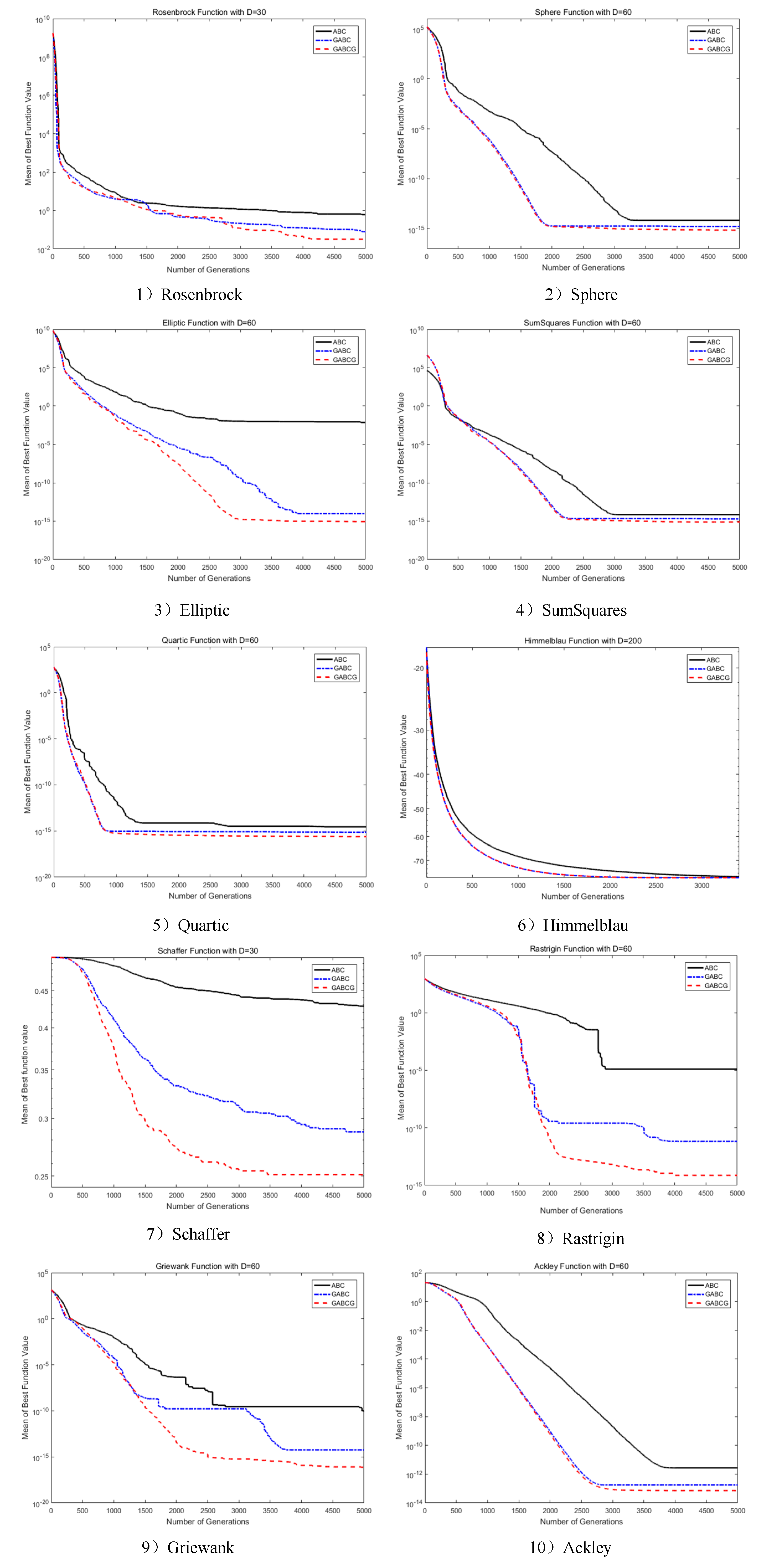
4.2. Performance Comparison between ABC, GABC, and GABCG

Comparing the proposed algorithm with the other two algorithms on 10 benchmark functions,

Table 3. Optimizations of benchmark functions by the artificial bee colony (ABC), Gbest-guided artificial bee colony (GABC), and GABCG algorithms.

Function	D	ABC		GABC		GABCG
		Mean	SD	Mean	SD	Mean	SD
Rosenbrock	10	4.25 × 10−1	2.19 × 10−1	3.40 × 10−2	1.73 × 10−2	1.47 × 10−2	1.46 × 10−2
	30	6.15 × 10−1	3.28 × 10−1	5.45 × 10−2	3.65 × 10−2	3.16 × 10−2	3.71 × 10−2
Sphere	30	7.62 × 10−16	1.47 × 10−16	4.33 × 10−16	6.79 × 10−16	2.39 × 10−18	3.36 × 10−17
	60	7.14 × 10−15	3.84 × 10−15	1.62 × 10−15	2.10 × 10−16	7.76 × 10−15	2.88 × 10−14
Elliptic	30	4.23 × 10−7	1.70 × 10−6	4.80 × 10−16	7.03 × 10−17	2.75 × 10−16	6.66 × 10−17
	60	7.22 × 10−3	7.63 × 10−3	9.89 × 10−15	1.57 × 10−14	1.21 × 10−15	7.63 × 10−16
SumSquares	30	7.43 × 10−15	1.06 × 10−16	4.37 × 10−16	4.87 × 10−17	2.17 × 10−16	3.62 × 10−17
	60	7.10 × 10−15	5.03 × 10−15	1.95 × 10−15	3.51 × 10−16	7.72 × 10−16	1.03 × 10−16
Quartic	30	2.78 × 10−16	6.52 × 10−17	1.07 × 10−16	3.37 × 10−17	5.55 × 10−17	1.71 × 10−17
	60	2.72 × 10−15	2.12 × 10−15	7.21 × 10−16	1.22 × 10−16	2.37 × 10−16	3.27 × 10−17
Himmelblau	100	−78.3323	1.28 × 10−11	−78.3323	1.04 × 10−13	−78.3323	6.01 × 10−14
	200	−78.3273	2.06 × 10−2	−78.3323	1.06 × 10−11	−78.3323	6.80 × 10−12
Schaffer	10	2.54 × 10−2	1.37 × 10−2	2.27 × 10−2	1.39 × 10−2	9.72 × 10−3	3.52 × 10−8
	30	4.24 × 10−1	2.59 × 10−2	2.87 × 10−1	4.19 × 10−2	2.51 × 10−1	3.61 × 10−2
Rastrigin	30	1.07 × 10−11	1.61 × 10−11	7.96 × 10−14	3.20 × 10−14	0	0
	60	1.27 × 10−5	4.53 × 10−5	6.68 × 10−12	1.04 × 10−11	1.14 × 10−14	3.47 × 10−14
Griewank	30	4.84 × 10−14	9.12 × 10−14	3.07 × 10−16	2.45 × 10−16	3.70 × 10−18	2.03 × 10−17
	60	8.62 × 10−11	4.55 × 10−10	2.20 × 10−14	5.17 × 10−14	6.66 × 10−17	1.29 × 10−16
Ackley	30	1.24 × 10−13	4.10 × 10−14	4.02 × 10−14	4.27 × 10−15	3.08 × 10−14	3.05 × 10−15
	60	2.72 × 10−12	1.50 × 10−12	1.79 × 10−13	3.22 × 10−14	7.15 × 10−14	5.34 × 10−15

Mean and SD donate the average and standard deviation of optimization results in 30 runs, and the best mean results are in bold.

shows the mean and standard deviations of each benchmark function results. The average convergence curves of representative cases are presented in Figure 3. It can be seen that the program using the GABCG algorithm gets better results on all 10 functions than the ABC algorithm and the GABC algorithm.

As seen from the results, the GABCG algorithm has great advantage of convergence property and applicability compared to the ABC and GABC algorithms. For the unimodal functions in Figure 3(1–5), the performances of the GABCG algorithm are both superior to the ABC algorithm and the GABC algorithm, which verifies the good convergence accuracy and rate of the GABCG algorithm. In Figure 3(6–10), it is more obvious to see the advantage of the GABCG algorithm in the accuracy of results for multimodal functions, which testifies the good global optimization capability of the GABCG algorithm. From these iterative curves, it can be seen that the GABCG algorithm shows better convergence performance than the GABC algorithm in the latter iterations.

Comparing the performance of the GABCG algorithm in unimodal functions and multimodal functions, it can be found that this algorithm is superior in solving most multi-peak problems. Especially on some complex problems, such as Rastrigin and Griewank functions, the results of both the ABC and GABC algorithms appear to be stagnant in the middle phases of evolution. However, the GABCG algorithm can keep finding better solutions during almost the entire search. This indicates that the GABCG algorithm successfully reduces unnecessary computation costs and determines the exact optimization paths by gradient acceleration.

4.3. Effects of the Colony Size on the Performance of GABCG

In order to analyze the effect of colony size on convergence speed and accuracy, the algorithm programs were run with different colony sizes. At first, we studied the three algorithms with 80, 160, and 240 colony sizes. Both the numbers of employed bees and onlooker are half of the colony size, and the number of scout bees is one. In this test, the programs were executed on five benchmark functions. Schaffer function and Rosenbrock function were tested with 30 variable elements, and the other functions were tested with 60 variable elements. Each experiment was repeated 30 times by the ABC, GABC, and GABCG algorithms.

The mean and standard deviations of optimization results are presented in

Table 4. Optimization results of the ABC, GABC, and GABCG algorithms with different colony sizes.

Function	CZ	ABC		GABC		GABCG
		Mean	SD	Mean	SD	Mean	SD
Rosenbrock	80	6.15 × 10−1	3.28 × 10−1	5.45 × 10−2	3.65 × 10−2	3.16 × 10−2	3.71 × 10−2
	160	2.33 × 10−1	9.72 × 10−2	4.98 × 10−2	3.29 × 10−2	2.20 × 10−2	2.56 × 10−2
	240	1.65 × 10−1	1.80 × 10−1	2.94 × 10−2	1.78 × 10−2	1.12 × 10−2	1.50 × 10−2
Elliptic	80	7.22 × 10−3	7.63 × 10−3	9.89 × 10−15	1.57 × 10−14	1.21 × 10−15	7.63 × 10−16
	160	1.04 × 10−4	6.44 × 10−5	1.83 × 10−15	3.44 × 10−16	6.50 × 10−16	8.46 × 10−17
	240	2.47 × 10−5	1.93 × 10−5	1.74 × 10−15	2.75 × 10−16	5.27 × 10−16	6.98 × 10−17
Schaffer	80	4.24 × 10−1	2.59 × 10−2	2.87 × 10−1	4.19 × 10−2	2.51 × 10−1	3.61 × 10−2
	160	3.95 × 10−1	1.81 × 10−2	2.41 × 10−1	3.12 × 10−2	2.30 × 10−1	5.60 × 10−2
	240	3.36 × 10−1	3.51 × 10−2	1.88 × 10−1	3.96 × 10−2	1.73 × 10−1	4.41 × 10−2
Rastrigin	80	1.27 × 10−5	4.53 × 10−5	6.68 × 10−12	1.04 × 10−11	1.14 × 10−14	3.47 × 10−14
	160	5.29 × 10−7	2.86 × 10−6	1.87 × 10−12	2.09 × 10−12	7.58 × 10−15	3.60 × 10−14
	240	2.92 × 10−9	7.81 × 10−9	7.39 × 10−13	2.53 × 10−13	3.79 × 10−15	2.08 × 10−14
Griewank	80	8.62 × 10−11	4.55 × 10−10	2.20 × 10−14	5.17 × 10−14	6.66 × 10−17	1.29 × 10−16
	160	1.83 × 10−14	2.15 × 10−14	1.11 × 10−15	5.56 × 10−16	5.55 × 10−17	5.85 × 10−17
	240	1.22 × 10−14	9.87 × 10−15	6.66 × 10−16	2.09 × 10−16	4.44 × 10−17	5.73 × 10−17

Mean and SD donate the average and standard deviation of optimization results in 30 runs, and the best mean results are in bold.

. It can be found that as the colony size increases, the accuracy of optimization results become better, and our GABCG algorithm always outperforms the ABC and GABC algorithms. To make the effects on GABCG clear, we present the convergence curves of the GABCG algorithm with different colony sizes in Figure 4. As can be seen, there are no significant improvement from 80 to 240. However, in these tests, the running time of program is almost proportional to the colony size. Therefore, in the practical application of the algorithms, an excessively large population will consume a large amount of computing resources without greatly improving the accuracy of results. This is also found in Karaboga’s study [3] on the traditional ABC algorithm, which found that a colony size of 50–100 can provide an acceptable convergence speed for search. It gives us the confidence to use a relatively small colony size for efficiency.

4.4. Effects of Each Improvement Measure on the Performance of GABCG

To analyze the improvements respectively, we modify the GABC algorithm individually with each measure. The GABC with Measure 1 is called GABCG1, the GABC with Measure 2 is called GABCG2, and the GABC with Measure 3 is called GABCG3. We compared the convergence performance of different GABCGs on Elliptic and Rastrigin functions. The convergence curves are shown in Figure 5. It can be found that all these measures have a positive effect on convergence performance. For both functions, the dominant interval of the GABCG1 algorithm is located in the middle stage of evolution. For the multimodal Rastrigin function, the GABCG2 algorithm performs well in the first half of the evolution, but its performance becomes worse afterward, even worse than that of the original GABC algorithm. For the unimodal Elliptic function, the GABCG3 algorithm has a weak advantage in the middle stage but has a significant advantage in the latter stage. This illustrates that these improvement measures have different characteristics for solving different problems. In addition, it is important to note that the GABCG3 algorithm greatly outperforms GABC in the latter stage of these two curves, which means that premature abandonment of the solutions by the scout bees is not conducive to the optimizations of Elliptic and Rastrigin functions. This may be an important reason why the GABCG algorithm is particularly advantageous for some problems.

4.5. The Gradient Effect on ABC/Best/1 and ABC/Best/2

In addition to the GABC algorithm, with the help of the best solutions in the current population, Gao et al. [18] also proposed the ABC/best/1 and ABC/best/2 strategies. The best solutions are used to direct the movement of the exploration. Their search equations are devised as follows:

$$v_{ij}=y_j+{\varphi }_{ij}\left(x_{ij}-x_{kj}\right)$$

(8)

$$v_{ij}=y_j+{\varphi }_{ij}\left(x_{ij}-x_{kj}\right)+{\varphi }_{ij}\left(x_{lj}-x_{mj}\right)$$

(9)

where the indices k, l and m are different from i, C is a non-negative constant parameter, Ψ_ij is a random number in [0, 1], and y_j is the jth element of the global best solution.

In order to clarify the effect of gradient information on these two algorithms, ABC/best/1G and ABC/best/1G are brought out by using the improvement strategy of Section 3. In

Table 5. Optimization results of ABC/best/1, ABC/best/1G, ABC/best/2, and ABC/best/2G.

Function	D	ABC/best/1		ABC/best/1G		ABC/best/2		ABC/best/2G
		Mean	SD	Mean	SD	Mean	SD	Mean	SD
Rosenbrock	10	7.77 × 10−3	9.40 × 10−3	2.24 × 10−3	1.20 × 10−3	7.77 × 10−1	1.54	1.84 × 10−1	1.23 × 10−1
	30	7.42	2.20 × 10−1	7.39 × 10−2	8.24 × 10−2	3.95 × 10−1	3.21 × 10−1	2.62 × 10−1	4.80
Sphere	30	3.85 × 10−16	6.49 × 10−17	3.72 × 10−16	5.58 × 10−18	5.08 × 10−16	8.52 × 10−17	4.86 × 10−16	4.34 × 10−17
	60	1.40 × 10−15	2.14 × 10−16	1.37 × 10−15	5.23 × 10−17	2.12 × 10−15	2.68 × 10−16	2.14 × 10−15	2.18 × 10−14
Schaffer	10	9.72 × 10−3	2.35 × 10−9	9.71 × 10−3	3.15 × 10−10	1.18 × 10−2	7.04 × 10−3	1.18 × 10−2	3.60 × 10−3
	30	2.50 × 10−1	2.92 × 10−2	2.26 × 10−1	4.73 × 10−2	3.72 × 10−1	2.88 × 10−2	3.79 × 10−1	2.92 × 10−2
Rastrigin	30	4.17 × 10−14	2.56 × 10−14	3.79 × 10−14	3.28 × 10−14	7.58 × 10−14	3.45 × 10−14	9.47 × 10−14	3.28 × 10−14
	60	6.56 × 10−13	2.44 × 10−13	6.44 × 10−13	3.28 × 10−13	1.84 × 10−12	8.21 × 10−13	1.48 × 10−12	6.92 × 10−14
Griewank	30	1.29 × 10−15	4.72 × 10−15	3.70 × 10−17	6.41 × 10−17	1.05 × 10−9	2.71 × 10−9	2.50 × 10−11	2.58 × 10−11
	60	1.14 × 10−15	9.17 × 10−16	8.51 × 10−16	7.22 × 10−16	2.26 × 10−10	4.76 × 10−10	2.61 × 10−9	3.48 × 10−9
Ackley	30	3.26 × 10−14	3.36 × 10−15	3.20 × 10−14	2.59 × 10−15	4.38 × 10−14	5.59 × 10−15	4.83 × 10−14	8.20 × 10−15
	60	1.16 × 10−13	1.38 × 10−14	1.13 × 10−13	2.05 × 10−15	1.86 × 10−13	2.72 × 10−14	2.14 × 10−13	2.82 × 10−14
Elliptic	30	3.65 × 10−16	6.84 × 10−17	3.47 × 10−16	6.53 × 10−17	8.88 × 10−1	8.41 × 10−1	8.03 × 10−2	2.64 × 10−1
	60	2.24 × 10−15	7.33 × 10−16	2.22 × 10−15	6.04 × 10−16	1.31 × 10−2	9.21 × 10−1	6.58 × 10−1	4.51 × 10−1
SumSquares	30	3.47 × 10−16	5.72 × 10−17	3.36 × 10−16	5.52 × 10−17	5.02 × 10−16	8.31 × 10−17	4.85 × 10−16	6.90 × 10−17
	60	1.40 × 10−15	1.18 × 10−16	1.37 × 10−15	1.71 × 10−16	2.01 × 10−15	2.07 × 10−16	2.02 × 10−15	2.75 × 10−16
Quartic	30	6.89 × 10−17	2.10 × 10−17	6.72 × 10−17	1.17 × 10−17	2.02 × 10−16	5.59 × 10−17	1.94 × 10−16	4.63 × 10−17
	60	5.47 × 10−16	1.00 × 10−16	5.35 × 10−16	9.67 × 10−17	7.63 × 10−16	1.53 × 10−16	8.01 × 10−16	1.39 × 10−16
Himmelblau	100	−78.3323	3.22 × 10−14	−78.3323	3.11 × 10−14	−78.3323	6.39 × 10−14	−78.3323	3.38 × 10−14
	200	−78.3323	3.93 × 10−13	−78.3323	4.52 × 10−13	−78.3323	4.12 × 10−12	−78.3323	4.14 × 10−12

Mean and SD donate the average and standard deviation of optimization results in 30 runs, and the better mean results are in bold.

, the ABC/best/1 is compared with ABC/best/1G, and ABC/best/2 is compared with ABC/best/2G on benchmark functions respectively. As seen from the left side of Table 5, the ABC/best/1G algorithm shows better performance than ABC/best/1 algorithm. Except for Rosenbrock and Griewank functions, the optimization results of the two algorithms for other functions are not significantly different. Therefore, the gradient-based measures have a small impact on the performance of the ABC/best/1 algorithm. From the right side of Table 5, the ABC/best/2G algorithm does not get smaller optimization results than ABC/best/2 algorithm on all functions. This means the improvement does not work for ABC/best/2 algorithm.

The search strategies between the GABC algorithm and the ABC/best algorithms are different. The GABC algorithm searches for the new candidate solution toward the global best solution, but the ABC/best algorithms search for the new candidate solution around the global best solution. Actually, the original search equations of ABC/best algorithms always look for better results near the global best solution. Therefore, the advantages of this study’s Measure 1 are not fully applicable to them. In addition, it can be clearly seen from the calculation results that the improvement on ABC/best/1 is significantly better than that on ABC/best/2.

4.6. Discussion

It can be observed from the trends of Figure 3 that the convergence rate of the GABCG algorithm is similar to the GABC algorithm in the first few steps but is slightly faster in the subsequent steps. In the early stages of the search, the sample points are not fully distributed throughout the search space, so the exploration of algorithm is more important than the exploitation, and thus the effect of gradient acceleration in the new algorithm is small and the convergence rate of the new algorithm is not better than that of the GABC algorithm. It should be noted that the gradient calculation increases the computation amount of the program. However, in our new algorithm, only gradients of current global best solutions and abandoned solutions are necessary, so it does not have a significant impact on the computational complexity of the whole algorithm. The advantage of gradient acceleration is not obvious in the early stage of random search. In order to further reduce computational costs, we recommend not changing the original algorithm in some steps at the beginning of the process.

From Zhu and Kwong’s study [21], it can be concluded that driving the new candidate solution toward the global best solution can increase the exploitation of the ABC algorithm. In this research, since the gradient information not only provides a more accurate estimate of the global best solution for the GABC algorithm but also makes the sample screening more efficient, the exploitation is further enhanced. The findings of this paper can also apply to other GABC-based algorithms, such as SABC-GB [5], GABCS [22], MPGABC (a new GABC variant combing the novel search strategy with probability model) [26], WGABC (a linear weighted GABC algorithm) [27], and gdbABC (an improved GABC algorithm with gradient-based information) [31]. It is interesting that gdbABC controls the direction of search movement by a Newton–Raphson formula with the gradient information. To avoid premature convergence, it uses a distribution-based strategy in case of several local suboptimal solutions. From Qiu’s research [31], it can be found that gdbABC does not perform well for the optimizations of Rosenbrock and Griewank functions. Therefore, in order to enhance the applicability of the gradient-based algorithm, it is necessary to balance exploitation and exploration.

In addition to gdbABC [31], ABC-SQP [15] and GdABC [16] also apply gradient information to Newton’s method. As a result of searching along the gradient direction, they bring the results of new candidate solutions closer to the optimal value. However, since Newton’s method cannot skip the local optimum [32], these gradient-based algorithms may perform poorly on complex multimodal problems. The GABCG algorithm do not change the original search strategy completely but estimate the global best solution more accurately and enhance the abandoned judgement with the gradient information. Therefore, our improvements are a constraint optimization for the original algorithm, while improving its convergence without losing its applicability. Inspired by this thought, our future work ought to focus on optimizing other efficient and adaptable algorithms with gradient information.

5. Conclusions

In this paper, we have proposed an improved Gbest-guided artificial bee colony algorithm with the gradient information, which is called the GABCG algorithm. The original algorithm is modified by variable gradients in the following three aspects: (1) The next generation of employed bees and onlookers look for better routes toward the estimated optimal solution based on gradient information. (2) The variables with greater gradient values are given priority to be improved. (3) The gradient threshold of variable element is added to the judgment of abandoned solutions. From the optimization results tested on benchmark functions, it is concluded that the proposed algorithm is more effective than the traditional ABC and GABC algorithms in the latter stages of the evolution. Especially for some complex multimodal problems, GABCG algorithm can keep finding better solutions during almost the entire search, so that it reduces unnecessary computation costs.

Through testing the programs with different colony sizes, it is found that increasing the colony size of artificial bees can slightly improve calculation accuracy. Therefore, both accuracy and computation cost should be taken into consideration for choosing an appropriate colony size. To clarify the contribution of the three measures used in this paper to the optimization process, the modified algorithms with each improvement measures are compared. The experiment results show that the first two measures play a significant role in the middle of evolution, and the last measure has a great impact on the latter stages. All these measures can improve convergence quality. Moreover, the research ideal of gradient acceleration is introduced into the ABC/best algorithms. It is found from comparative experiments that the effect of gradients on them is small, but the improvement of ABC/best/1 is better than that of ABC/best/2. This means that the performance of ABC/best algorithms is less related to accurate estimation of the optimal solution. Moreover, since the addition of gradient information can enhance search efficiency while retaining the original characteristic of the algorithm, it is desirable to improve more swarm intelligence methods by considering gradients.

References

1. Maute, K.; Nikbay, M.; Farhat, C. Sensitivity analysis and design optimization of three-dimensional non-linear aeroelastic systems by the adjoint method. Int. J. Numer. Methods Eng. 2003, 56, 911–933. [Google Scholar] [CrossRef]
2. Kuo, R.J.; Zulvia, F.E. The gradient evolution algorithm: A new metaheuristic. Inf. Sci. 2015, 316, 246–265. [Google Scholar] [CrossRef]
3. Karaboga, D.; Basturk, B. On the performance of artificial bee colony (ABC) algorithm. Appl. Soft Comput. 2008, 8, 687–697. [Google Scholar] [CrossRef]
4. Müller, L.; Verstraete, T. CAD Integrated Multipoint Adjoint-Based Optimization of a Turbocharger Radial Turbine. Int. J. Turbomachinery Propuls. Power 2017, 2, 14. [Google Scholar] [CrossRef] [Green Version]
5. Xue, Y.; Jiang, J.; Zhao, B.; Ma, T. A self-adaptive artificial bee colony algorithm based on global best for global optimization. Soft Comput. 2017, 22, 2935–2952. [Google Scholar] [CrossRef]
6. Karaboga, D. An Idea Based on Honey Bee Swarm for Numerical Optimization; Technical Report-TR06; Computer Engineering Department, Engineering Faculty, Erciyes University: Kayseri, Turkey, 2005. [Google Scholar]
7. Şencan, A.; Kılıç, B.; Kılıç, U.; Kiliç, B. Design and economic optimization of shell and tube heat exchangers using Artificial Bee Colony (ABC) algorithm. Energy Convers. Manag. 2011, 52, 3356–3362. [Google Scholar] [CrossRef]
8. Karaboga, D.; Basturk, B. A powerful and efficient algorithm for numerical function optimization: Artificial bee colony (ABC) algorithm. J. Glob. Optim. 2007, 39, 459–471. [Google Scholar] [CrossRef]
9. Karaboga, D.; Akay, B. A comparative study of Artificial Bee Colony algorithm. Appl. Math. Comput. 2009, 214, 108–132. [Google Scholar] [CrossRef]
10. Derakhshan, S.; Pourmahdavi, M.; Abdolahnejad, E.; Reihani, A.; Ojaghi, A. Numerical shape optimization of a centrifugal pump impeller using artificial bee colony algorithm. Comput. Fluids 2013, 81, 145–151. [Google Scholar] [CrossRef]
11. Liouane, N. A Hybrid Method Based on Conjugate Gradient Trained Neural Network and Differential Evolution for Non Linear Systems Identification. In Proceedings of the 2013 International Conference on Electrical Engineering and Software Applications (ICEESA), Hammamet, Tunisia, 21–23 March 2013; pp. 1–5. [Google Scholar]
12. Said, S.M.; Nakamura, M. Parallel Enhanced Hybrid Evolutionary Algorithm for Continuous Function Optimization. In Proceedings of the 2012 Seventh International Conference on P2P, Parallel, Grid, Cloud and Internet Computing, Victoria, BC, Canada, 12–14 November 2012; pp. 125–131. [Google Scholar]
13. Shahidi, N.; Esmaeilzadeh, H.; Abdollahi, M.; Ebrahimi, E.; Lucas, C. Self-adaptive memetic algorithm: An adaptive conjugate gradient approach. In Proceedings of the IEEE Conference on Cybernetics and Intelligent Systems 2004 ICCIS-04, Singapore, 1–3 December 2005; pp. 6–11. [Google Scholar] [CrossRef]
14. Du, T.; Fei, P.; Shen, Y. A Modified Niche Genetic Algorithm Based on Evolution Gradient and Its Simulation Analysis. In Proceedings of the Third International Conference on Natural Computation (ICNC 2007), Haikou, China, 24–27 August 2007; Volume 4, pp. 35–39. [Google Scholar]
15. Eslami, M.; Shareef, H.; Mohamed, A.; Khajehzadeh, M.; Eslami, M.; Mohamed, A. Gradient-based artificial bee colony for damping controllers design. In Proceedings of the 2013 IEEE 7th International Power Engineering and Optimization Conference (PEOCO), Langkawi, Malaysia, 3–4 June 2013; pp. 293–297. [Google Scholar]
16. Xie, J.; Su, S.; Wang, J. Search Strategy of Artificial Bee Colony Algorithm Guided by Approximate Gradient. J. Front. Comput. Sci. Technol. 2016, 31, 2037–2044. [Google Scholar]
17. Gao, W.; Liu, S.-Y. A modified artificial bee colony algorithm. Comput. Oper. Res. 2012, 39, 687–697. [Google Scholar] [CrossRef]
18. Gao, W.; Liu, S.-Y.; Huang, L.-L. Enhancing artificial bee colony algorithm using more information-based search equations. Inf. Sci. 2014, 270, 112–133. [Google Scholar] [CrossRef]
19. Gao, W.; Liu, S.; Huang, L. A global best artificial bee colony algorithm for global optimization. J. Comput. Appl. Math. 2012, 236, 2741–2753. [Google Scholar] [CrossRef] [Green Version]
20. Gao, W.; Liu, S.-Y.; Huang, L.-L. A Novel Artificial Bee Colony Algorithm Based on Modified Search Equation and Orthogonal Learning. IEEE Trans. Cybern. 2013, 43, 1011–1024. [Google Scholar] [CrossRef]
21. Zhu, G.; Kwong, S. Gbest-guided artificial bee colony algorithm for numerical function optimization. Appl. Math. Comput. 2010, 217, 3166–3173. [Google Scholar] [CrossRef]
22. Guo, P.; Cheng, W.; Liang, J. Global artificial bee colony search algorithm for numerical function optimization. In Proceedings of the 2011 Seventh International Conference on Natural Computation, Shanghai, China, 26–28 July 2011; Volume 3, pp. 1280–1283. [Google Scholar]
23. Jadhav, H.; Roy, R. Gbest guided artificial bee colony algorithm for environmental/economic dispatch considering wind power. Expert Syst. Appl. 2013, 40, 6385–6399. [Google Scholar] [CrossRef]
24. Huo, Y.; Zhuang, Y.; Gu, J.; Ni, S.; Xue, Y. Discrete gbest-guided artificial bee colony algorithm for cloud service composition. Appl. Intell. 2014, 42, 661–678. [Google Scholar] [CrossRef]
25. Roy, R.; Jadhav, H. Optimal power flow solution of power system incorporating stochastic wind power using Gbest guided artificial bee colony algorithm. Int. J. Electr. Power Energy Syst. 2015, 64, 562–578. [Google Scholar] [CrossRef]
26. Cui, L.; Zhang, K.; Li, G.; Fu, X.; Wen, Z.; Lu, N.; Lu, J. Modified Gbest-guided artificial bee colony algorithm with new probability model. Soft Comput. 2017, 22, 2217–2243. [Google Scholar] [CrossRef]
27. Zhang, Y.; Zeng, P.; Wang, Y.; Zhu, B.; Kuang, F. Linear Weighted Gbest-Guided Artificial Bee Colony Algorithm. In Proceedings of the 2012 Fifth International Symposium on Computational Intelligence and Design, Hangzhou, China, 28–29 October 2012; pp. 155–159. [Google Scholar] [CrossRef]
28. Karaboga, D.; Basturk, B. Artificial Bee Colony (ABC) Optimization Algorithm for Solving Constrained Optimization Problems. Comput. Vis. 2007, 4529, 789–798. [Google Scholar] [CrossRef]
29. Karaboga, D.; Gorkemli, B.; Ozturk, C.; Karaboga, N. A comprehensive survey: Artificial bee colony (ABC) algorithm and applications. Artif. Intell. Rev. 2012, 42, 21–57. [Google Scholar] [CrossRef]
30. Omkar, S.; Senthilnath, J.; Khandelwal, R.; Naik, G.N.; Gopalakrishnan, S. Artificial Bee Colony (ABC) for multi-objective design optimization of composite structures. Appl. Soft Comput. 2011, 11, 489–499. [Google Scholar] [CrossRef]
31. Qiu, J.; Xu, M.; Liu, M.; Xu, W.; Wang, J.; Su, S. A novel search strategy based on gradient and distribution information for artificial bee colony algorithm. J. Comput. Methods Sci. Eng. 2017, 17, 377–395. [Google Scholar] [CrossRef]
32. Eslami, M. Gradient based Artificial Bee Colony algorithm. In Proceedings of the Academics World 8th International Conference, Dubai, UAE, 13 November 2015; pp. 50–54. [Google Scholar]
Figure 1. Optimization function curve near the global best solution.
Applsci 10 03352 g001
Figure 2. Flow chart of the improved algorithm.
Applsci 10 03352 g002
Figure 3. Convergence curves of the ABC, GABC, and GABCG algorithms for benchmark functions.
Applsci 10 03352 g003
Figure 4. Convergence curves of the GABCG algorithm with different colony sizes.
Applsci 10 03352 g004
Figure 5. Convergence curves of different GABC algorithms for Rastrigin and Griewank functions.
Applsci 10 03352 g005