Tooth Segmentation of 3D Scan Data Using Generative Adversarial Networks


1
Department of Mechanical Engineering, Korea University, Seoul 02841, Korea
2
Department of Orthodontics, Korea University Anam Hospital, Seoul 02841, Korea
*
Authors to whom correspondence should be addressed.
Appl. Sci. 2020, 10(2), 490; https://doi.org/10.3390/app10020490
Submission received: 27 November 2019
/
Revised: 6 January 2020
/
Accepted: 8 January 2020
/
Published: 9 January 2020
Abstract
:The use of intraoral scanners in the field of dentistry is increasing. In orthodontics, the process of tooth segmentation and rearrangement provides the orthodontist with insights into the possibilities and limitations of treatment. Although, full-arch scan data, acquired using intraoral scanners, have high dimensional accuracy, they have some limitations. Intraoral scanners use a stereo-vision system, which has difficulties scanning narrow interdental spaces. These areas, with a lack of accurate scan data, are called areas of occlusion. Owing to such occlusions, intraoral scanners often fail to acquire data, making the tooth segmentation process challenging. To solve the above problem, this study proposes a method of reconstructing occluded areas using a generative adversarial network (GAN). First, areas of occlusion are eliminated, and the scanned data are sectioned along the horizontal plane. Next, images are trained using the GAN. Finally, the reconstructed two-dimensional (2D) images are stacked to a three-dimensional (3D) image and merged with the data where the occlusion areas have been removed. Using this method, we obtained an average improvement of 0.004 mm in the tooth segmentation, as verified by the experimental results.

1. Introduction
Intraoral scanners are widely used in the diagnosis and fabrication of orthodontic appliances. A digital impression technique using intraoral scanners has been replacing a conventional tooth model setup applied manually using plaster casts. However, intraoral scanners have a problem of occlusions due to the stereo-vision system applied. This lowers the accuracy of the tooth’s anatomic form, and therefore, a segmentation of each tooth is required, which requires a lot of time and effort by the operator. This study aims to solve the occlusion problem by preprocessing the scan data obtained by intraoral scanners through the use of a generative adversarial network (GAN).
1.1. Background
1.1.1. Digital Orthodontics
An orthodontic diagnosis is a crucial step, whereby, the patient is examined based on various modalities, such as radiographs, intraoral photos, and tooth impressions. The information gathered from the patient is analyzed, and the final diagnosis and treatment plans, such as extraction versus non-extraction, and an anchorage preparation are made. As the visual treatment objective, patient’s dental plaster model is used to simulate the orthodontic treatment by dissecting each tooth from the plaster model and rearranging them into the desired position [1]. Although, this process provides the orthodontist insight into the possibilities and limitations of treatment, creating a diagnostic setup model from a dental plaster model is time-consuming and labor intensive.
Since the advent of intraoral scanners, instead of using the dental plaster model, intraoral scan data can be manipulated to achieve a digital tooth setup. After acquiring the full arch scan data of the patient, the teeth are segmented and repositioned to the desired position using three-dimensional (3D) CAD software. This is more efficient because it eliminates the process of making a plaster model, and it has been reported to be as effective and accurate as a conventional method [2,3].
1.1.2. Tooth Segmentation
An intraoral scan data of a full dental arch leads to a single scanned object that contains all teeth as a single unit. Although, each tooth has its own boundary, and teeth are not connected to each other, this problem is caused by an occlusion of the intraoral scanner. Intraoral scanners usually use a stereo-vision system, and the interdental areas of the teeth are not captured. This space is called an occlusion area and leads to a low accuracy (Figure 1) [4]. Therefore, after the operator manually defines the tooth boundary and the long axis of the tooth, the plane to be used for tooth separation is also designated manually to separate the teeth.
1.2. Related Studies
Several studies have been conducted to improve the tooth segmentation. Ongoing studies can be divided into two categories. One is a boundary-based segmentation and the other is a region-based segmentation. Region-based methods are mainly conducted using K-means clustering [5], a watershed [6], an active contour [7], and Mask-MCNet [8]. Boundary-based methods include a graph cut [9], random walks [10], and a snake [11]. Among them, the most popular method is to set the initial position of the boundary between teeth and gums using a snake. After the initial position is set, the operator finishes by modifying the initial position (Figure 2). However, because of the occlusion problem, each of these methods is limited in accuracy.
1.3. Motivation and Contributions of This Paper
1.3.1. Generative Adversarial Network (GAN)
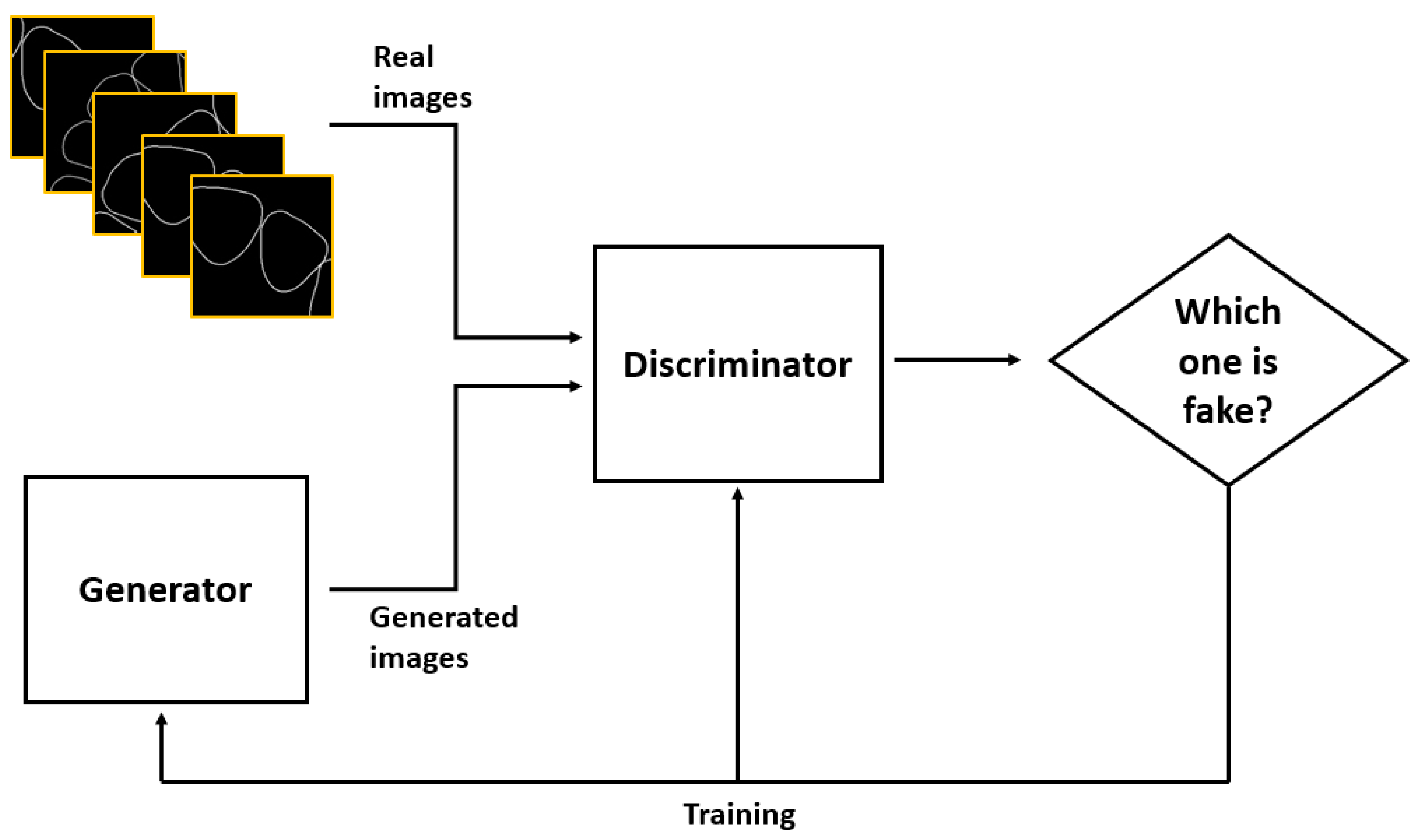
Research on artificial intelligence has recently been actively conducted. A generative adversarial network (GAN) is a type of artificial intelligence that method that learns a generative model and a discriminative model simultaneously. The system configuration of a GAN is described as follows (Figure 3). The generative model learns the distribution of data, and the discriminative model evaluate the data generated by the generative model. Next, the generative model then generates data such that an error when evaluating the learning model and an error when evaluating the generated model are similar. The generative model is briefly trained to induce a discrimination of the discriminative model.
1.3.2. Image Completion
Image completion is a technique used to remove and complete parts of an image that we want to restore. In this way, we can remove an unwanted part of an image and regenerate the occluded regions. Previously, there have been many approaches using patch-based methods [12,13,14,15]. However, the results were unsatisfactory owing to the complexity of the image pattern in various of objects, and it was difficult to increase the accuracy.
Methods using artificial intelligence have recently been studied. A context encoder is one such method and employs a convolutional neural network (CNN) [16,17]. Globally and locally consistent image completion (GLCIC) and Edge Connect also use artificial intelligence [18,19]. Whereas a context encoder is based on a CNN, a GLCIC and Edge Connect are based on a GAN. Among all methods described above, Edge Connect achieves the best accuracy [19]. Therefore, in this study, we employed an Edge Connect as the image completion method.
1.3.3. Goals
Various studies have been made to solve the difficulties of segmentation, and automation has resulted in a reduction in working time. However, both methods using the tooth boundary and tooth region do not solve the occlusion problem. In this study, we aim to solve the occlusion problem by pre-processing dental scan data using the image completion method. Additionally, using this approach, we expect to improve the tooth segmentation accuracy.
2. Proposed Method
2.1. Overview
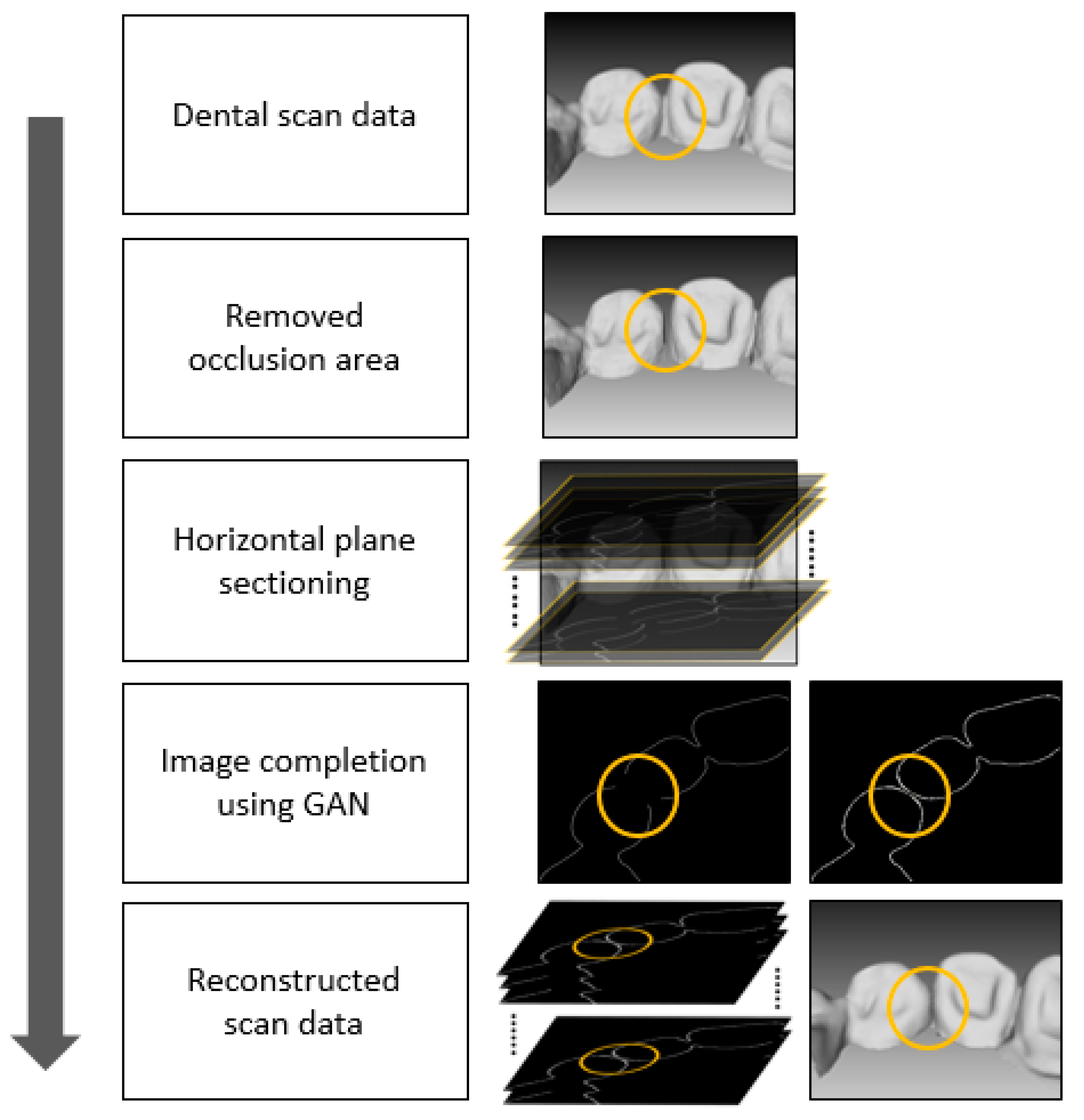
The system used to solve the occlusion problem of dental scan data when applying a GAN can be introduced through three steps. The first step is to remove the occlusion areas of the dental scan data. The next step is to complete the images on each plane. The final step is to stack the images from the previous step and reconstruct the dental scan data. The figure below depicts an overview of the proposed method (Figure 4).
2.2. Reconstruction of Dental Scan Data
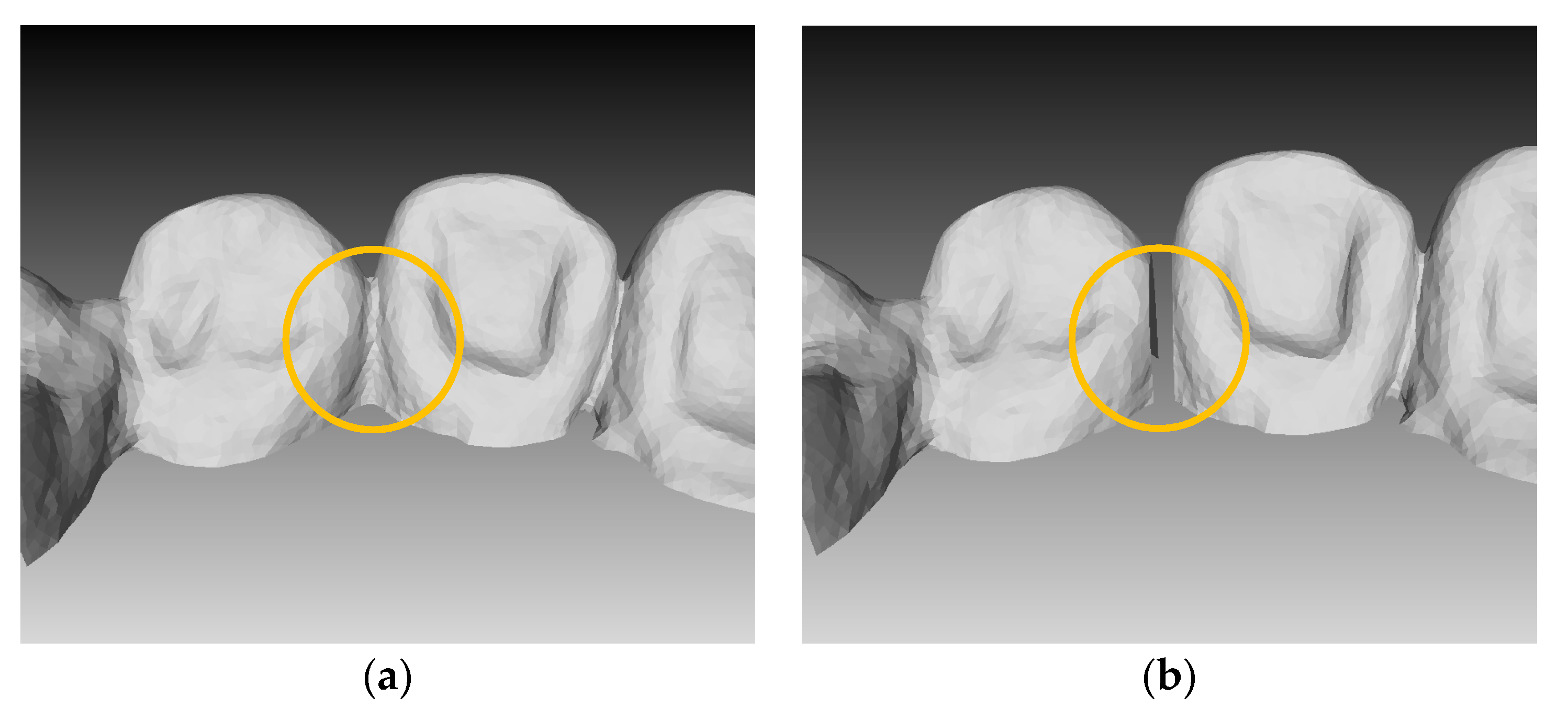
The reconstruction process is as follows. First, the occlusion area is specified by visual inspection of the interdental area whereby the intraoral scan data are not captured accurately. Here, the removed occlusion areas will be used as masks and the location must be saved. The occlusion area was deleted, and this removed area must be reconstructed. Figure 5 depicts images from before and after removing the occlusion area.
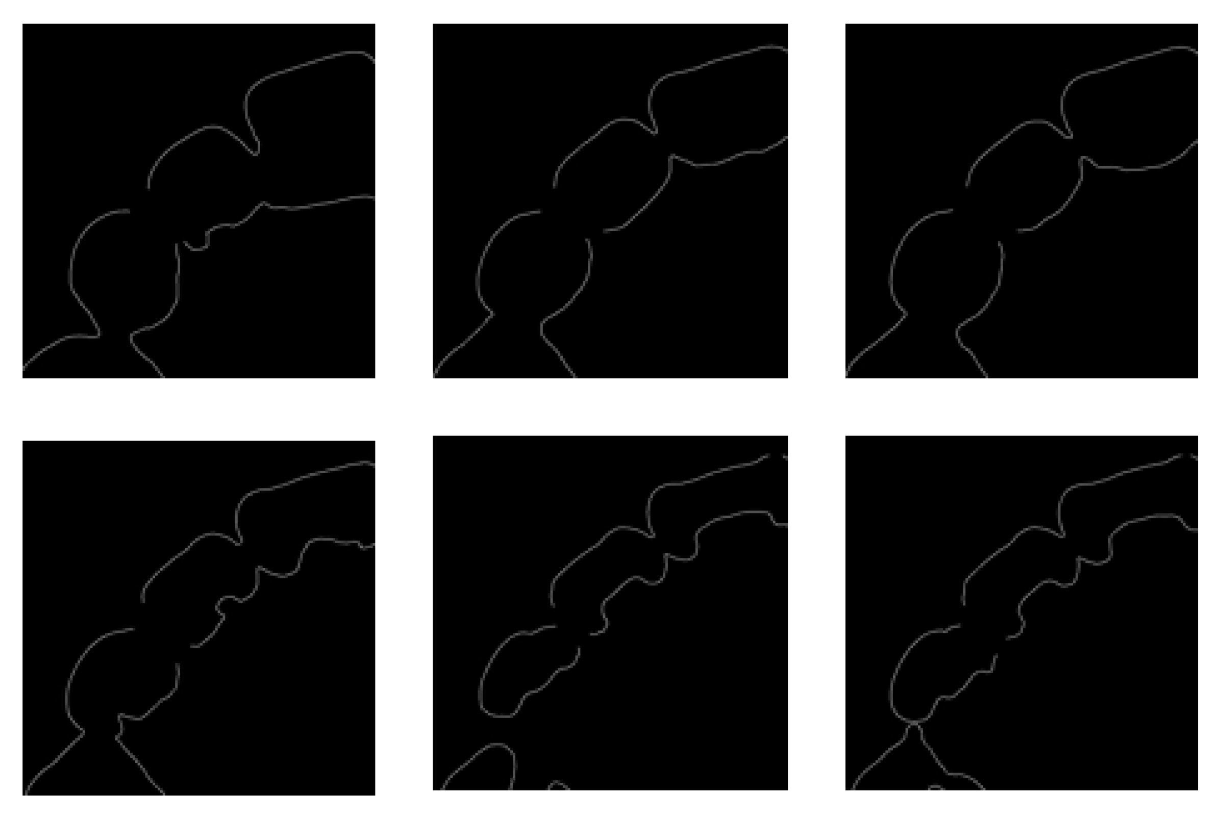
Next, dental scan data are sectioned at regular intervals using the horizontal plane direction. The more images we apply during the reconstruction at narrow intervals, the higher the accuracy that will be acquired, but the longer the computational time required. We used 0.1 mm intervals and achieved an image completion using 100 images per patient. The figures below show several images acquired using horizontal plane sectioning (Figure 6). Image completion is then conducted using a GAN (Figure 7).
Finally, the completed images are stacked using the previously saved location and height interval. We use only the restored area, as indicated by the circle in Figure 7. When the location of the reconstructed part is unknown, a registration should be applied using an algorithm, such as the iterative closest point (ICP) [20], which can cause additional errors. After the images are stacked to achieve a 3D image, the image is merged with the data where the occlusion areas have been removed. The process is completed through remeshing. The figures below illustrate the merging process (Figure 8).
2.3. Training GAN
Edge Connect, which adds the contour reconstruction described above, requires two learning processes. One process is contour restoration learning and the other is image completion learning. Both processes use a GAN. The neural networks of the generative model and the discriminative model used in this study are similar to those of Edge Connect. In detail, a generative model follows the super-resolution architecture [21,22], and the discriminative model follows a 70 × 70 patch GAN architecture [23,24].
2.3.1. Data Preparation
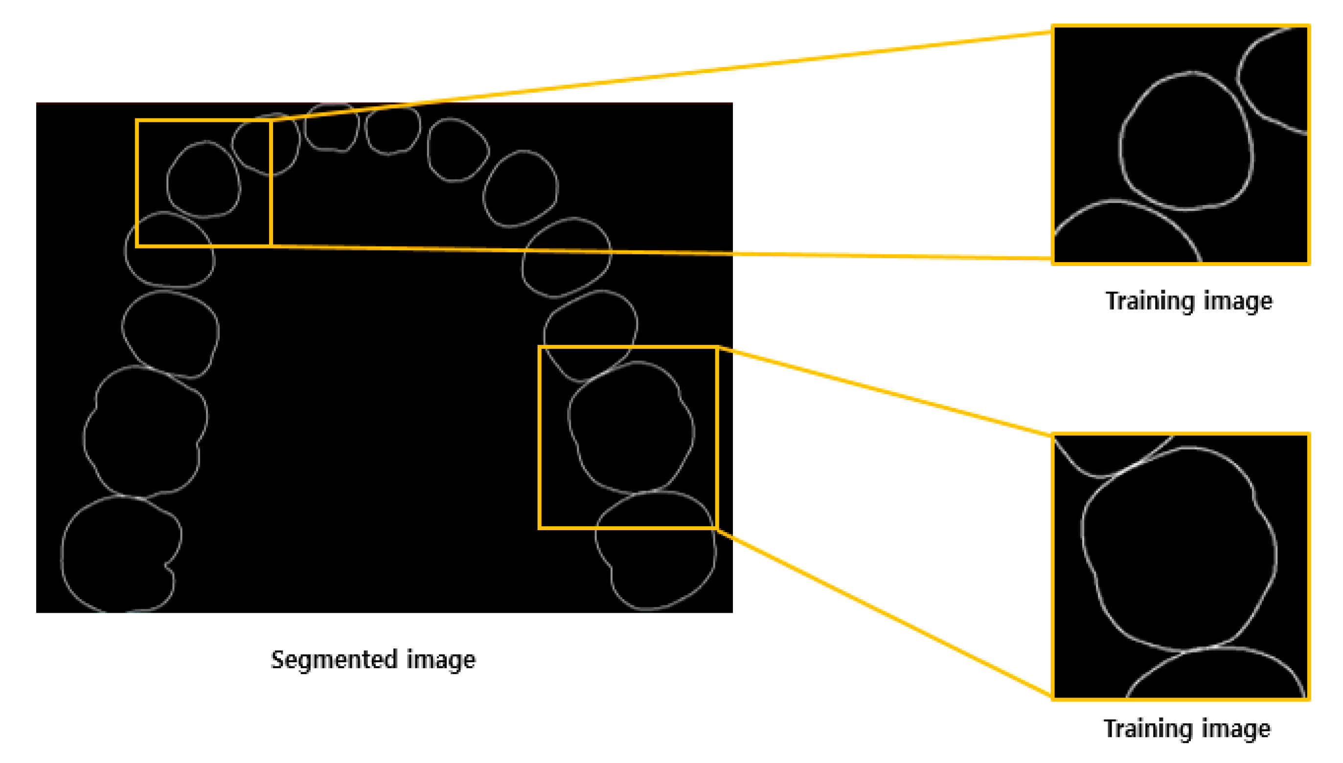
This study was approved by the Institutional Review Board of Korea University Anam Hospital (2019AN0470). Intraoral scan data of ten patients, who had taken a digital impression as part of an orthodontic diagnosis, were exported and segmented by a trained dental technician. The scans were acquired by one orthodontist by using the Trios 3 intraoral scanner (3Shape, Denmark). The figure below depicts the dental scan data after the segmentation process and one of the horizontal plane images (Figure 9).
The area to be used for learning is cropped into a 256 (px) × 256 (px) square in the horizontally sectioned images, as shown in (b) of Figure 9. In this study, we used 10,000 cropped images for training the GAN. The ratio of the training, validation, and test sets was 28:1:1. In general, approximately 100,000 images are used for training complex images, such as CelebA or Paris Street View. However, in the case of tooth data, the images are not complicated and can be trained using only 10,000 images. The training data was organized such that the tooth images were contained. Figure 10 shows the process of image cropping.
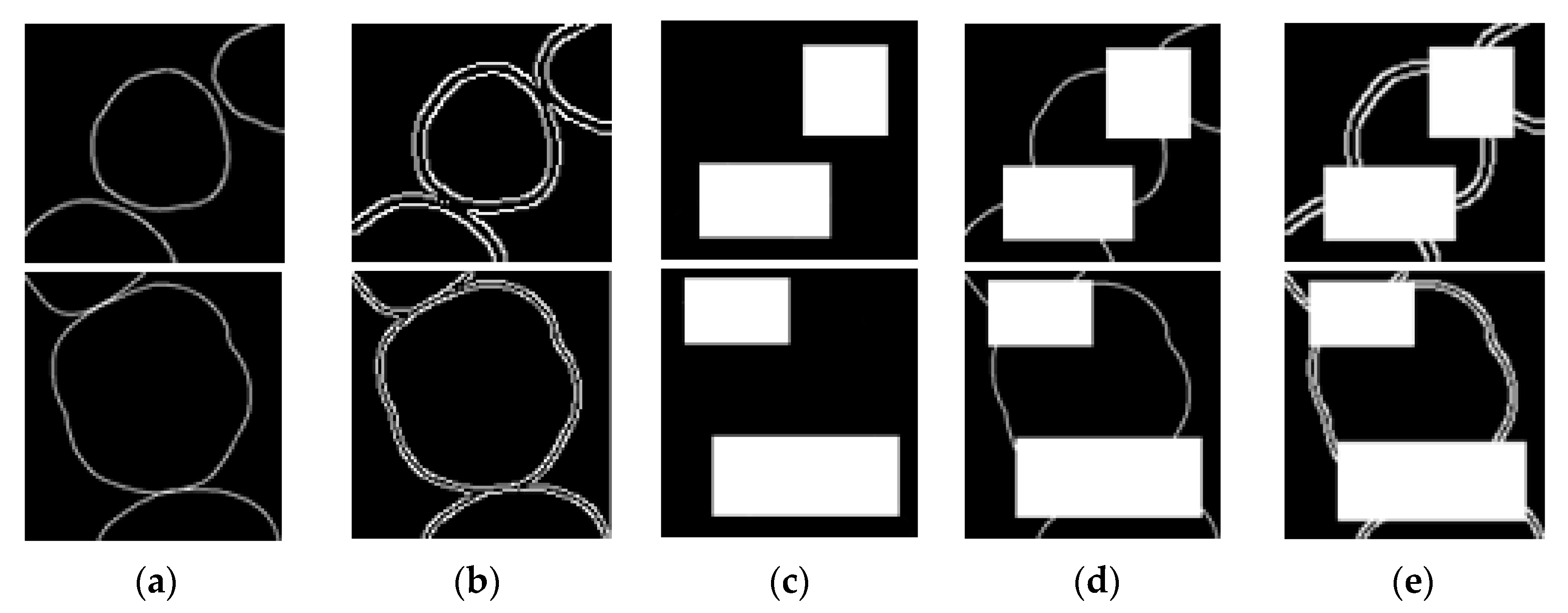
Five types of data are prepared: Cropped images, edge images, masks, masked images, and masked edge images. The cropped images can already be seen as edge images, but using edge images of the cropped images is important in terms of accuracy. We can apply the Edge Connect method when we consider only the cropped images as a picture, and not the edge images. For the edge images, we used the Canny edge detector with a threshold of 0.5 [25]. We determined the masks based on the dental spaces, where occlusions mainly occur. Any mask shape can be used, and the mask only needs to cover the areas where an occlusion is expected to occur. Herein, we used a rectangular shape. Figure 11 illustrates a few examples of the five types of data.
2.3.2. Training Steps
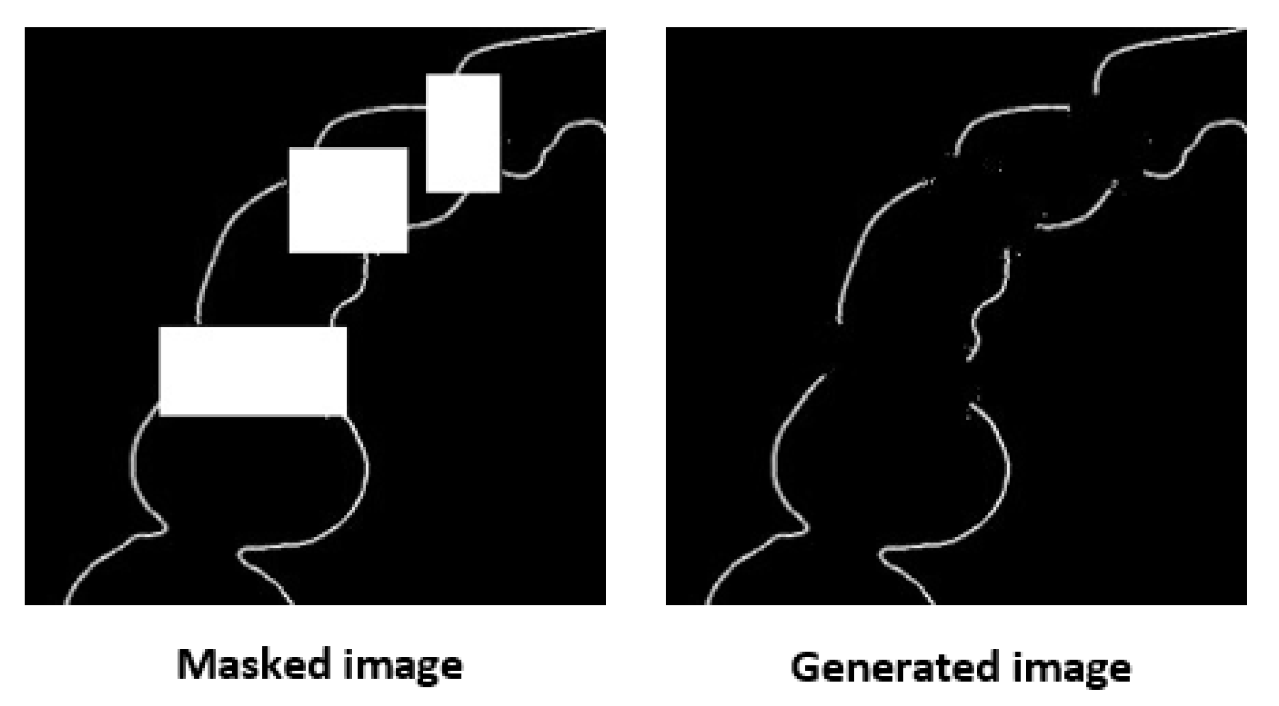
The first step is to pre-train the edge model. Among the data in Figure 11, we used masks (Figure 11c), masked images (Figure 11d), and masked edges (Figure 11e) as input images. Output images are full edge images, and the target images of the output are depicted in Figure 11b. The goal of this process is to pre-train only the edge model. Figure 12 depicts an image generated using the pre-trained edge model. As depicted in the figure, it is difficult to make an accurate image by training the edge alone.
The second step is to pre-train the image completion model. During this process, we use the edge images, masks, and masked images depicted in Figure 11b–d as input images, respectively. The output images are full images and the target images of the output are indicated in Figure 11a. The goal of this process is to pre-train only the image completion model. This is a separate learning process rather than an additional training of the model trained in the first step. The following is an image created by the pre-trained image completion model (Figure 13). The high mask ratio on the test image reduces the accuracy of the image completion.
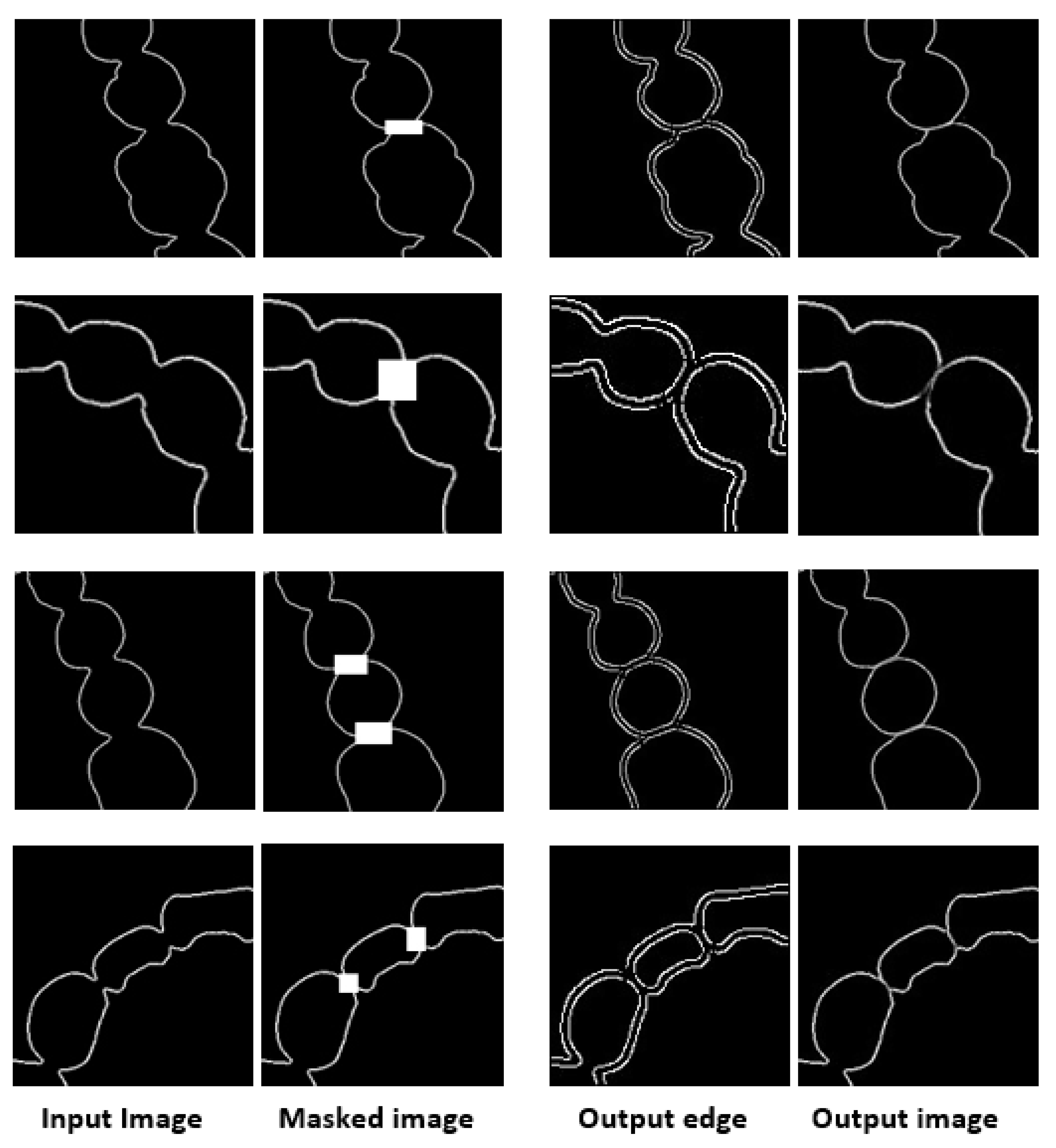
The third step is to train images by using the two pre-trained models, the edge model and the image completion model. First, we used the pre-trained edge model to make edge images. Then we used the generated edge images, the masks from Figure 11c, and masked images from Figure 11d as the input. The output images are restored images, and the target images are depicted in Figure 11a. We used the weight file of the pre-trained image completion model to fine-tune the edge connect model. Figure 14 is an image generated after the last step of training. We can now see the reason why the edge images are made. Figure 14 shows that restoring images by simultaneously using both, the edge generative model and the image completion model delivers better results.
3. Results and Discussion
3.1. Result of Image Completion
We applied the trained GAN using the proposed method to the actual tooth image completion. Overall, it took 4 days for training: Steps 1 and step 2 required 1 day each, and step 3 took 2 days. We used a personal computer with an i7-6700 (3.4 GHz) processor, 24 GB of RAM, and an RTX 2080 Ti GPU. The figures below show some examples of the results (Figure 15).
We used the structural similarity index (SSIM) [26] and peak signal-to-noise ratio (PSNR) [27] to quantitatively measure the training result of a GAN. The SSIM is a measure of the difference between the ground truth image and the image being compared. The value closer to 1 indicates better results. The PSNR is a measure of the sharpness and uses the difference in noise between the ground truth image and the restored image. The table below presents the accuracy measured by the SSIM (Table 1), which we classified according to the mask ratios to assess the effect on the image completion. The closer the value is to 1, the better the result.
For a more intuitive explanation of the SSIM, images with values of 0.75–0.95 among those used in the experiments are shown at 0.05 intervals (Figure 16). The left side shows the ground truth images, and the right side shows the restored images. From a value of 0.85 and above, we can see the edge lined up, and a value above 0.9 is similar to that of the ground truth images.
The following is the result measured based on the PSNR (Table 2). Higher values indicate better results. The images used in the experiment are 16.42 at minimum and 28.27 at maximum.
As with the SSIM, among the images used in the experiment, images with a PSNR of 16–28 are shown at three intervals (Figure 17). The edges on the left are the ground truth images and the images on the right are the generated images. When the PSNR is less than 20, we can see that the edge is broken or missing. A small amount of noise occurs from above 22, although this is similar to the ground truth images.
The SSIM and PSNR differed significantly according to the mask sizes. Figure 18 and Figure 19 show the changes according to the mask sizes. We can see this visually in the figures below (Figure 20). The smaller the mask size is the better. However, there is a minimum mask size of an image because the mask must cover the occlusion area. Therefore, the use of large and high-resolution images lead to better results. However, computer performance was limited, and we used cropped images.
In this study, we used images with an SSIM of over 0.9 and a PSNR of over 22 for 3D reconstruction. Overall, when the mask size is less than 10%, 95% of the images obtained are available for 3D reconstruction. It took 0.1 s for an image completion, and we used 100 slices of both the maxilla and mandible. We conducted the image completion five times per slice. Therefore, the entire image completion process took approximately 100 s.
3.2. Results of Tooth Segmentation
3.2.1. Tooth Model
A tooth pin model of a malocclusion patient was fabricated for the testing of the segmentation algorithm (Figure 21). This model allows each tooth to be removed and replaced to its original position from the tooth model base. Therefore, it is suitable for use in our experiments because each tooth can be removed and scanned individually with no occlusions. The scan data of each tooth were used as the ground truth.
3.2.2. Accuracy Measurement Process
Two data are needed for an accurate measurement. One is the entire scan data and the other is separated scan data. The former has occlusion areas, whereas, the latter does not. Therefore, we used the separated scan data as the ground truth. Next, we conducted segmentation on the entire scan data using the conventional and proposed methods (Figure 22). Then, we measured the accuracy of the separated scan data as the ground truth and compared it with the tooth data segmented by each method.
3.2.3. Measurement Accuracy Results
Jung et al. [28] proposed an effective registration technique, which we used for the registration of the three data types. After the registration, we used Geomagic software (2012, Ping Fu, Herbert Edelsbrunner, Morrisville, NC, USA) to compare the distances between the data. We set the ground truth data as a mesh and the data segmented by each method as point clouds. The data segmented by each method were then sampled for a constant number of points. We classified the results into four tooth types, namely, incisor, canine, premolar, and molar, and measured the average mean distance between the point cloud and the mesh. The table below presents the results (Table 3). The conventional method indicates the manual segmentation using the snake. The proposed method indicates segmentation by using GAN.
The mean distance between the point cloud and the mesh for each method is displayed in Table 3. The above results show that the proposed method is approximately 0.004 mm more accurate than the conventional method, and this difference was significantly different (p = 0.033).
4. Conclusions
In this study, we proposed an automated method to reconstruct the missing data in the interdental area of teeth, scanned using an intraoral scanner by applying a GAN. A limitation is that the masks were manually applied to the occlusion area, therefore, some of the normal scan data may have been removed. A further study carried out to automatically detect the occlusion area would define the masks with higher precision and increase the accuracy of segmentation. Nonetheless, based on our results on the dimensional accuracy of the segmented teeth, it can be inferred that the segmentation method for full arch intraoral scan data is as accurate as a manual segmentation method, in addition to being effective and time saving. This automatic segmentation tool can be used to facilitate the digital setup process in orthodontic treatment.
Author Contributions
Conceptualization, T.K.; data curation, D.K.; formal analysis, T.K.; investigation, M.C.; Methodology, T.K. and Y.C.; project administration, M.C.; resources, Y.-J.K.; supervision, Y.-J.K. and M.C.; validation, T.K.; visualization, T.K.; writing—original draft, T.K.; writing—review and editing, Y.-J.K. All authors have read and agreed to the published version of the manuscript.
Funding
This research received no external funding.
Acknowledgments
We are grateful to the Department of Orthodontics, Korea University Anam Hospital for providing the patients’ scan data and the tooth pin model.
Conflicts of Interest
The authors declare no conflicts of interest.
References
- Kesling, H. The diagnostic setup with consideration of the third dimension. Am. J. Orthod. Dentofac. Orthop. 1956, 42, 740–748. [Google Scholar] [CrossRef]
- Barreto, M.S.; Faber, J.; Vogel, C.J.; Araujo, T.M. Reliability of digital orthodontic setups. Angle Orthod. 2016, 86, 255–259. [Google Scholar] [CrossRef] [PubMed] [Green Version]
- Im, J.; Cha, J.Y.; Lee, K.J.; Yu, H.S.; Hwang, C.J. Comparison of virtual and manual tooth setups with digital and plaster models in extraction cases. Am. J. Orthod. Dentofac. Orthop. 2014, 145, 434–442. [Google Scholar] [CrossRef] [PubMed]
- Chen, B.T.; Lou, W.S.; Chen, C.C.; Lin, H.C. A 3D scanning system based on low-occlusion approach. In Proceedings of the Second International Conference on 3-D Digital Imaging and Modeling (Cat. No. PR00062), Ottawa, ON, Canada, 8 October 1999; IEEE: Piscataway, NJ, USA, 1999; pp. 506–515. [Google Scholar]
- Shlafman, S.; Tal, A.; Katz, S. Metamorphosis of polyhedral surfaces using decomposition. In Computer Graphics Forum; Blackwell Publishing, Inc.: Oxford, UK, 2002; pp. 219–228. [Google Scholar]
- Mangan, A.P.; Whitaker, R.T. Partitioning 3D surface meshes using watershed segmentation. IEEE Trans. Vis. Comput. Graph. 1999, 5, 308–321. [Google Scholar] [CrossRef] [Green Version]
- Lee, Y.; Lee, S.; Shamir, A.; Cohen-Or, D.; Seidel, H.P. Mesh scissoring with minima rule and part salience. Comput. Aided Geom. Des. 2005, 22, 444–465. [Google Scholar] [CrossRef]
- Zanjani, F.G.; Moin, D.A.; Claessen, F.; Cherici, T.; Parinussa, S.; Pourtaherian, A.; Zinger, S. Mask-MCNet: Instance segmentation in 3D point cloud of intra-oral scans. In International Conference on Medical Image Computing and Computer-Assisted Intervention; Springer: Cham, Switzerland, 2019; pp. 128–136. [Google Scholar]
- Podolak, J.; Shilane, P.; Golovinskiy, A.; Rusinkiewicz, S.; Funkhouser, T. A planar-reflective symmetry transform for 3D shapes. ACM Trans. Graph. (TOG) 2006, 25, 549–559. [Google Scholar] [CrossRef]
- Lai, Y.K.; Hu, S.M.; Martin, R.R.; Rosin, P.L. Fast mesh segmentation using random walks. In Proceedings of the 2008 ACM Symposium on Solid and Physical Modeling, New York, NY, USA, 2–4 June 2008; ACM: New York, NY, USA, 2008; pp. 183–191. [Google Scholar]
- Kronfeld, T.; Brunner, D.; Brunnett, G. Snake-based segmentation of teeth from virtual dental casts. Comput. Aided Des. Appl. 2010, 7, 221–233. [Google Scholar] [CrossRef] [Green Version]
- Barnes, C.; Shechtman, E.; Goldman, D.B.; Finkelstein, A. The generalized patchmatch correspondence algorithm. In European Conference on Computer Vision; Springer: Berlin/Heidelberg, Germany, 2010; pp. 29–43. [Google Scholar]
- Darabi, S.; Shechtman, E.; Barnes, C.; Goldman, D.B.; Sen, P. Image melding: Combining inconsistent images using patch-based synthesis. ACM Trans. Graph. 2012, 31, 82-1–82-10. [Google Scholar] [CrossRef]
- Huang, J.B.; Kang, S.B.; Ahuja, N.; Kopf, J. Image completion using planar structure guidance. ACM Trans. Graph. (TOG) 2014, 33, 129. [Google Scholar] [CrossRef]
- Simakov, D.; Caspi, Y.; Shechtman, E.; Irani, M. Summarizing visual data using bidirectional similarity. In Proceedings of the 2008 IEEE Conference on Computer Vision and Pattern Recognition, Anchorage, AK, USA, 23–28 June 2008; IEEE: Piscataway, NJ, USA, 2008; pp. 1–8. [Google Scholar]
- Köhler, R.; Schuler, C.; Schölkopf, B.; Harmeling, S. Mask-specific inpainting with deep neural networks. In German Conference on Pattern Recognition; Springer: Cham, Switzerland, 2014; pp. 523–534. [Google Scholar]
- Ren, J.S.; Xu, L.; Yan, Q.; Sun, W. Shepard convolutional neural networks. In Advances in Neural Information Processing Systems; The MIT Press: Cambridge, MA, USA, 2015; pp. 901–909. [Google Scholar]
- Iizuka, S.; Simo-serra, E.; Ishikawa, H. Globally and locally consistent image completion. ACM Trans Graph. (ToG) 2017, 36, 107. [Google Scholar] [CrossRef]
- Nazeri, K.; Ng, E.; Joseph, T.; Qureshi, F.; Ebrahimi, M. Edgeconnect: Generative image inpainting with adversarial edge learning. arXiv 2019, arXiv:1901.00212. [Google Scholar]
- Besl, P.J.; Mckay, N.D. Method for registration of 3-D shapes. In Sensor Fusion IV: Control Paradigms and Data Structures; International Society for Optics and Photonics: Bellingham, WA, USA, 1992; pp. 586–606. [Google Scholar]
- Sajjadi, M.S.; Scholkopf, B.; Hirsch, M. Enhancenet: Single image super-resolution through automated texture synthesis. In Proceedings of the IEEE International Conference on Computer Vision, Venice, Italy, 22–29 October 2017; pp. 4491–4500. [Google Scholar]
- Waleed Gondal, M.; Scholkopf, B.; Hirsch, M. The unreasonable effectiveness of texture transfer for single image super-resolution. In Proceedings of the European Conference on Computer Vision (ECCV), Munich, Germany, 8–14 September 2018. [Google Scholar]
- Isola, P.; Zhu, J.Y.; Zhou, T.; Efros, A.A. Image-to-image translation with conditional adversarial networks. In Proceedings of the IEEE Conference on Computer Vision and Pattern Recognition, Honolulu, HI, USA, 21–26 July 2017; pp. 1125–1134. [Google Scholar]
- Zhu, J.Y.; Park, T.; Isola, P.; Efros, A.A. Unpaired image-to-image translation using cycle-consistent adversarial networks. In Proceedings of the IEEE International Conference on Computer Vision, Venice, Italy, 22–29 October 2017; pp. 2223–2232. [Google Scholar]
- Canny, J. A computational approach to edge detection. IEEE Trans. Pattern Anal. Mach. Intell. 1986, 6, 679–698. [Google Scholar] [CrossRef]
- Wang, Z.; Bovik, A.C.; Sheikh, H.R.; Simoncelli, E.P. Image quality assessment: From error visibility to structural similarity. IEEE Trans. Image Process. 2004, 13, 600–612. [Google Scholar] [CrossRef] [PubMed] [Green Version]
- De Boer, J.F.; Cense, B.; Park, B.H.; Pierce, M.C.; Tearney, G.J.; Bouma, B.E. Improved signal-to-noise ratio in spectral-domain compared with time-domain optical coherence tomography. Opt. Lett. 2003, 28, 2067–2069. [Google Scholar] [CrossRef] [PubMed]
- Jung, S.; Song, S.; Chang, M.; Park, S. Range image registration based on 2D synthetic images. Comput. Aided Des. 2018, 94, 16–27. [Google Scholar] [CrossRef]
Figure 1.
Occlusion areas of dental scan data.

Figure 2.
Segmentation using a snake: (a) Initial; and (b) modified positions using snake.

Figure 3.
Overview of generative adversarial network (GAN).

Figure 4.
Overview of the proposed method.

Figure 5.
Example of removing the occlusion area: (a) before and (b) after removal.

Figure 6.
Examples of horizontal plane sectioning.

Figure 7.
Examples of image completion.

Figure 8.
Example after reconstruction: (a) Dental scan data with occlusion area removed, (b) reconstructed data by stacking images, and (c) dental scan data by merging (a,b).
Figure 8.
Example after reconstruction: (a) Dental scan data with occlusion area removed, (b) reconstructed data by stacking images, and (c) dental scan data by merging (a,b).

Figure 9.
Data after tooth segmentation: (a) 3D and (b) horizontal views of the data.

Figure 10.
Cropping images from segmented data.

Figure 11.
Example of five types of training data: (a) cropped images from Figure 10, (b) edge images from (a), (c) masks, (d) masked images of (a), and (e) masked edges of (a).
Figure 11.
Example of five types of training data: (a) cropped images from Figure 10, (b) edge images from (a), (c) masks, (d) masked images of (a), and (e) masked edges of (a).

Figure 12.
Image generated using the pre-trained edge model.

Figure 13.
Image generated using the pre-trained image completion model.

Figure 14.
Image generated after the last training step.

Figure 15.
Some examples of generated images.


Figure 16.
Images of various structural similarity index (SSIMs).

Figure 17.
Images of various PSNRs.

Figure 18.
Effect of mask sizes on the SSIM.

Figure 19.
Effect of mask sizes on the PSNR.

Figure 20.
Results of different mask sizes.

Figure 21.
Tooth pin model.

Figure 22.
(a) Data obtained through segmentation obtained using the proposed and (b) conventional methods.
Figure 22.
(a) Data obtained through segmentation obtained using the proposed and (b) conventional methods.


Table 1.
Evaluation using structural similarity index (SSIM).
| Mask | Incisor | Canine | Premolar | Molar |
|---|---|---|---|---|
| 0–10% | 0.921 | 0.918 | 0.911 | 0.923 |
| 10–20% | 0.915 | 0.911 | 0.906 | 0.913 |
| 20–30% | 0.885 | 0.883 | 0.879 | 0.894 |
| 30–40% | 0.819 | 0.822 | 0.839 | 0.859 |
Table 2.
Evaluation based on PSNR.
| Mask | Incisor | Canine | Premolar | Molar |
|---|---|---|---|---|
| 0–10% | 26.68 | 24.42 | 24.71 | 26.27 |
| 10–20% | 25.82 | 24.19 | 23.69 | 25.07 |
| 20–30% | 22.72 | 22.57 | 21.62 | 23.33 |
| 30–40% | 19.49 | 19.78 | 19.71 | 21.93 |
Table 3.
Average mean distance between the point cloud and mesh.
| Method | Mean Distance (mm) | p |
|---|---|---|
| Conventional | 0.031 ± 0.008 | 0.033 |
| Proposed | 0.027 ± 0.007 |
p, p-value for independent t-test.
© 2020 by the authors. Licensee MDPI, Basel, Switzerland. This article is an open access article distributed under the terms and conditions of the Creative Commons Attribution (CC BY) license (http://creativecommons.org/licenses/by/4.0/).
Share and Cite
MDPI and ACS Style
Kim, T.; Cho, Y.; Kim, D.; Chang, M.; Kim, Y.-J. Tooth Segmentation of 3D Scan Data Using Generative Adversarial Networks. Appl. Sci. 2020, 10, 490. https://doi.org/10.3390/app10020490
AMA Style
Kim T, Cho Y, Kim D, Chang M, Kim Y-J. Tooth Segmentation of 3D Scan Data Using Generative Adversarial Networks. Applied Sciences. 2020; 10(2):490. https://doi.org/10.3390/app10020490
Chicago/Turabian StyleKim, Taeksoo, Youngmok Cho, Doojun Kim, Minho Chang, and Yoon-Ji Kim. 2020. "Tooth Segmentation of 3D Scan Data Using Generative Adversarial Networks" Applied Sciences 10, no. 2: 490. https://doi.org/10.3390/app10020490
Note that from the first issue of 2016, this journal uses article numbers instead of page numbers. See further details here.