Control Points Selection Based on Maximum External Reliability for Designing Geodetic Networks

Abstract

A set of stable and identifiable points—known as control points—are interconnected by direction, distance or height differences measurements form a geodetic network. Geodetic networks are used in various branches of modern science, such as monitoring the man-made structures, analysing the crustal deformation of the Earth, establishing and maintaining a geospatial reference frame, mapping, civil engineering projects and others. One of the most crucial components for ensuring the network quality is Geodetic Network Design. The design of a geodetic network depends on its purpose. In this paper, an automatic procedure for selection of control points is proposed. The goal is to find the optimum control points location so that the maximum influence of an anomaly measurement (outlier) on the coordinates of the network is minimum. Here, the concept of Minimal Detectable Bias defines the size of the outlier and its propagation on the network coordinates is used to describe the external reliability. The proposed procedure was applied to design a levelling network. Two scenarios were investigated: design of a network with one control point (minimally constrained levelling network) and another with two control points (over-constrained levelling network). The centre of the network was the optimum position to set the control point. Results for that network reveal that the centre of the network was the optimum position to set the control point for the minimal constraint case, whereas the over-constraint case were those with less line connections. We highlight that the procedure is a generally applicable method.

1. Introduction

A geodetic network consists of a set of stable and identifiable points located on the Earth’s surface or near it [1]. Their positions are associated with a coordinate reference system. These points are referred to control points. These control points provide the common basis for surveying and mapping activities. of particular importance is the densification of a geodetic network. In that case, new geodetic networks are established based on an existing network. In other words, new points are often tied to previously established control points.

If we want to determine the coordinates of that new points, measurements based on directions, distances, height differences and/or space-based geodetic techniques, such as Global Navigation Satellite Systems (GNSS), should be performed between the new points and the existing control points (now we just refer “existing control points” to as control points). In most cases of geodetic networks, the measurements bear a known linear relationship with the unknown parameters. In other words, the mathematical model that relates measurements to parameters is linear. In that case, the coordinates of new points are unknown parameters, whereas the coordinates of control points are constraints on the mathematical model. Details about constraints can be verified in [2].

The coordinates of the new points are often computed from the Least-Squares Estimation (LSE). In other words, we seek to find the coordinates of the new points that minimises the sum-of-squares of the residuals. The residuals is the difference between the observed values and the estimated (or expected) values of the measurements [3,4,5].

A step prior to the deployment of a geodetic network is the Geodetic Network Design. The quality of a geodetic network is characterised by its precision, reliability, and cost [6,7]. The covariance matrix of the least-squares parameters is associated with the degree of the network precision. There is also the internal and external reliability of a geodetic network, which were both introduced by [4]. Internal reliability refers to the ability of a network to detect outliers in the set of observations, and external reliability refers to the effect of the undetectable outliers on the estimated parameters. Here, outlier is defined according to [8]: “An outlier is an measurement that is so probably caused by a gross error that it is better not used or not used as it is”. The cost is related to the effort required to implement the design and related expenses.

There is not the best geodetic network, but the optimal geodetic network. Designing a geodetic network in the optimal sense involves designing an optimal configuration for the network (e.g., selection of the position of network control points). Optimal design problem of a geodetic network was widely investigated since the pioneering work of [9,10]. Since then, several works were described in detail in papers published in scientific journals (see e.g., [1,6,7,11,12,13,14,15,16,17,18,19]). Details about the orders of design is outside of discussion in this paper. However, details can be found in [10,11]. In this paper, we provide an automatic procedure to design a geodetic network in terms of reliability. Here, we use the reliability theory for designing geodetic networks. The reliability theory becomes a fundamental part of modern data analysis [1,20,21,22,23]. This is due to [3,4].

Generally, the random measurement errors in a system are unavoidable. However, the presence of an outlier in the dataset can jeopardise the reliability level of the system. To detect a possible outlier, Baarda [4] introduced the Data Snooping procedure for the detection of a single outlier in linear(ised) models. Most of conventional geodetic studies have a chapter on Baarda’s data snooping procedure, e.g., [5,24]. Data snooping has become very popular and is routinely used in adjustment computations [25]. Although introduced in the context of geodetic networks, Data Snooping is a generally applicable method of outlier detection in both univariate and multivariate approaches [26].

Data snooping is a procedure based on hypothesis testing, which consists of screening each individual observation for a possible outlier. The test statistic associated with Data Snooping is given by a normalised least-squares residuals. That test, known as Baarda’s w-test, can also be derived as a particular case of the generalised likelihood ratio test [27]. Baarda’s w-test makes a decision between the null ${\mathcal{H}}_0$ (model in the absence of an outlier) and a single alternative hypothesis ${\mathcal{H}}_A$ (model in the presence of an outlier). In that case, rejection of ${\mathcal{H}}_0$ automatically implies acceptance of ${\mathcal{H}}_A$, and vice-versa [21,22,28]. Here, we restrict ourselves to the only one single alternative hypothesis. In the case where multiple alternative hypotheses are in play, the readers can consult, for example, [22,26].

Since Data Snooping is based on a hypothesis testing, it may lead to a errors decision. There is the probability of rejecting a true null hypothesis ${\mathcal{H}}_0$, which is well-known type I decision error (denoted by “$\alpha$”). The probability level $\alpha$ (known as significance level of a test) defines the size of a test and is often known as “false alarm probability” [29]. On the other hand, there is the probability of rejecting a true alternative hypothesis ${\mathcal{H}}_A$ (type II decision error—‘missed detection’, denoted by “$\beta$”). Based on the probability levels $\alpha$ and $\beta$, Baarda [3,4] derived the concept of Minimal Detectable Bias (MDB)—the term given [30]. The MDB is the additional bias (or are the additional biases) in the parameters vector that can be detected by the w-test with a certain probability of $1-\beta$. The MDB can be computed before actual measurements were carried out, using only a functional model and the expected stochastic properties of the data [5]. In addition, it is possible to describe the influences of the MDBs on the geodetic network coordinates (i.e., on the parameters). The set of MDBs describes the internal reliability, whereas their propagation on the parameters is said to describe the external reliability [31].

The internal and external reliability, therefore, are very useful tool to assess the magnitude of possible errors that can be detected during the pre-processing of the data. For this reason, the concept of the internal (quantified by MDB) and external reliability can be applied during the design stage of geodetic network. In this context, the goal is to apply the reliability theory for designing geodetic network. The quality criterion considered here is based on the external reliability. The position of the control point of geodetic network is selected so that the maximum influence of an MDB on the coordinates of the network points is minimum. A levelling network is used as an example of application of the proposed method. Here, we consider a scenario where the observations of the network have the same uncertainties and another with different uncertainties. We also consider the case of minimally constrained (one control point in the case of levelling network) and over-constrained network (two control points).

2. Conventional Reliability Theory

The null hypothesis ${\mathcal{H}}_0$ corresponds to a model in the absence of outliers. Thus, the null hypothesis of the standard Gauss–Markov model in linear or linearised form is given by [24]:

$${\mathcal{H}}_0:\mathbb{E}\left\{\mathit{y}\right\}=\mathit{A}\mathit{x}+\mathbb{E}\left\{\mathit{e}\right\}=\mathit{A}\mathit{x},$$

(1)

where $\mathbb{E}\{.\}$ is the expectation operator, $\mathit{y}\in {\mathbb{R}}^n$ the vector of measurements, $\mathit{A}\in {\mathbb{R}}^{n\times u}$ the Design Matrix) (also referred as Jacobian matrix) of full rank $u$, $\mathit{x}\in {\mathbb{R}}^u$ the unknown parameter vector, and $\mathit{e}\in {\mathbb{R}}^n$ the unknown vector of measurement errors.

Typically, it is assumed that the errors of the good measurements are normally distributed with expectation zero [32], i.e.,:

$$\mathit{e}\sim \mathit{N}(\mathbf{0},{\mathit{Q}}_{\mathit{e}}),$$

(2)

with a known positive definite symmetric covariance matrix ${\mathit{Q}}_{\mathit{e}}\in {\mathbb{R}}^{n\times n}$. Here, we confine ourselves to the case that $\mathit{A}$ and ${\mathit{Q}}_{\mathit{e}}$ have full column rank.

The redundancy (or degrees of freedom) of the model in Equation (1) is $r=n-u$. However, any model is only an approximation to the truth. This implies that we inevitably encounter misspecified models. In contrast to the ${\mathcal{H}}_0$, Baarda [4] introduced a mean shift model that defines the alternative hypothesis ${\mathcal{H}}_A$, also referred to as model misspecification, as follows:

$${\mathcal{H}}_A:\mathbb{E}\left\{y\right\}=\mathit{A}\mathit{x}+{\mathit{c}}_{\mathit{i}}{\nabla }_i+\mathbb{E}\left\{\mathit{e}\right\}=\left(\begin{array}{cc}\mathit{A}& {\mathit{c}}_{\mathit{i}}\end{array}\right)\left(\begin{array}{c}\mathit{x}\\ {\nabla }_i\end{array}\right),\forall i=1,\cdots ,n$$

(3)

where ${\mathit{c}}_{\mathit{i}}$ takes the form of a canonical unit vector with 1 as its ith entry and zeros elsewhere. The 1 value means that an ith bias parameter of magnitude ${\nabla }_i$ affects an ith measurement and 0 otherwise. We have, for instance, ${\mathit{c}}_{\mathit{i}}$=${\left(\begin{array}{cccccccc}0& 0& 0& \cdots & 1^{i_{th}}& 0& \cdots & 0\end{array}\right)}^T$. In other words, ${\mathit{c}}_{\mathit{i}}$ specifies the type of model error and ${\nabla }_i$ the size of the model error, or outlier.

The likelihood ratio test to test ${\mathcal{H}}_0$ against ${\mathcal{H}}_A$ is given by:

$$Accept{\mathcal{H}}_{0}if\left|{\mathit{w}}_{\mathit{i}}\right|\le k={\mathsf{\Phi }}^{-1}(1-\frac{\alpha }{2}),rejectotherwiseinfavourof{\mathcal{H}}_A$$

(4)

and the test statistics (known as Baarda’s w-test) are the normalised least-squares residuals given by [4]:

$${\mathit{w}}_{\mathit{i}}=\frac{{\mathit{c}}_{\mathit{i}}^T{\mathit{Q}}_{\mathit{e}}^{-1}\widehat{\mathit{e}}}{\sqrt{{\mathit{c}}_{\mathit{i}}^T{\mathit{Q}}_{\mathit{e}}^{-1}{\mathit{Q}}_{\widehat{\mathit{e}}}{\mathit{Q}}_{\mathit{e}}^{-1}{\mathit{c}}_{\mathit{i}}}}$$

(5)

According to (4) and (5), we have:

• $k$ is the critical value. The critical value $k$ is the the tabular value from the cumulative distribution function (cdf) of the standard normal $N(0,1)$ based on the chosen of a significance level $\alpha$. Because we perform a two-sided test of the form $|{\mathit{w}}_{\mathit{i}}|\le k$ we have $\alpha /2$. For example, for $\alpha =0.01$, we obtain $k=2.576$. In this case, if $|{\mathit{w}}_{\mathit{i}}|>2.576$ for some $y_i$ one may reject ${\mathcal{H}}_0$.
• ${\mathsf{\Phi }}^{-1}$ denotes the inverse of the normal cumulative distribution function.
• $\widehat{\mathit{e}}$ is the least-squares residuals vector under ${\mathcal{H}}_0$ and ${\mathit{Q}}_{\widehat{\mathit{e}}}$ the covariance matrix of the best linear unbiased estimator of $\widehat{\mathit{e}}$ under ${\mathcal{H}}_0$.

The decision rule in (4) says that if the test statistic $|w_{\mathit{i}}|$ in (5) is larger than some critical value $k$, i.e., a percentile of its probability distribution, then we reject the null hypothesis ${\mathcal{H}}_0$ in favour of the alternative hypothesis ${\mathcal{H}}_A$.

Because w-test is based on binary hypothesis testing, in which one decides between the null hypothesis ${\mathcal{H}}_0$ and a single alternative hypothesis ${\mathcal{H}}_A$, it may lead to type I decision error ($\alpha$) and type II decision error ($\beta$). The probability level $\alpha$ is the probability of rejecting the null hypothesis when it is true, whereas $\beta$ is the probability of failing to reject the null hypothesis when it is false. The complements of $\alpha$ and $\beta$ are well-known confidence level (CL) and the statistical power ($\gamma$), respectively. The first deals with the probability of accepting a true null hypothesis; the second, with the probability of correctly accepting the alternative hypothesis. In other words, we have $CL=1-\alpha$ and $\gamma =1-\beta$.

The normalised least-squares residual $w_i$ follows a standard normal distribution with the expectation that $\mu =0$ if ${\mathcal{H}}_0$ holds true. On the other hand, if the system is contaminated with a single error at the ith position of the dataset, there is an outlier that causes the expectation of $w_i$ to become $\mu >0$. The effect can be best understood using the non-central chi-squared distribution with one degree of freedom (i.e., for a single outlier). Under the alternative hypothesis ${\mathcal{H}}_A$, the expectation of $w_i$ is the square-root of the non-centrality parameter ${\lambda }_{q=1}$ from the chi-square distribution with one degree of freedom ($q=1$), which is given by:

$$\mathbb{E}\left\{w_{\mathit{i}}\right\}=\sqrt{{\lambda }_{q=1}}=\sqrt{{\mathit{c}}_{\mathit{i}}^T{\mathit{Q}}_{\mathit{e}}^{-1}{\mathit{Q}}_{\widehat{\mathit{e}}}{\mathit{Q}}_{\mathit{e}}^{-1}{\mathit{c}}_{\mathit{i}}{\nabla }_i^2}$$

(6)

where ${\lambda }_{q=1}$ is the non-centrality parameter for one degree of freedom q $=1$. Under ${\mathcal{H}}_A$, the expectation of $w_{\mathit{i}}$ is $\sqrt{{\lambda }_{q=1}}$, which is caused by the presence of an outlier.

The non-centrality parameter ${\lambda }_{q=1}$ in Equation (6) describes the expectation of a w-test when the null hypothesis ${\mathcal{H}}_0$ is false (so the alternative hypothesis ${\mathcal{H}}_A$ is true). This leads to their use in calculating statistical power. The term ${\mathit{c}}_{\mathit{i}}^T{\mathit{Q}}_{\mathit{e}}^{-1}{\mathit{Q}}_{\widehat{\mathit{e}}}{\mathit{Q}}_{\mathit{e}}^{-1}{\mathit{c}}_{\mathit{i}}$ in Equation (6) is a scalar for $q=1$ and therefore it can be rewritten as follows [30]:

$$|{\nabla }_i|=MD{B}_{\left(i\right)}=\sqrt{\frac{{\lambda }_{q=1}}{{\mathit{c}}_{\mathit{i}}^T{\mathit{Q}}_{\mathit{e}}^{-1}{\mathit{Q}}_{\widehat{\mathit{e}}}{\mathit{Q}}_{\mathit{e}}^{-1}{\mathit{c}}_{\mathit{i}}}},\forall i=1,\cdots ,n$$

(7)

where $|{\nabla }_i|$ is the Minimal Detectable Bias $MD{B}_{\left(i\right)}$, which can be computed for each measurement of the n alternative hypotheses according to Equation (3).

For a single outlier, the variance of estimated outlier, denoted by ${\sigma }_{{\nabla }_i}^2$, is:

$${\sigma }_{{\nabla }_i}^2={\left({\mathit{c}}_{\mathit{i}}^T{\mathit{Q}}_{\mathit{e}}^{-1}{\mathit{Q}}_{\widehat{\mathit{e}}}{\mathit{Q}}_{\mathit{e}}^{-1}{\mathit{c}}_{\mathit{i}}\right)}^{-1},\forall i=1,\cdots ,n$$

(8)

Thus, the MDB can also be written as:

$$MD{B}_{\left(i\right)}={\sigma }_{{\nabla }_i}\sqrt{{\lambda }_{q=1}},\forall i=1,\cdots ,n$$

(9)

where ${\sigma }_{{\nabla }_i}=\sqrt{{\sigma }_{{\nabla }_i}^2}$ is the standard-deviation of estimated outlier ${\nabla }_i$.

The MDB in Equations (7)–(9) of an alternative hypothesis is the smallest magnitude outlier that can lead to rejection of a null hypothesis for a given $\alpha$ and $\beta$. Thus, for each model of the alternative hypothesis ${\mathcal{H}}_A$, the corresponding MDB can be computed. The key point of MDB is that it can work as a tool for designing systems capable of withstanding outlier with a certain degree of probability.

The non-centrality parameter ${\lambda }_{q=1}$ can be computed as a function of type 1 decision error $\alpha$, type 2 decision error $\beta$ and the degrees of freedom of the test q. To obtain the non-centrality parameter ${\lambda }_{q=1}$, here we use the recursive algorithm based on the work by [33], namely bisection algorithm. with the non-centrality parameter, and knowing the uncertainty of the sensor and the architecture of the model, it is possible to compute the MDB according to Equations (7)–(9). The MDB was further investigated for a single outlier in a singular Gauss–Markov model [34]. There are also studies covering either independent or correlated measurements [35,36,37,38,39]. It is also possible to set up for the case of multiple (simultaneous) outliers. The readers who are interested in multiple (simultaneous) outliers issue can refer to [40,41,42,43,44]. For more details about alternative models, refer to [8,45].

To quantify the external reliability, one should propagate each MDB on the parameters. In other words, the external reliability measures the influence of an undetected outlier on the estimation of coordinates of the geodetic network, and it is given by:

$$\nabla \mathit{X}={\left({\mathit{A}}^T\mathit{W}\mathit{A}\right)}^{-1}({\mathit{A}}^T\mathit{W}{\mathit{c}}_{\mathit{i}}|{\nabla }_i|)$$

(10)

where $\nabla \mathit{X}\in {\mathbb{R}}^u$ is the influence of an undetectable outlier ${\nabla }_i$ located at a given position according to the vector ${\mathit{c}}_{\mathit{i}}$ in (3) and $\mathit{W}\in {\mathbb{R}}^{n\times n}$ the known matrix of weights, taken as $\mathit{W}={{\sigma }_0}^2{\mathit{Q}}_{\mathit{e}}^{-1}$, where ${\sigma }_0^2$ is the variance factor.

Here, we compute the maximum external reliability ($max(\nabla \mathit{X})$) as follows:

$$max\{\nabla \mathit{X}\}=max\left\{{\left({\mathit{A}}^T\mathit{W}\mathit{A}\right)}^{-1}\left({\mathit{A}}^T\mathit{W}{\mathit{c}}_{\mathit{i}}MDB\right)\right\}$$

(11)

It is important to mention that the maximum external reliability $max\{\nabla \mathit{X}\}$ can be a positive or a negative value. According to Equation (1), we consider the maximum influence of an undetectable outlier ${\nabla }_i=MDB$ on the parameters.

Although here the reliability theory was applied in a specific network, it is a generally applicable method. For example, the reliability theory was used to measure the integrity of the receivers for civil aviation, which is a main tool for safety-of-life applications, see e.g., [46].

In the next section, we present an automatic procedure for designing geodetic networks. The proposed procedure was computationally developed based on reliability theory. Specifically, we apply reliability theory to automatically define the optimal location of control points.

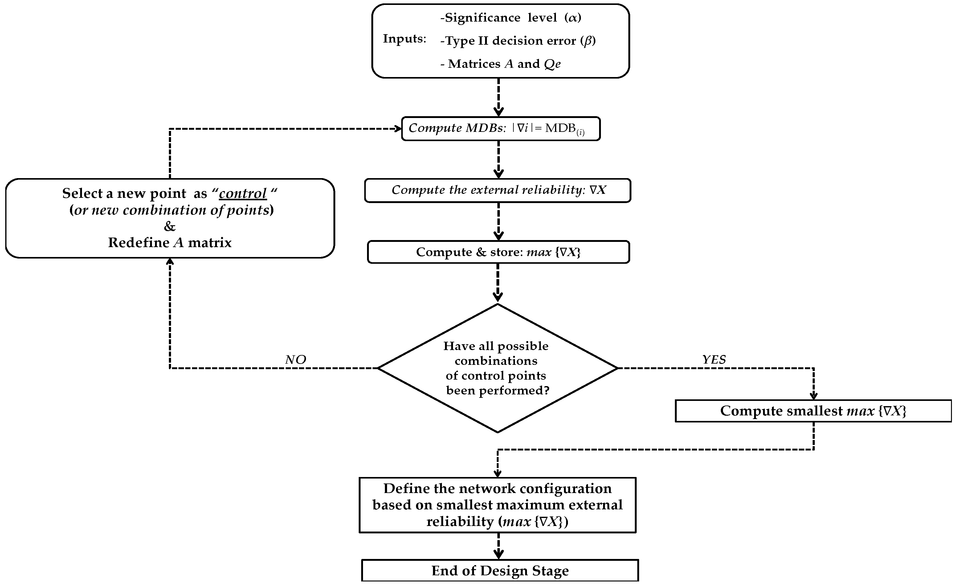
3. Automatic Procedure to Design the Location of Control Points in the Geodetic Network

For the establishment of a geodetic network, we must define which points of the network will have their coordinates previously determined in the desired reference system. These points are called control points, or constraint points. These points that allow the other points of the geodetic network to be linked to a reference system. Therefore, it is essential to define the location of these control points at the design stage of a geodetic network. the proposed automatic method here focuses on designing of the geodetic networks in terms of high reliability. Under the present proposal, the quality criterion to be considered during the design stage is based on the smallest value of the maximum influence of an outlier on the coordinates of the network (i.e., maximum external reliability). The method does not depend on the real measurements values but only on the model design, i.e., the network geometry and covariance matrix. The computations can be performed as follows:

• Defining a significance level $\alpha$ and the type II error $\beta$ in order to compute the non-centrality parameter. Here, we use the recursive algorithm based on the work by Aydin and Demirel [33], namely bisection algorithm, in order to obtain the non-centrality parameter for one degree of freedom, i.e., ${\lambda }_{q=1}$. Typically a value of the level $\alpha =0.001$ and $\beta =0.2$ is adopted (see, e.g., [4]).
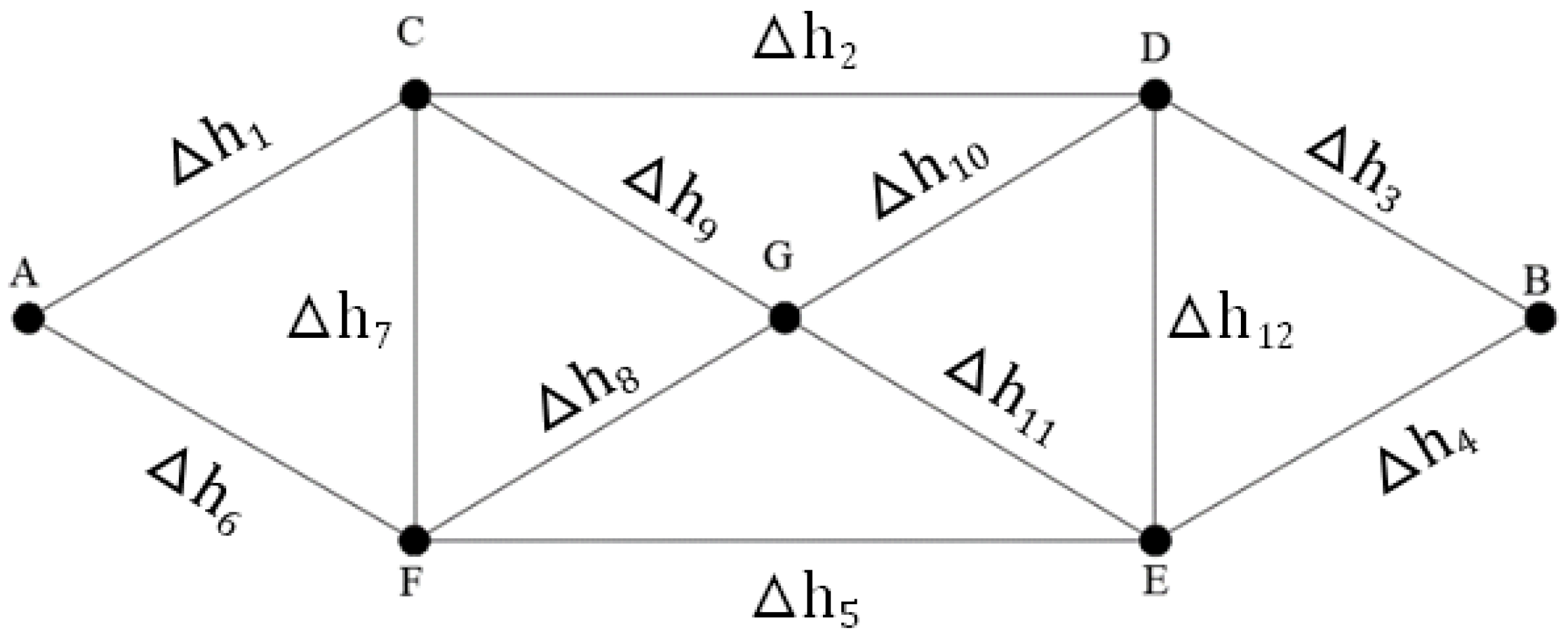
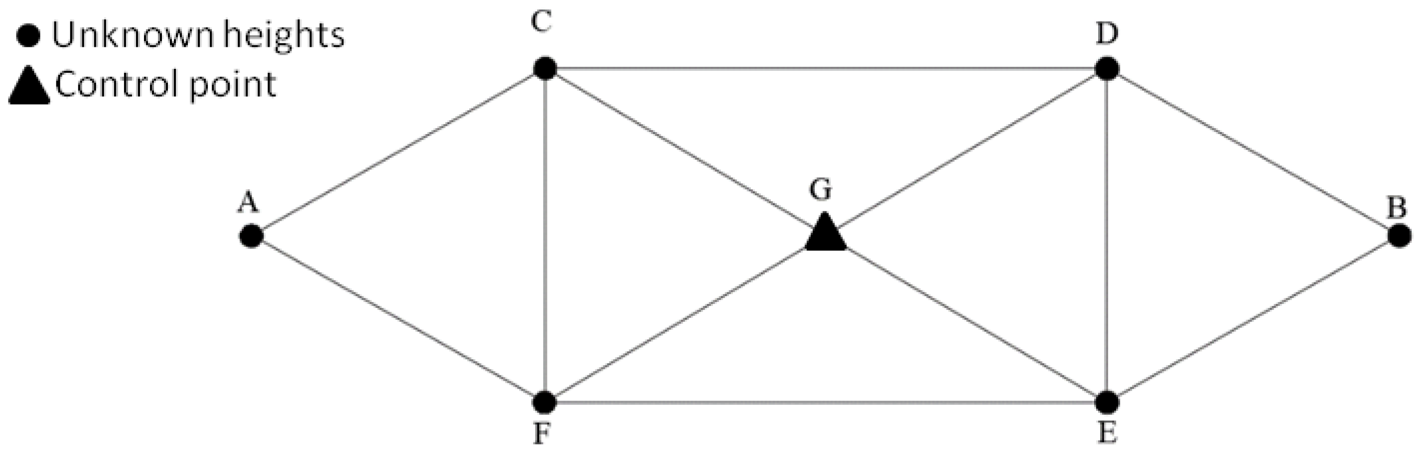
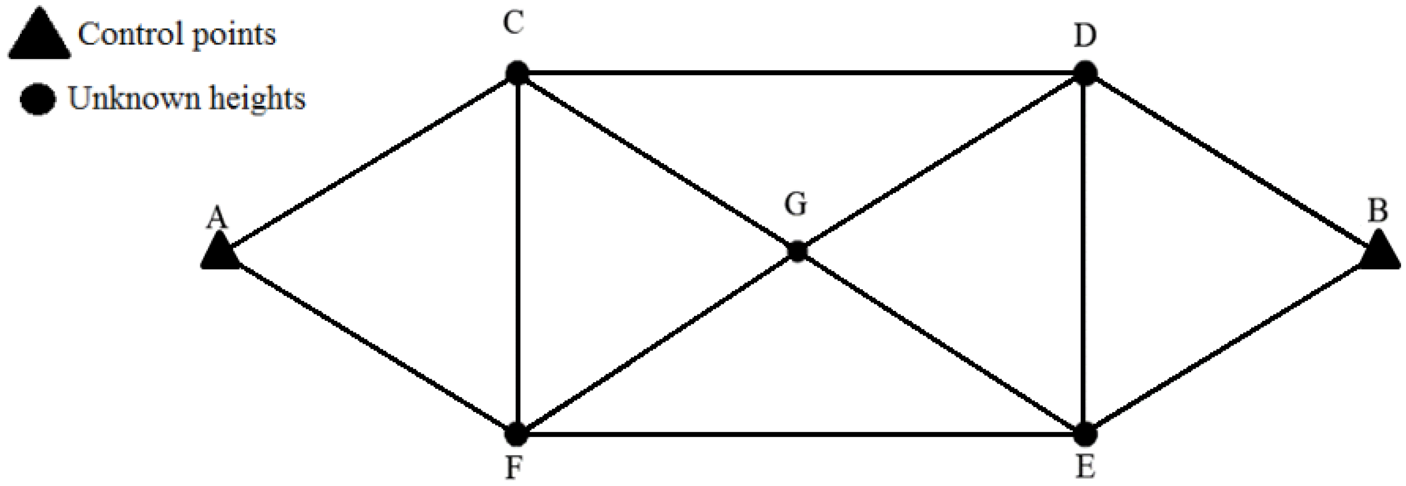
• Defining a geodetic network configuration as well as the uncertainties of the observations, i.e., the design matrix $\mathit{A}$ and the covariance matrix of the observations ${\mathit{Q}}_{\mathit{e}}$, respectively. The covariance matrix of the observations ${\mathit{Q}}_{\mathit{e}}$ may consist of random effects and the uncertainties associated with the correction of systematic effects. The latter follows from the instrument precision, measurement techniques and field condition. In this step, the design matrix and covariance matrix are conditioned to the position of the control point (or by the combination of control points) in the network. It is important to mention that the design matrix defined must have a minimum configuration to avoid rank deficiency [47].
• Computing the MDB for each observation according to Equations (7)–(9).
• Computing the external reliability according to Equation (10).
• Computing and store the maximum external reliability according to Equation (11).
• Checking whether all the points (or all combination of points) of the network were configured as control point. If not, select a new control point (or new combination of control points) and return to Step 3. Otherwise, the algorithm selects the configuration of the network that has the lowest value of the maximum external reliability. Important to mention that matrix $\mathit{A}$ is modified when a new point (or a new combination of points) is selected as the control.

The proposed procedure is summarised as a flowchart in Figure 1.

4. Results and Discussion

In order to demonstrate the design method in practice, in this section we apply it to a closed levelling network. the network is displayed in Figure 2. The goal is to illustrate the design method; further considerations about levelling networks are outside the scope of this study. The results of this paper are presented for $\gamma =0.8$ and $\alpha =0.001$, which gives ${\lambda }_{q=1}=17.075$.

The results of the internal reliability are shown based on the relationship between MDB and the standard-deviation of the observation. As an example of that relationship, for $MDB$ = 5 mm and $\sigma$ = 2.5 mm, the ratio is $\frac{MDB}{\sigma }=\frac{5mm}{2.5mm}=2\Rightarrow MDB=2\sigma$.

Two typical cases were considered here: (a) a minimally constrained and (b) a over-constrained least squares adjustment. The variances of the height difference (denoted by ${\sigma }_{\mathsf{\Delta }{h}_i}^2$) are assumed normally distributed and uncorrelated. The variances were based on the relation between the differential levelling lines and their lengths. In other words, the variances of differential levelling lines are proportional to their lengths, i.e., the larger the lengths, the larger the variances of differential levelling lines.

We consider that the equipment used here is a spirit level with nominal standard deviation of ±1 mm/km for a double run levelling. In each scenario two variants are considered here:

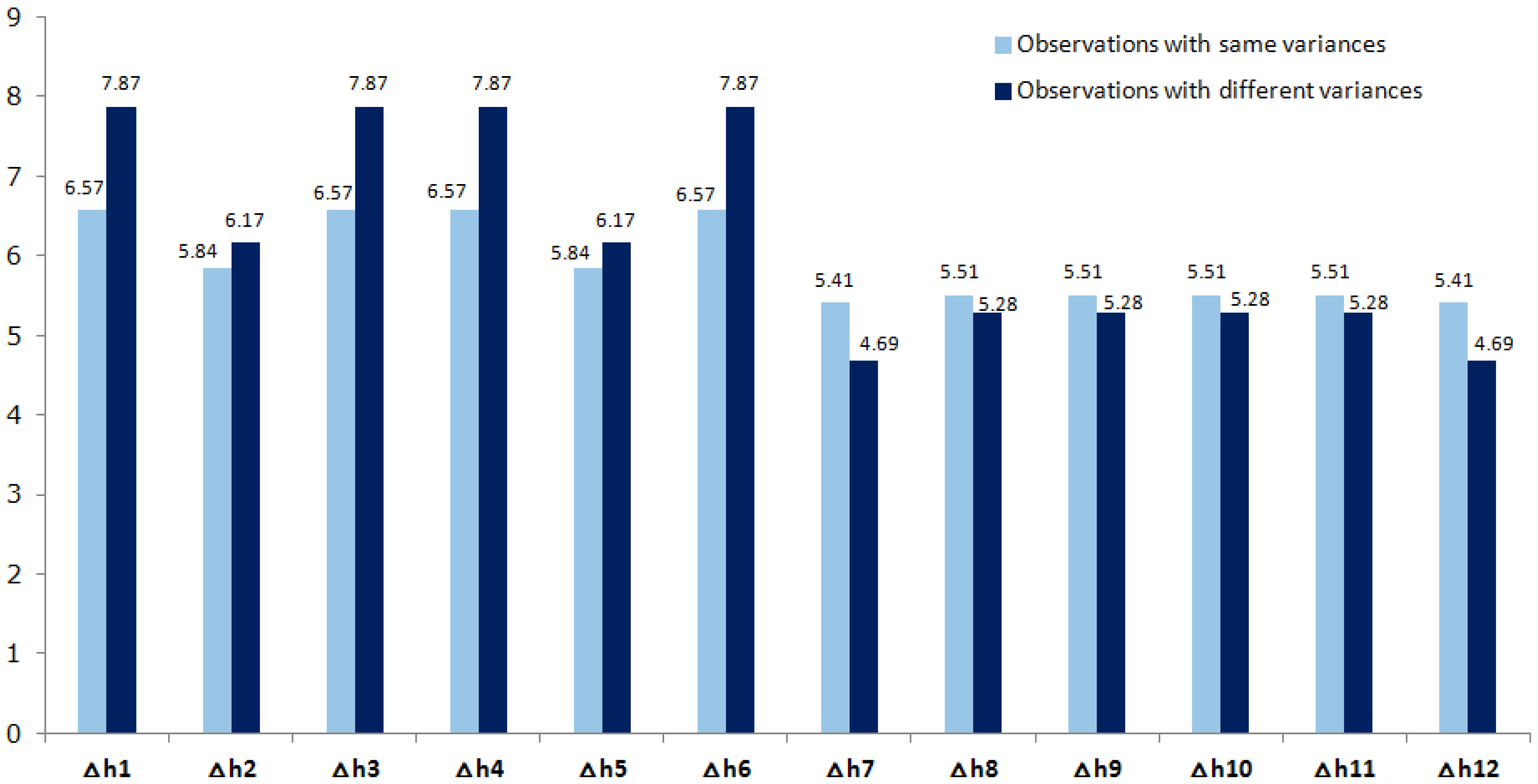
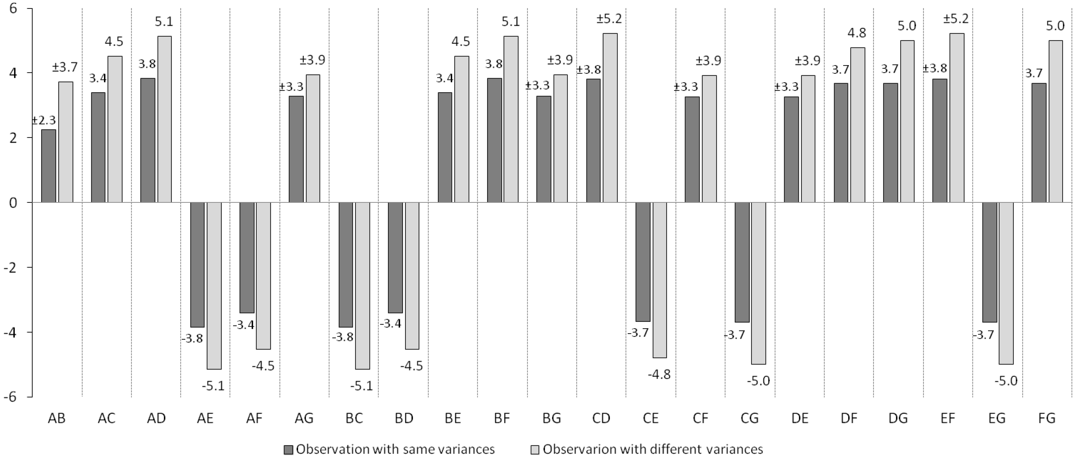
• all lengths of the differential levelling with 1 km, and therefore the variances equal to 1 mm${}^2$; and
• lines with diversified lengths, and therefore levelling lines with different variances, whose values are given in

  Table 1. Levelling lines with different lengths and variances for the Case 2.

  Observation	Length of Line (km)	${\mathit{\sigma }}_{\mathbf{\Delta }{\mathit{h}}_{\mathit{i}}}^{\mathbf{2}}$ (${\mathbf{mm}}^{\mathbf{2}}$)
  ${\mathsf{\Delta }}_{h1}$	1.000	1.00
  ${\mathsf{\Delta }}_{h3}$	1.000	1.00
  ${\mathsf{\Delta }}_{h4}$	1.000	1.00
  ${\mathsf{\Delta }}_{h6}$	1.000	1.00
  ${\mathsf{\Delta }}_{h2}$	1.414	2.00
  ${\mathsf{\Delta }}_{h5}$	1.414	2.00
  ${\mathsf{\Delta }}_{h8}$	1.732	3.00
  ${\mathsf{\Delta }}_{h9}$	1.732	3.00
  ${\mathsf{\Delta }}_{h10}$	1.732	3.00
  ${\mathsf{\Delta }}_{h11}$	1.732	3.00
  ${\mathsf{\Delta }}_{h7}$	2.000	4.00
  ${\mathsf{\Delta }}_{h12}$	2.000	4.00

  .

In the first scenario (a), we consider the closed levelling network in Figure 2 with availability of one control station, and 6 points with unknown heights, totalling six minimally constrained points and 7 possible cases of control point configuration. In that case, there are $n=12$ observations and $u=6$ unknowns, which lead to $n-u=6$ degrees of freedom.

Moreover, the design matrix $\mathit{A}$ has dimension $12\times 6$ and the covariance matrix of observations ${\mathit{Q}}_{\mathit{e}}$ has dimension $12\times 12$. The stations C, D, E, F and G are involved in 4 height differences, so there are three redundant observations for the determination of these heights. On the other hand, there is one redundant observation for the determination of heights of the stations a and B.

The MDBs computed for each observation of the network and for each case of variances configuration are displayed in Figure 3. It is important to mention that MDBs were invariant with regard to the position of a single control point in the network. It can be noted that the observations $\mathsf{\Delta }{h}_7$ and $\mathsf{\Delta }{h}_{12}$ are more resistant to outlier than others, because theirs MDBs were the smallest on the network.

Table 2. Maximum external reliability for a single control point for both observations with equal variances and with different variances.

	Maximum External Reliability (mm)	Maximum External Reliability (mm)
Control Point	Observations with Same Variance	Observations with Different Variances
A	$\pm 3.97$	$\pm 5.70$
B	$\pm 3.97$	$\pm 5.70$
C	$-3.97$	$-5.70$
D	$+3.97$	$+5.70$
E	$-3.97$	$-5.70$
F	$+3.97$	$+5.70$
G	$\pm 3.28$	$\pm 3.94$

shows the maximum external reliability of the network. It can be noted that the smallest value of the maximum influence of an MDB on the heights occurred when the station G was taken as control point, i.e., when the control point was set to the centre of the network (3.28 mm, marked in bold). The ± sign in Table 2 means that the maximum influence of an outlier on the network occurs in two directions (up and down). The best network configuration obtained based on the optimal position of the control point is shown in Figure 4.

In the second case, we consider the closed levelling network in Figure 2 over-constrained with two control stations, totalling 21 possible combinations of control points. For example, taking A and B as fixed, we have $u=5$ unknown heights (C, D, E, F, G), $n=12$ observations and $n-u=7$ redundant observations. In that case, the design matrix $\mathit{A}$ has dimension $12\times 5$ and the covariance matrix of observations ${\mathit{Q}}_{\mathit{e}}$ has dimension $12\times 12$. On the other hand, we have $u=5$ unknown heights (B, D, E, F, G), $n=11$ observations and $n-u=16$ redundant observations in the case of selecting control points a and C. In that case, when the control points are adjacent, the respective levelling line are not observed and, therefore, the design matrix $\mathit{A}$ has dimension $11\times 5$ and the covariance matrix of observations ${\mathit{Q}}_{\mathit{e}}$ has dimension $11\times 11$. Figure 5 shows an example when the control points are adjacent.

For the second case, we produce and analyse 21 graphs showing the MDB values. Due to the large number of graphs, we show here a table with a summary of the results.

Table 3. Statistics of MDB for two control points—over-constrained scenario ($\mathbf{b}$).

	MDB (in $\mathit{\sigma }\mathit{unit}$)
	Observations with Same Variances				Observations with Different Variances
Control Point	Average	Max.	Min.	Sth. Dev.	Average	Max.	Min.	Std. Dev.
AB	5.41	5.41	5.41	0.00	5.52	6.39	4.69	0.67
AC, AF, DB or BE	5.64	6.56	5.1	0.50	5.86	7.83	4.49	1.16
CD or EF	5.69	6.45	4.98	0.63	5.93	7.5	4.6	1.28
CG, DG, EG or FG	5.69	6.56	5.00	0.65	5.97	7.85	4.57	1.35
AD, AE, CB or BF	5.46	6.47	4.99	0.50	5.61	7.43	4.59	1.00
AG or BG	5.48	6.57	4.95	0.57	5.69	7.87	4.57	1.19
DE or CF	5.65	6.53	5.06	0.50	5.8	7.73	4.66	1.03
CE or DF	5.51	6.36	4.90	0.66	5.68	7.16	4.53	1.12

shows the overall statistics of the MDBs (average, maximum, minimum, and standard-deviation) for each possible combination, two by two, of control points and for each scenario of variance. For the case of same variances, it can be noted that when the points A and B were taken as control points (AB), the observations presented a good level of homogeneity (homogeneous redundancy), i.e., all of them had the same internal reliability. It means that, in the presence of an outlier, all observations have the same ability to detect it. This fact is expected and due to the complete symmetry of the network design and the variances of observations. The search for homogeneous redundancy in all the observations has already been investigated in [14,15].

Figure 6 shows the maximum external reliability for the over-constrained network. The maximum external reliability of the network for combinations of control points AB, AG, BG, CD, CF, DE and EF had positive and negative signals. This is represented by the ± sign in Figure 6. It means that the maximum influence of an outlier on the network occurs in two directions. It can be noted that both cases of observations with same variances and different variances, the smallest value of the maximum influence of an MDB on the heights occurred when the stations A and B were fixed as control, with $max(\nabla \mathit{X})=2.3mm$. In general, the inflation of the variances in the network amplified the maximum external reliability, i.e., it increased the maximum influence of a possible outlier on the network. The optimum configuration of the network according to our algorithm is shown in Figure 7.

5. Final Remarks

Within the context of applied sciences, we highlight that the core of the paper is to bring forward a method for automatically selecting the location of the control point (or control points) of geodetic networks based on the reliability theory.

The proposed method to design a geodetic network is based on the smallest value of the maximum external reliability. The size of the outlier is defined according to MDB for a given type I and type II error probabilities. We highlight that the method discards the use of the observation vector of the Gauss–Markov model. In fact, the only needs are the geometrical network configuration (given by Jacobian matrix) and the uncertainties of the observations (given by instrument precision, measurement techniques and/or field condition). Therefore, it can be applied for any kind of geodetic network. In fact, it can be applied to any mathematical modelling for sensitivity analysis. In other words, it can be employed to apportion the changes in outputs of a system to different configuration in its inputs.

The method requires that a priori geodetic network configuration (i.e., geometric configuration and uncertainty of observations) be provided by the user. The user-provided design matrix $\mathit{A}$ presents rank deficiency due to the lack of definition of a network datum. In other words, there are no minimal constraints to solve a rank deficiency of a priori user-provided design matrix $\mathit{A}$. In order to have a matrix $\mathit{A}$ with full rank, the proposed algorithm select a point as control. Next, the maximum external reliability is computed and stored. The procedure is repeated until all network points were selected as a control point. Finally, the algorithm selects the network which has suffered the least influence from a possible undetected outlier. In other words, the algorithm selects that network configuration with the smallest value for maximum external reliability. As shown in the results, the proposed procedure also works for designing geodetic networks with more than one control point.

The proposed method was applied to a closed levelling network. The MDB was computed based on a power of the test of data snooping of 0.80 (80%) and the significance level of 0.001 (0.1%). To apply the concepts in practice, two scenarios were presented for a simulated levelling geodetic network: a minimally constrained network one and a over-constrained network. The observations were assumed normally distributed and uncorrelated, which usually happens in the practice of levelling network adjustment. In each scenario two variants were also considered: one in which the variances of the measurements were assumed equal and another in which the variances were different. In the case of the minimally constrained network, we highlight that the centre of the simulated network was the optimum position to set the control point. In the over-constrained network, we highlight that among the 21 possibilities of configuring the control points, the stations with less line connections (i.e., with less redundant observations) provided the optimum configuration of geodetic network.

This simple example was provided to demonstrate the application of the method. Future experiments based on real data will be performed in order to infer the actual application of the method. The application to more complex networks and others optimization criteria (such as the value and ratio of the eigenvalues of the covariance matrices of the unknowns to predict variances and their homogeneity) will also be investigated in future works.

Furthermore, we highlight that the integration of the reliability and precision as a one-off criterion is an issue in progress for future publications.

References

1. Klein, I.; Matsuoka, M.T.; Guzatto, M.P.; Nievinski, F.G.; Veronez, M.R.; Rofatto, V.F. A new relationship between the quality criteria for geodetic networks. J. Geod. 2019, 93, 529–544. [Google Scholar] [CrossRef]
2. Lehmann, R.; Neitzel, F. Testing the compatibility of constraints for parameters of a geodetic adjustment model. J. Geod. 2013, 87, 555–566. [Google Scholar] [CrossRef] [Green Version]
3. Baarda, W. Statistical concepts in geodesy. Publ. Geod. New Ser. 1967, 2, 74. [Google Scholar]
4. Baarda, W. A testing procedure for use in geodetic networks. Publ. Geod. New Ser. 1968, 2, 5. [Google Scholar]
5. Teunissen, P. Testing Theory: An Introduction, 2nd ed.; Delft University Press: Delft, The Netherlands, 2006. [Google Scholar]
6. Seemkooei, A.A. Comparison of reliability and geometrical strength criteria in geodetic networks. J. Geod. 2001, 75, 227–233. [Google Scholar] [CrossRef]
7. Seemkooei, A.A. Strategy for Designing Geodetic Network with High Reliability and Geometrical Strength. J. Surv. Eng. 2001, 127, 104–117. [Google Scholar] [CrossRef] [Green Version]
8. Lehmann, R. On the formulation of the alternative hypothesis for geodetic outlier detection. J. Geod. 2013, 87, 373–386. [Google Scholar] [CrossRef] [Green Version]
9. Baarda, W. S-transformations and criterion matrices. Publ. Geod. New Ser. 1973, 5, 168. [Google Scholar]
10. Grafarend, E.W. Optimization of Geodetic Networks. Can. Surv. 1974, 28, 716–723. [Google Scholar] [CrossRef]
11. Grafarend, E.W.; Sansò, F. (Eds.). Optimization and Design of Geodetic Networks; Springer: Berlin/Heidelberg, Germany, 1985. [Google Scholar] [CrossRef]
12. Teunissen, P.J.G. Quality Control in Geodetic Networks. In Optimization and Design of Geodetic Networks; Grafarend, E.W., Sansò, F., Eds.; Springer: Berlin/Heidelberg, Germany, 1985; pp. 526–547. [Google Scholar]
13. Vaníček, P.; Craymer, M.R.; Krakiwsky, E.J. Robustness analysis of geodetic horizontal networks. J. Geod. 2001, 75, 199–209. [Google Scholar] [CrossRef]
14. Amiri-Simkooei, A. A new method for second order design of geodetic networks: Aiming at high reliability. Surv. Rev. 2004, 37, 552–560. [Google Scholar] [CrossRef]
15. Amiri-Simkooei, A.; Sharifi, M.A. Approach for Equivalent Accuracy Design of Different Types of Observations. J. Surv. Eng. 2004, 130, 1–5. [Google Scholar] [CrossRef] [Green Version]
16. Hekimoglu, S.; Erenoglu, R.C.; Sanli, D.U.; Erdogan, B. Detecting Configuration Weaknesses in Geodetic Networks. Surv. Rev. 2011, 43, 713–730. [Google Scholar] [CrossRef]
17. Hekimoglu, S.; Erdogan, B. New Median Approach to Define Configuration Weakness of Deformation Networks. J. Surv. Eng. 2012, 138, 101–108. [Google Scholar] [CrossRef]
18. Klein, I.; Matsuoka, M.T.; Souza, S.F.d.; Collischonn, C. Planejamento de redes georesistentes a moutliers. Boletim CiGeod. 2012, 18, 480–507. [Google Scholar]
19. Rofatto, V.; Matsuoka, M.; Klein, I. Design of geodetic networks based on outlier identification criteria: An example applied to the leveling network. Bull. Geod. Sci. 2018, 24, 152–170. [Google Scholar] [CrossRef]
20. Knight, N.L.; Wang, J.; Rizos, C. Generalised measures of reliability for multiple outliers. J. Geod. 2010, 84, 625–635. [Google Scholar] [CrossRef]
21. Imparato, D.; Teunissen, P.; Tiberius, C. Minimal Detectable and Identifiable Biases for quality control. Surv. Rev. 2019, 51, 289–299. [Google Scholar] [CrossRef]
22. Rofatto, V.F.; Matsuoka, M.T.; Klein, I.; Veronez, M.R.; Bonimani, M.L.; Lehmann, R. A half-century of Baarda’s concept of reliability: A review, new perspectives, and applications. Surv. Rev. 2018, 0, 1–17. [Google Scholar] [CrossRef]
23. Rofatto, V.F.; Matsuoka, M.T.; Klein, I.; Veronez, M.R. Monte-Carlo-based uncertainty propagation in the context of Gauss–Markov model: A case study in coordinate transformation. Sci. Plena 2019, 15, 1–17. [Google Scholar] [CrossRef]
24. Koch, K.R. Parameter Estimation and Hypothesis Testing in Linear Models, 2nd ed.; Springer: Berlin, Germany, 1999. [Google Scholar]
25. Ghilani, C.D. Adjustment Computations: Spatial Data Analysis, 6th ed.; John Wiley & Sons, Ltd.: Hoboken, NJ, USA, 2017. [Google Scholar]
26. Lehmann, R. Improved critical values for extreme normalized and studentized residuals in Gauss–Markov models. J. Geod. 2012, 86, 1137–1146. [Google Scholar] [CrossRef]
27. Kargoll, B. On the Theory and Application of Model Misspecification Tests in Geodesy. Ph.D. Thesis, University of Bonn, Bonn, Germany, 2007. [Google Scholar]
28. Yang, L.; Wang, J.; Knight, N.L.; Shen, Y. Outlier separability analysis with a multiple alternative hypotheses test. J. Geod. 2013, 87, 591–604. [Google Scholar] [CrossRef]
29. Teunissen, P. Distributional theory for the DIa method. J. Geod. 2018, 92, 59–80. [Google Scholar] [CrossRef]
30. Teunissen, P. An Integrity and Quality Control Procedure for use in Multi Sensor Integration. In ION GPS Redbook Volume VII Integrated Systems; Institute of Navigation (ION): Manassas, VA, USA, 1990. [Google Scholar]
31. Vaníček, P.; Krakiwsky, E.J. Geodesy: The Concepts, 2nd ed.; Elsevier Science: Amsterdam, The Netherlands, 1987. [Google Scholar]
32. Lehmann, R. Observation error model selection by information criteria vs. normality testing. Stud. Geophys. Geod. 2015, 59, 489–504. [Google Scholar] [CrossRef] [Green Version]
33. Aydin, C.; Demirel, H. Computation of Baarda’s lower bound of the non-centrality parameter. J. Geod. 2004, 78, 437–441. [Google Scholar] [CrossRef]
34. Wang, J.; Chen, Y. On the reliability measure of observations. Acta Geod. Cartogr. Sin. 1994, 4, 42–51. [Google Scholar]
35. Pelzer, H. Detection of errors in the functional adjustment model. In Mathematical Models of Geodetic/Photogrammetric Point Determination with Regard to Outliers and Systematic Errors; Ackermann, F., Ed.; German Geodetic Commission: Munich, Germany, 1983. [Google Scholar]
36. Prószyński, W. Criteria for internal reliability of linear least squares models. Bull. GÉOdÉSique 1994, 68, 162–167. [Google Scholar] [CrossRef]
37. Schaffrin, B. Reliability Measures for Correlated Observations. J. Surv. Eng. 1997, 123, 126–137. [Google Scholar] [CrossRef]
38. Teunissen, P.J.G. Minimal detectable biases of GPS data. J. Geod. 1998, 72, 236–244. [Google Scholar] [CrossRef] [Green Version]
39. Prószyński, W. Another approach to reliability measures for systems with correlated observations. J. Geod. 2010, 84, 547–556. [Google Scholar] [CrossRef] [Green Version]
40. Ding, X.; Coleman, R. Multiple outlier detection by evaluating redundancy contributions of observations. J. Geod. 1996, 70, 489–498. [Google Scholar] [CrossRef]
41. Gui, Q.; Li, X.; Gong, Y.; Li, B.; Li, G. a Bayesian unmasking method for locating multiple gross errors based on posterior probabilities of classification variables. J. Geod. 2011, 85, 191–203. [Google Scholar] [CrossRef]
42. Gökalp, E.; Güngör, O.; Boz, Y. Evaluation of Different Outlier Detection Methods for GPS Networks. Sensors 2008, 8, 7344–7358. [Google Scholar] [CrossRef] [PubMed]
43. Baselga, S. Nonexistence of Rigorous Tests for Multiple Outlier Detection in Least-Squares Adjustment. J. Surv. Eng. 2011, 137, 109–112. [Google Scholar] [CrossRef]
44. Klein, I.; Matsuoka, M.T.; Guzatto, M.P.; Nievinski, F.G. An approach to identify multiple outliers based on sequential likelihood ratio tests. Surv. Rev. 2017, 49, 449–457. [Google Scholar] [CrossRef]
45. Lehmann, R.; Lösler, M. Multiple Outlier Detection: Hypothesis Tests versus Model Selection by Information Criteria. J. Surv. Eng. 2016, 142, 04016017. [Google Scholar] [CrossRef] [Green Version]
46. Fu, L.; Zhang, J.; Li, R.; Cao, X.; Wang, J. Vision-Aided RAIM: A New Method for GPS Integrity Monitoring in Approach and Landing Phase. Sensors 2015, 15, 22854–22873. [Google Scholar] [CrossRef] [Green Version]
47. Xu, P. Sign-constrained robust least squares, subjective breakdown point and the effect of weights of observations on robustness. J. Geod. 2005, 79, 146–159. [Google Scholar] [CrossRef] [Green Version]
Figure 1. Flowchart of the automatic method proposed to design the location of control points in the geodetic network.
Applsci 10 00687 g001
Figure 2. Simulated levelling geodetic network.
Applsci 10 00687 g002
Figure 3. MDB ( σ ) for a single control point—minimally constrained scenario (a)—for the cases of observations with same variances and different variances.
Applsci 10 00687 g003
Figure 4. Optimum Configuration of the network for a single control point—minimally constrained scenario (a).
Applsci 10 00687 g004
Figure 5. Example of the network configuration for adjacent control points a and C.
Applsci 10 00687 g005
Figure 6. Maximum external reliability max ( X ) [mm] for two control points in the network.
Applsci 10 00687 g006
Figure 7. Optimum configuration of the network for two control points.
Applsci 10 00687 g007