Application of Metal Magnetic Memory Testing Technology to the Detection of Stress Corrosion Defect


1
Department of Mechanics, School of Civil Engineering, Beijing Jiaotong University, Beijing 100044, China
2
Department of Mechanics, School of Mechanical Engineering, Tianjin University, Tianjin 130350, China
*
Authors to whom correspondence should be addressed.
Appl. Sci. 2020, 10(20), 7083; https://doi.org/10.3390/app10207083
Submission received: 22 September 2020
/
Revised: 7 October 2020
/
Accepted: 10 October 2020
/
Published: 12 October 2020
(This article belongs to the Special Issue Nondestructive Testing (NDT): Volume II)
Abstract
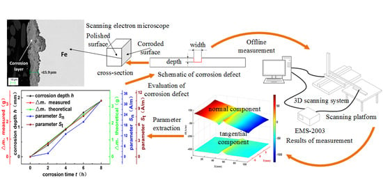
:The damage of equipment manufactured with ferromagnetic materials in service can be effectively detected by Metal Magnetic Memory Testing (MMMT) technology, which has received extensive attention in various industry fields. The effect of stress or strain on Magnetic Flux Leakage (MFL) signals of ferromagnetic materials has been researched by many scholars for assessing stress concentration and fatigue damage. However, there is still a lack of research on the detection of stress corrosion damage of ferromagnetic materials by MMMT technology. In this paper, the electrochemical corrosion system was designed for corrosion experiments, and three different experiments were performed to study the effect of corrosion on MFL signals. The distribution of MFL signals on the surface of the specimen was investigated. The results indicated that both the normal component Hn and tangential component Ht of MFL signals presented different signal characteristics when the specimen was subjected to different working conditions. Finally, two characterization parameters, Sn and St, were defined to evaluate the corrosion degree of the specimen, and St is better. The direct dependence of corrosion depth on the parameter was developed and the average error rates between the predicted and measured values are 8.94% under the same working condition. Therefore, the expression can be used to evaluate the corrosion degree of the specimen quantitatively. The results are significant for detecting and assessing the corrosion defect of ferromagnetic materials.
1. Introduction
Many types of equipment manufactured with ferromagnetic materials in service are working under the condition of stress corrosion. Most of this equipment is susceptible to corrosion defects. The effect of pitting corrosion on pipeline steel has been studied by many scholars [1,2,3,4]. Chen and Zhao reported the failure of oil and gas pipelines due to stress corrosion cracking [5,6]. It is necessary to conduct Non-Destructive Testing (NDT) for stress corrosion defects. The common NDT method for the quantitative evaluation of corroded defects, such as Electrochemical Noise Analysis (ENA), has been studied by many scholars [7,8,9]. It was used to investigate the corrosion behavior of mild steel (Q235) [10], and Wang reported that pitting corrosion of high strength steel is quantitatively evaluated by combining 3-D measurement and image-recognition-based statistical analysis [11]. However, the reliability for assessing the sizes of corrosion defects needs to be further discussed. The traditional magnetic testing technologies [12,13,14], such as magnetic particle testing [15,16], magnetic flux leakage testing [17,18,19], usually require a large external magnetic field [20,21,22], which is inconvenient to operate and even impractical under some conditions. Although the non-destructive testing of stress corrosion defects has been widely studied, the traditional NDT methods have some limitations. Therefore, it is necessary to develop a more simple and effective NDT technology.
The Metal Magnetic Memory Testing (MMMT) technology, which was first presented at the 50th International Welding Conference in 1997 by a Russian researcher, is an emerging testing method in the field of non-destructive testing technology [23,24]. It is a weak-field detecting method, which uses the geomagnetic field instead of an artificial magnetic field as the stimulus source. MMMT technology is used to diagnose the early damage by measuring the self-magnetized leakage field on the surface of ferromagnetic materials [25,26]. MMMT technology has the advantages of simple equipment, simple operation, and no treatment on the surface of the tested part. Nowadays, the MMMT technique has attracted the attention of scholars in many industry fields, such as machinery, pressure vessels, pipelines, etc. [27,28]. It is widely studied by many scholars for its advantages over other magnetic testing methods [29,30,31], and the stress–magnetism effect has also been widely studied [32,33,34]. The impact of stress or strain on Magnetic Flux Leakage (MFL) signals of ferromagnetic materials has been researched for assessing stress concentration [35,36] and fatigue damage [37,38,39]. The previous study [40] showed that the ambient stress conditions during corrosion defect formation would affect the MFL signals based on magnetic flux leakage testing. In recent years, MMMT was applied to the detection of rebar corrosion in concrete and the commonly used steel strand in structural engineering to locate the corrosion area and evaluated the corrosion degree [41,42]. However, there is still a lack of research on stress corrosion. Therefore, it is very promising to detect stress corrosion defects by MMMT technology.
In this paper, three experiments were performed to study the effect of corrosion on magnetic leakage signals. The electrochemical corrosion system was designed for corrosion experiments. The distribution regularity of MFL signals during the corrosion process was investigated. The feasibility of evaluating the degree of corrosion of ferromagnetic materials using the MFL signals was discussed.
2. Experimental Section
To study the effect of corrosion on MFL signals, three different experiments were performed. Experiment 1 is a static tensile experiment; experiment 2 and experiment 3 are corrosion experiments: Experiment 2 is a corrosion experiment without loading; experiment 3 is a corrosion experiment after loading. In addition, the Scanning Electron Microscope (SEM) and Energy Dispersive X-Ray Spectroscopy (EDX) were used to observe the surface of the specimen and analyze the corrosion layer, respectively.
2.1. Specimen Preparation
The specimens were made by 0.45% C steel in this study, which is medium-carbon structural steel and widely used in the structural engineering field. Composition of 0.45% C steel, % by weight is C (0.42–0.50%), Si (0.17–0.37%), Mn (0.50–0.80%), P (≤0.035%), S (≤0.035%). Its mechanical properties are listed in Table 1. Flat dog-bone specimens designed based on GB/T228-2002 were prepared without (used in corrosion experiments) and with a groove (used in the static tensile experiment). The rectangular groove (6.8 mm width and 2 mm depth) was carefully made by a linear cutting machine in the middle of the specimens. The specimen was designed to be a special shape (dog bone) to obtain a uniform distribution of stress in the corrosion area.
The shape and size of the 6-mm-thick specimens used in the experiments were drawn in Figure 1. Five scanning lines with a length of 100 mm, denoted as Line 1, Line 2, Line 3, Line 4, and Line 5, were parallel to each other at intervals of 4.5 mm. Line 3 is the centerline of the specimen.
Before experiments, all of the specimens were polished to grade P1000 grit, followed by rinsing with isopropyl alcohol, drying in warm air, and weighing with an electronic balance. The specimen was polished only to remove the corrosion on the specimen surface and measure the mass loss of the specimen more accurately. In addition, every specimen was demagnetized before it was loaded or corroded to eliminate the effect of mechanical processing on the magnetic field.
2.2. Description of Corrosion and Detection System
The schematic of the set-up for the corrosion system is shown in Figure 2a. The electrochemical method was used to accelerate the corrosion of the specimen. The working electrode is the specimen connected to the positive electrode of the direct current (DC) power source (UTP3303, produced by UNI-TREND Technology (China) CO. LTD). The copper sheet was served as a counter electrode connected to the negative electrode of the DC power source. There is no direct contact between the electrolyte and the specimen. The electrolyte contacts the surface of the specimen placed on a plastic block above the electrolyte level through a specially shaped sponge (Corrosion area = 175 mm2). The electrolyte for the corrosion process was 3.5% (wt.%) NaCl solution. In corrosion experiments, the specimen is corroded by galvanostatic corrosion of 0.4 A.
Two Faraday’s laws of electrolysis govern the mass of anodic material corroded or consumed when the current passes through the circuit.
Hence, the mass of substance (△m, theoretical):
where K is electrochemical equivalent; n is the valence of the substance; M is the atomic mass or the molecular weight of the substance; F is Faraday’s constant, 96,494 C/mole; I is the current in the electrochemical reaction; t is time in hours.
The corrosion experiments were divided into four stages: Accelerated corrosion was performed by the galvanostatic corrosion method using 0.4 A current for 2 h in the first corrosion stage, and the corrosion products of specimens were rinsed off carefully. Then the specimens were dried in warm air and weighed with an electronic balance to calculate the mass loss △m. The geometric dimensions (width and depth) of corrosion defects at every scanning line of specimens were measured to calculate the average value of them. After that, the specimens were corroded again for 2 h and repeated the above procedure until the specimens were corroded for 8 h.
Corrosion at different stages are given in Table 2. Photographs of the corroded specimen, at various corrosion stages during the experiment, and the schematic of corrosion defect are shown in Figure 3. Variations of mass loss of the specimen (△m, measured and △m, theoretical) and defect feature (depth h) with corrosion time (t) are shown in Figure 4. It is found that the defect depth is associated with mass loss (△m, measured). With the increase of corrosion time, the defect depth and mass loss (measured and theoretical) have the same variation tendency.
The three-dimensional (3D) MFL detection system involves three main parts: a 3D scanning console system, a commercial EMS2003 metal magnetic memory testing apparatus, and a non-magnetic scanning platform. A Hall probe with a resolution of 1 A/m is a part of the testing apparatus, which was fixed on a non-magnetic 3D scanning console system controlled by a computer moving automatically at a uniform detection speed (90 mm/min). The specimens were placed on the scanning platform along the south-north direction when the MFL signals were detected. The data were stored in the EMS2003 metal magnetic memory testing apparatus. The schematic of the 3D MFL detection system is shown in Figure 2b.
2.3. Testing Method
2.3.1. Static Tension Experiment
The tensile tests were performed with a universal testing machine named SANS-100kN, whose load error is within ±0.5%. Before loading, all specimens were demagnetized and put on the platform along the south-north direction to eliminate the influence of the sample orientation. The normal and tangential components of the demagnetization signals, namely Hn and Ht signals, were measured along the south-north direction using the 3D MFL detection system under the condition of room temperature. Tensile loads were applied at an increment of 5 kN. The specimens were measured offline to eliminate any possible effect of the machine, and the MFL signals of specimens were measured in the same way as the demagnetization signals. Then the specimens were loaded to a specific value, and the procedure was repeated until the specimen was loaded to 25 kN.
2.3.2. Corrosion Experiment without Loading
The experiment was divided into four stages. Before the experiment, the specimens were demagnetized and put on the platform along the south-north direction. The demagnetization signals of each scanning line were measured in the same way as the static tension experiment. Then the specimens were corroded for 2 h, and the corrosion products were rinsed off carefully. The specimens were dried in warm air and weighed. The geometric dimensions (width and depth) of corrosion defects were measured, and the MFL signals of every scanning line were measured in the same way as the demagnetization signals. After that, the specimens were corroded again for 2 h, and the procedures were repeated until the specimens were corroded for 8 h.
2.3.3. Corrosion Experiment after Loading
The measurement obtained yield stress of 50 kN for material before the experiment, so the specimens were loaded to a pre-determined value 25 kN. Before the experiment, the specimens were demagnetized and put on the platform along the south-north direction. The demagnetization signals of each scanning line were measured in the same way as the static tension experiment before load. Then the specimens were loaded on the machine, and the MFL signals of every scanning line were measured offline in the same way as the demagnetization signals. After that, the specimens were corroded in the same way as experiment 2 (corrosion without loading).
2.3.4. Surface Characterization
A sample was prepared for SEM to observe the surface of the uncorroded sample. The dimensions of this sample after being cut were 10 × 5 × 3 mm. The surface of the sample was wet ground through successive grades of SiC papers from P180 to P2000 and then polished until there were no scratches. Finally, the sample was immersed in etching reagent, 4mL HNO3 + 96 mL ethanol, for 5–10 s. The surface of the specimen was observed by LEO-1450 SEM equipped with KEVEX-Superdry EDX.
After the corrosion experiment, the dimensions of corrosion sections being cut were 10 × 5 × 3 mm to observe the surface of the sample by SEM. In addition, the cross-section of the sample was found to analyze the thickness and composition of the corrosion layer. To prevent the corrosion layer on the surface of the sample from being damaged artificially during grinding and polishing, the sample was cast into epoxy resin. Then the cross-section of the sample was wet ground and polished by the above treatment method. SEM and EDX observed the cross-section of the sample.
3. Results and Discussion
It should be noted that three specimens in each experiment (experiment 1, 2 and 3) were tested. MFL signals on all testing lines are the same. Thus, the MFL signals on Line 3 are shown here.
3.1. Experimental Results
The distributions of MFL signals (Hn and Ht) during experiment 1 (static tension) under different loads were plotted in Figure 5. It is found that the normal component Hn and the tangential component Ht presented different signal characteristics at the defect during the load process from Figure 5. As can be seen in Figure 5, the demagnetization signals at the defect presented prominent distortion characteristics. Hn presented a “trough-peak” shape, while Ht presented a “peak” shape. Compared with the demagnetization signals, the MFL signals at the defect occurred significant changes after loading. The normal component Hn changed from “trough-peak” to “peak-trough,” while the tangential component Ht changed from “peak” to “trough”; and the baseline amplitude value of Hn and Ht besides the defect increased dramatically. In addition, with the increase of the applied load, the abnormal peak amplitude of Hn and Ht increased. The theory of the magnetic charge can explain the change of MFL signals during the load process [39,41].
The distributions of MFL signals (Hn and Ht) during experiment 2 (corrosion without loading) at different corrosion degrees were plotted in Figure 6. It is found that Hn and Ht of the demagnetization signal presented other characteristics. Hn showed an approximately linear change along Line 3 with a shallow gradient, while Ht kept a nearly constant value. As can be seen in Figure 6, Hn and Ht presented different distortion characteristics at the defect during the corrosion process. Hn presented a “trough-peak” shape, while Ht presented an apparent “peak” shape. With the increase of corrosion degree, the abnormal peak amplitude of Hn and Ht increased. The results indicated that both Hn and Ht presented abnormal peak features during the corrosion process, showing the location of corrosion defect accurately.
The distributions of MFL signals (Hn and Ht) during experiment 3 (corrosion after loading) at different corrosion degrees were plotted in Figure 7. It is found that Hn and Ht of the demagnetization signal also presented different characteristics. Hn showed an approximately linear change along Line 3 with a shallow gradient, while Ht kept an almost constant value. After the specimen was loaded, the gradient and amplitude of Hn increased significantly, while changes only in amplitude could be found for Ht, still almost horizontal linear distribution. Such a phenomenon is due to the piezomagnetic effect [43]. It is known that applied stress can lead to the reorientation of magnetic domains along the tensile direction [44]. As can be seen in Figure 7, Hn and Ht presented different distortion characteristics at the defect during the corrosion process. Hn presented a visible “trough-peak” shape, while Ht presented an apparent “peak” shape. With the increase of corrosion degree, the abnormal peak amplitude of Hn and Ht increased significantly. At the same time, the gradient of Hn and the baseline amplitude value of Hn and Ht decreased. The results of experiment 3 (corrosion after loading) indicated that both Hn and Ht presented abnormal signal characteristics during the corrosion process, showing the location of the corrosion defect accurately.
3.2. Comparison of Experimental Results
The normal components Hn and the tangential component Ht of MFL signals in the last stage in three experiments were selected to compare the characteristics of signals under different working conditions. The surface and contour maps of signals in the chosen stage were drawn in Figure 8. As can be seen in Figure 8a, Hn and Ht of experiment 1 at the defect showed apparent “peak-trough” shape and “trough” shape, respectively. As can be seen in Figure 8b,c, Hn and Ht at the defect presented a “trough-peak” shape, and “peak” shape, respectively. Figure 9a shows the comparison of unprocessed Hn in three experiments. For the convenience of comparison, Hn and Ht were further processed. Hn subtracts the baseline amplitude, and the baseline amplitude of Ht returns to zero. Figure 9b shows the comparison of Hn subtracting the baseline amplitude value in three experiments. Figure 9c shows the comparison of Ht where the baseline amplitude returns to zero in three experiments. It is found that Hn and Ht presented different signal characteristics under different working conditions: When the specimen was subjected to tensile load and corrosion, respectively, Hn and Ht both exhibited opposite signal characteristics. When the specimen was corroded without and after loading, Hn and Ht both showed the same signal characteristics, and a more substantial amplitude value could be found in corrosion experiment after loading.
3.3. Characterization of the Corrosion Layer
The SEM micrographs of the surface of the samples are shown in Figure 10. As can be seen in Figure 10a, the microstructure of the uncorroded sample was composed of lamellar pearlite and white ferrite. As can be seen in Figure 10b, the surface of the sample was covered with relatively uniform corrosion products after 8 h of corrosion. Figure 11 shows the cross-section SEM image, analytical line, and corresponding X-ray maps of Fe and O for the sample corroded for 8 h. The thickness of the corrosion layer is relatively uniform, approximately 16 μm. As can be seen in X-ray maps, the corrosion layer mainly contained oxygen and iron elements. Compared with the iron matrix, the content of the oxygen element in the corrosion layer increased obviously. In contrast, the content of iron decreased obviously, indicating that the corrosion layer was mainly constituted of iron oxides. Therefore, the permeability of the corrosion layer is much less than iron [45], and the corrosion layer reduced the permeability of the sample.
3.4. Analysis and Discussion
The magnetic charge is an equivalent model, which has been developed to interpret the magnetic field leakage of ferromagnetic materials. For a ferromagnet, its external magnetic field would be considered to originate from the magnetic charge [41]. For the convenience of discussion, it is assumed that the magnetic flux leakage was caused by the equivalent magnetic charge on the two interfaces of the defect zone. Then, the MFL H at the measuring point caused by equivalent magnetic charge q is given as
where is the permeability of air, r is the position vector from equivalent magnetic charge to measuring point.
The schematic diagram of MFL signals in experiment 1 (static tensile) is shown in Figure 12a. The initial leakage magnetic field Hi is formed by the magnetic polarity generated due to the accumulation of a small number of magnetic charges at both sides of the defect after the specimen was demagnetized [39,41,46], which coincides with the initial magnetic field He. The demagnetization signals are the vector sum of He and Hi. Thus, Hn presents a “trough-peak” shape, and Ht gives a “peak” shape at the defect. After being loaded, the magnetization of the specimen changes under the combined action of the geomagnetic field and stress [43,44], results in the formation of leakage magnetic field HL. The accumulation of more magnetic charges at both sides of the defect due to the stress concentration at the defect after the specimen was loaded, resulting in a strong leakage magnetic field Hm, which is opposite to the leakage magnetic field Hi. In addition, the leakage magnetic field Hm is stronger than Hi, causing the reversal of MFL signals at the defect. Under such conditions, the MFL signals are the vector sum of the initial magnetic field He, leakage magnetic field HL, Hm, and Hi. Thus, the normal component Hn of MFL signals at the defect presents a “peak-trough” shape, and the tangential component Ht shows a “trough” shape. With the increase of the load, the stress concentration on both sides of the defect increases, increasing the number of magnetic charges, which leads to the strengthening of leakage magnetic field Hm, causing the increase of the MFL signals at the defect (see Figure 5).
The schematic diagram of MFL signals in experiment 2 (corrosion without loading) is shown in Figure 12b. The defect formed on the surface of the specimen due to corrosion, results in the formation of an initial leakage magnetic field Hi. In addition, magnetic charges accumulated at both sides of the defect due to the effect of corrosion, result in the formation of leakage magnetic field Hc, which is opposite to the initial magnetic field Hi. Under such conditions, the MFL signals are the vector sum of the initial magnetic field He, leakage magnetic field Hc and Hi. Thus, the normal component Hn of MFL signals presents a “trough-peak” shape, and the tangential component Ht presents a “peak” shape. With the increase of corrosion degree, the leakage magnetic field Hc is gradually enhanced, causing the MFL signals increasing at the defect (see Figure 6).
The schematic diagram of MFL signals in experiment 3 (corrosion after loading) is shown in Figure 12c. Different from experiment 2, the specimen in experiment 3 was corroded after having been loaded, so a strong leakage magnetic field Hc was generated at the defect after the specimen was corroded, which is stronger than the leakage magnetic field Hm and Hi. Under such conditions, the MFL signals are the vector sum of the initial magnetic field He, leakage magnetic field HL, Hc, Hm, and Hi. Thus, the normal component Hn of MFL signals presents a “trough-peak” shape, and the tangential component Ht presents a “peak” shape. With the increase of corrosion degree, the vector sum of leakage magnetic field Hc, Hm, and Hi increases, causing the MFL signals at the defect gradually increasing (see Figure 7).
4. Quantitative Evaluation Parameters
To further analyze the relationship between the MFL signals and corrosion degree, two characteristic magnetic parameters Sn and St were defined. The parameters Sn and St were extracted from the MFL signals of representative scanning line (Line 3) in experiment 3 (corrosion after loading), and the calculation methods of magnetic characteristic parameters are shown in Figure 13. For the normal component presented in Figure 13a, the parameter Sn can be obtained directly. The parameter Sn is calculated by taking the signal difference between the peak and trough of the Hn. However, the tangential component Ht presented in Figure 13b and the parameter St cannot be obtained straightforwardly. Figure 13c shows the gradient of Ht, the position of the peak and trough of the gradient, A and B, can be obtained directly. Therefore, the parameter St can be calculated by taking the distance from the peak position of Ht to line AB.
Variations of characteristic magnetic parameters (Sn and St), mass loss of the specimen (△m, measured and △m, theoretical), and defect feature (corrosion depth h) with corrosion time (t) are shown in Figure 14. It is found that magnetic characteristic parameters, mass loss, and corrosion depth have the same variation tendency. St is considered to be the best parameter for quantitatively evaluating the degree of the corrosion among the four characterization parameters.
The relationship between the parameter St and the corrosion time t is shown in Figure 15. It is found that the parameter St and the corrosion time t have established a good linear relationship. After linear fitting, the equation defining the dependence of St on t was found, and the correlation coefficient R2 = 0.999:
The direct dependence of mass loss (△m, theoretical) on the parameter St was obtained by Equations (3) and (5) as follows:
At the same time, the width change of the corrosion defect is small in the corrosion test, so the area of the corrosion area S is considered unchanged. The corrosion depth h, theoretical can be calculated from the mass loss △m, theoretical:
where is the density of the specimen. The direct dependence of corrosion depth (h, theoretical) on the parameter St, , was obtained by Equations (6) and (7) as follows:
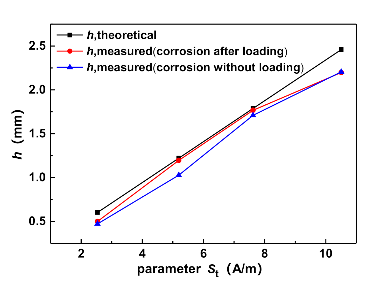
In order to verify the reliability of the expression, the comparison between corrosion depth h, theoretical obtained by parameter St and h, measured in experiment 3 (corrosion after loading) is shown in Figure 16. Meanwhile, corrosion depth h, measured in experiment 2 (corrosion without loading), is also shown in Figure 16. The average error rates of experiment 2 and experiment 3 were calculated to be 15.65% and 8.94%, respectively. It is found that the expression can predict the corrosion depth well and has a smaller error under the same working condition.
5. Conclusions
In this paper, static tensile experiments, corrosion experiments without and after loading were performed to study the effect of corrosion on MFL signals. The normal and tangential components of the MFL signals, namely Hn and Ht, were measured using the 3D MFL detection system, and the distribution regularity of them during the corrosion process was investigated. The following conclusions are obtained:
- (1)
- The normal and tangential components of the MFL signals in corrosion experiments without and after loading presented a “trough-peak”, and “peak” shape, respectively. It is known from experimental results that when the specimen was corroded without and after loading, the normal and tangential components both showed the same signal characteristics, and a more substantial amplitude value could be found in the corrosion experiment after loading.
- (2)
- The normal and tangential components of the MFL signals in the static tensile experiment presented a “peak-trough”, and “trough” shape, respectively. It is found that the normal and tangential components showed different signal characteristics under different working conditions: When the specimen was subjected to tensile load and corroded, respectively, the normal and tangential components both exhibited opposite signal characteristics. According to the analysis, the critical reason for different signal characteristics is that the leakage magnetic field Hc generated at the defect after the specimen has been corroded is opposite to the leakage magnetic field Hm caused by force.
- (3)
- The characterization parameters of MFL signals, Sn and St, are capable of evaluating the corrosion degree of the specimen, and St is better. The characterization parameter of the tangential component of the MFL signals is more sensitive to the corrosion, which is different from the traditional research results on the MFL signals caused by stress where the characterization parameter of the normal component of the MFL signals is more sensitive to the force. The direct dependence of corrosion depth (h, theoretical) on the parameter St, was developed and the average error rates between the predicted and measured values are 8.94% under the same working condition. Therefore, the expression can be used to evaluate the corrosion degree of the specimen quantitatively.
Author Contributions
Conceptualization, K.Y.; Data curation, X.L.; Formal analysis, B.Z.; Funding acquisition, K.Y.; Investigation, B.Z.; Methodology, B.Z.; Project administration, Y.-S.W.; Resources, X.L.; Supervision, L.W.; Validation, L.W.; Visualization, B.Z.; Writing–original draft, B.Z.; Writing–review & editing, K.Y. and Y.-S.W. All authors have read and agreed to the published version of the manuscript.
Funding
This research was funded by the Fundamental Research Funds for the Central Universities (2019JBM82) and the National Natural Science Foundation of China (No. 11872104).
Conflicts of Interest
The authors declare no conflict of interest.
References
- Xue, H.B.; Cheng, Y. Passivity and Pitting Corrosion of X80 Pipeline Steel in Carbonate/Bicarbonate Solution Studied by Electrochemical Measurements. J. Mater. Eng. Perform. 2010, 19, 1311–1317. [Google Scholar] [CrossRef]
- Chen, Y.; Zhang, H.; Zhang, J.; Li, X.; Zhou, J. Failure analysis of high strength pipeline with single and multiple corrosions. Mater. Des. 2015, 67, 552–557. [Google Scholar] [CrossRef]
- Ilman, M. Kusmono Analysis of internal corrosion in subsea oil pipeline. Case Stud. Eng. Fail. Anal. 2014, 2, 1–8. [Google Scholar] [CrossRef] [Green Version]
- Coelho, D.; Linares, O.A.C.; Oliveira, A.L.S.; Andrade, M.A.S., Jr.; Mascaro, L.H.; Neto, J.E.S.B.; Bruno, O.M.; Pereira, E.C. Introducing a low-cost tool for 3D characterization of pitting corrosion in stainless steel. J. Solid State Electrochem. 2020, 24, 1909–1919. [Google Scholar] [CrossRef]
- Chen, Y.; Zhang, H.; Zhang, J.; Liu, X.; Li, X.; Zhou, J. Failure assessment of X80 pipeline with interacting corrosion defects. Eng. Fail. Anal. 2015, 47, 67–76. [Google Scholar] [CrossRef]
- Zhao, W.; Xin, R.; He, Z.; Wang, Y. Contribution of anodic dissolution to the corrosion fatigue crack propagation of X80 steel in 3.5 wt.% NaCl solution. Corros. Sci. 2012, 63, 387–392. [Google Scholar] [CrossRef]
- Mansfeld, F.; Sun, Z.; Hsu, C. Electrochemical noise analysis (ENA) for active and passive systems in chloride media. Electrochim. Acta 2001, 46, 3651–3664. [Google Scholar] [CrossRef]
- Guo, X.P.; Chen, Z.Y.; Qu, J.; Dong, Z.H. Novel quantitative method for evaluation pitting corrosion and pitting corrosion inhibition of carbon steel using electrochemical noise analysis. J. Mater. Sci. 2005, 40, 4469–4473. [Google Scholar] [CrossRef]
- Girija, S.; Mudali, U.K. Electrochemical Noise Analysis of Pitting Corrosion of Type 304L Stainless Steel. Corrosion 2014, 70, 283–293. [Google Scholar] [CrossRef]
- Chen, A.; Cao, F.; Liao, X.; Liu, W.; Zheng, L.; Zhang, J.; Cao, C. Study of pitting corrosion on mild steel during wet–dry cycles by electrochemical noise analysis based on chaos theory. Corros. Sci. 2013, 66, 183–195. [Google Scholar] [CrossRef]
- Wang, Y.; Cheng, G. Quantitative evaluation of pit sizes for high strength steel: Electrochemical noise, 3-D measurement, and image-recognition-based statistical analysis. Mater. Des. 2016, 94, 176–185. [Google Scholar] [CrossRef]
- Ahmad, A.; Bond, J. Non-Destructive Evaluation and Quality Control, ASM Handbook; ASM International: Almere, The Netherlands, 1989; Volume 17. [Google Scholar]
- Blitz, J. Electrical and Magnetic Methods of Non-Destructive Testing; Adam Hilger IOP Publishing Ltd.: Bristol, UK, 1991. [Google Scholar]
- Jiles, D.C. Introduction to Magnetism and Magnetic Materials, 2nd ed; Chapman and Hall: London, UK, 1998. [Google Scholar]
- Chen, F.X. Magnetic Particle Detection by the Portable Electromagnetic Yoke. Nondestruct. Test. 2015, 37, 64–66. [Google Scholar]
- Liu, B.P.; Zhang, Y.M.; Zhou, G.Q. Magnetic particle testing for fillet welds of vertical cylindrical steel storage tank. Pet. Eng. Constr. 2015, 41, 76–79. [Google Scholar]
- Jagadish, C.; Clapham, L.; Atherton, D. Influence of uniaxial elastic stress on power spectrum and pulse height distribution of surface Barkhausen noise in pipeline steel. IEEE Trans. Magn. 1990, 26, 1160–1163. [Google Scholar] [CrossRef]
- Lindgren, M.; Lepistö, T. Relation between residual stress and Barkhausen noise in a duplex steel. NDT E Int. 2003, 36, 279–288. [Google Scholar] [CrossRef]
- Kim, H.M.; Rho, Y.W.; Yoo, H.R.; Cho, S.H.; Kim, D.K.; Koo, S.J.; Park, G.S. A study on the measurement of axial cracks in the Magnetic Flux Leakage NDT system. In Proceedings of the 2012 IEEE International Conference on Automation Science and Engineering (CASE), Seoul, Korea, 20–24 August 2012; pp. 624–629. [Google Scholar]
- Sablik, M.J.; Augustyniak, B. Modeling the magnetic field dependence of magnetoacoustic emission and its dependence on creep damage. Mater. Eval. 2000, 58, 655–660. [Google Scholar]
- Kim, H.M.; Park, G.S. A Study on the Estimation of the Shapes of Axially Oriented Cracks in CMFL Type NDT System. IEEE Trans. Magn. 2014, 50, 109–112. [Google Scholar] [CrossRef]
- Neslušan, M.; Bahleda, F.; Minárik, P.; Zgútová, K.; Jambor, M. Non-destructive monitoring of corrosion extent in steel rope wires via Barkhausen noise emission. J. Magn. Magn. Mater. 2019, 484, 179–187. [Google Scholar] [CrossRef]
- Dubov, A.A. A study of metal properties using the method of magnetic memory. Met. Sci. Heat Treat. 1997, 39, 401–405. [Google Scholar] [CrossRef]
- Wilson, J.; Tian, G.Y.; Barrans, S. Residual magnetic field sensing for stress measurement. Sens. Actuators A Phys. 2007, 135, 381–387. [Google Scholar] [CrossRef]
- Wang, Z.; Yao, K.; Deng, B.; Ding, K. Quantitative study of metal magnetic memory signal versus local stress concentration. NDT E Int. 2010, 43, 513–518. [Google Scholar] [CrossRef]
- Dubov, A.; Dubov, A.; Kolokolnikov, S. Application of the metal magnetic memory method for detection of defects at the initial stage of their development for prevention of failures of power engineering welded steel structures and steam turbine parts. Weld. World 2013, 58, 225–236. [Google Scholar] [CrossRef]
- Roskosz, M. Metal magnetic memory testing of welded joints of ferritic and austenitic steels. NDT E Int. 2011, 44, 305–310. [Google Scholar] [CrossRef]
- Roskosz, M.; Bieniek, M. Evaluation of residual stress in ferromagnetic steels based on residual magnetic field measurements. NDT E Int. 2012, 45, 55–62. [Google Scholar] [CrossRef]
- Roskosz, M.; Bieniek, M. Analysis of the universality of the residual stress evaluation method based on residual magnetic field measurements. NDT E Int. 2013, 54, 63–68. [Google Scholar] [CrossRef]
- Moonesan, M.; Kashefi, M. Effect of sample initial magnetic field on the metal magnetic memory NDT result. J. Magn. Magn. Mater. 2018, 460, 285–291. [Google Scholar] [CrossRef]
- Leng, J.; Liu, Y.; Zhou, G.; Gao, Y. Metal magnetic memory signal response to plastic deformation of low carbon steel. NDT E Int. 2013, 55, 42–46. [Google Scholar] [CrossRef]
- Ren, S.; Ren, X. Studies on laws of stress-magnetization based on magnetic memory testing technique. J. Magn. Magn. Mater. 2018, 449, 165–171. [Google Scholar] [CrossRef]
- Wu, L.; Wang, Y.-S.; Shi, P.; Zhao, B.; Wang, Y.-S. Influence of inhomogeneous stress on biaxial 3D magnetic flux leakage signals. NDT E Int. 2020, 109, 102178. [Google Scholar] [CrossRef]
- Li, X.M.; Ding, H.S.; Bai, S.W. Research on the stress-magnetism effect of ferromagnetic materials based on three-dimensional magnetic flux leakage testing. NDT E Int. 2014, 62, 50–54. [Google Scholar]
- Huang, H.; Yang, C.; Qian, Z.; Han, G.; Liu, Z. Magnetic memory signals variation induced by applied magnetic field and static tensile stress in ferromagnetic steel. J. Magn. Magn. Mater. 2016, 416, 213–219. [Google Scholar] [CrossRef]
- Yao, K.; Wang, Z.D.; Deng, B.; Shen, K. Experimental Research on Metal Magnetic Memory Method. Exp. Mech. 2011, 52, 305–314. [Google Scholar] [CrossRef]
- Ni, C.; Hua, L.; Wang, X. Crack propagation analysis and fatigue life prediction for structural alloy steel based on metal magnetic memory testing. J. Magn. Magn. Mater. 2018, 462, 144–152. [Google Scholar] [CrossRef]
- Huang, H.; Han, G.; Qian, Z.; Liu, Z. Characterizing the magnetic memory signals on the surface of plasma transferred arc cladding coating under fatigue loads. J. Magn. Magn. Mater. 2017, 443, 281–286. [Google Scholar] [CrossRef]
- Li, C.C.; Dong, L.H.; Wang, H.D.; Li, G.L.; Xu, B.S. Metal magnetic memory technique used to predict the fatigue crack propagation behavior of 0.45%C steel. J. Magn. Magn. Mater. 2016, 405, 150–157. [Google Scholar]
- Coughlin, C.; Clapham, L.; Atherton, D. Effects of stress on MFL responses from elongated corrosion pits in pipeline steel. NDT E Int. 2000, 33, 181–188. [Google Scholar] [CrossRef]
- Zhang, H.; Liao, L.; Zhao, R.; Zhang, H.; Yang, M.; Xia, R. The Non-Destructive Test of Steel Corrosion in Reinforced Concrete Bridges Using a Micro-Magnetic Sensor. Sensors 2016, 16, 1439. [Google Scholar] [CrossRef] [Green Version]
- Xia, R.; Zhou, J.; Zhang, H.; Zhou, D.; Zhang, Z. Experimental Study on Corrosion of Unstressed Steel Strand based on Metal Magnetic Memory. KSCE J. Civ. Eng. 2019, 23, 1320–1329. [Google Scholar] [CrossRef]
- Richard, H.M.; Harvey, R.; Robert, J.S. Magnetostrictive phenomena in metallic materials and some of their device applications. IEEE Trans. Mag. 1971, 7, 29–48. [Google Scholar]
- Gatelier-Rothea, C.; Chicois, J.; Fougeres, R.; Fleischmann, P. Characterization of pure iron and (130p.p.m.) carbon–iron binary alloy by Barkhausen noise measurements: Study of the influence of stress and microstructure. Acta Mater. 1998, 46, 4873–4882. [Google Scholar] [CrossRef]
- Singh, V.; Lloyd, G.M.; Wang, M.L. Effects of temperature and corrosion thickness and composition on magnetic measurements of structural steel wires. NDT E Int. 2004, 37, 525–538. [Google Scholar] [CrossRef]
- Chen, H.; Wang, C.; Zuo, X. Research on methods of defect classification based on metal magnetic memory. NDT E Int. 2017, 92, 82–87. [Google Scholar] [CrossRef]
Figure 1.
Geometry and dimensions of the specimen used in the experiments and scanning lines (in mm).
Figure 1.
Geometry and dimensions of the specimen used in the experiments and scanning lines (in mm).

Figure 2.
Schematic of the electrochemical corrosion system and the 3D Magnetic Flux Leakage (MFL) detection system.
Figure 2.
Schematic of the electrochemical corrosion system and the 3D Magnetic Flux Leakage (MFL) detection system.

Figure 3.
(a) Photographs at various corrosion stages of the corroded specimen: (I) 2 h after an experiment is started; (II) 4 h after an experiment is started; (III) 6 h after the start of the experiment; (IV) 8 h after the start of experiment; (b) schematic of corrosion defect.
Figure 3.
(a) Photographs at various corrosion stages of the corroded specimen: (I) 2 h after an experiment is started; (II) 4 h after an experiment is started; (III) 6 h after the start of the experiment; (IV) 8 h after the start of experiment; (b) schematic of corrosion defect.

Figure 4.
Variations of mass loss of the specimen (△m, measured and △m, theoretical) and defect feature (depth) with corrosion time (t).
Figure 4.
Variations of mass loss of the specimen (△m, measured and △m, theoretical) and defect feature (depth) with corrosion time (t).

Figure 5.
MFL signals distributions of normal and tangential components during experiment 1 (static tension) at different loads measured on Line 3 (a) and (b), respectively.
Figure 5.
MFL signals distributions of normal and tangential components during experiment 1 (static tension) at different loads measured on Line 3 (a) and (b), respectively.

Figure 6.
MFL signals distributions of normal and tangential components during experiment 2 (corrosion without loading) at different corrosion degrees measured on Line 3 (a) and (b), respectively.
Figure 6.
MFL signals distributions of normal and tangential components during experiment 2 (corrosion without loading) at different corrosion degrees measured on Line 3 (a) and (b), respectively.

Figure 7.
MFL signals distributions of normal and tangential components during experiment 3 (corrosion after loading) at different corrosion degrees measured on Line 3 (a) and (b), respectively.
Figure 7.
MFL signals distributions of normal and tangential components during experiment 3 (corrosion after loading) at different corrosion degrees measured on Line 3 (a) and (b), respectively.

Figure 8.
Surface and contour maps of the normal and tangential components of MFL signals. (a) Loading to 25 kN in experiment 1 (static tension); (b) 8 h of corrosion in experiment 2 (corrosion without loading); (c) 8 h of corrosion in experiment 3 (corrosion after loading).
Figure 8.
Surface and contour maps of the normal and tangential components of MFL signals. (a) Loading to 25 kN in experiment 1 (static tension); (b) 8 h of corrosion in experiment 2 (corrosion without loading); (c) 8 h of corrosion in experiment 3 (corrosion after loading).

Figure 9.
Comparison of Hn and Ht in the last stage in three experiments. (a) The normal components Hn; (b) the normal components Hn (subtracting baseline amplitude value); (c) the tangential component Ht (zero in baseline amplitude value).
Figure 9.
Comparison of Hn and Ht in the last stage in three experiments. (a) The normal components Hn; (b) the normal components Hn (subtracting baseline amplitude value); (c) the tangential component Ht (zero in baseline amplitude value).

Figure 10.
SEM micrographs of the surface of the samples: (a) no corrosion; (b) 8 h of corrosion.

Figure 11.
SEM and EDX observed the cross-section of the sample corroded for 8 h: (a) Cross-section SEM image; (b) analytical line; (c) corresponding X-ray maps of Fe and O.
Figure 11.
SEM and EDX observed the cross-section of the sample corroded for 8 h: (a) Cross-section SEM image; (b) analytical line; (c) corresponding X-ray maps of Fe and O.

Figure 12.
Schematic diagram of MFL signals in three experiments: (a) experiment 1 (static tensile); (b) experiment 2 (corrosion without loading); (c) experiment 3 (corrosion after loading).
Figure 12.
Schematic diagram of MFL signals in three experiments: (a) experiment 1 (static tensile); (b) experiment 2 (corrosion without loading); (c) experiment 3 (corrosion after loading).

Figure 13.
The calculation methods of magnetic characteristic parameters: (a) calculation method of Sn; (b) calculation method of St; (c) gradient of Ht.
Figure 13.
The calculation methods of magnetic characteristic parameters: (a) calculation method of Sn; (b) calculation method of St; (c) gradient of Ht.

Figure 14.
Variations of characteristic magnetic parameters (Sn and St), mass loss of the specimen (△m, measured and △m, theoretical), and defect feature (corrosion depth h) with corrosion time (t).
Figure 14.
Variations of characteristic magnetic parameters (Sn and St), mass loss of the specimen (△m, measured and △m, theoretical), and defect feature (corrosion depth h) with corrosion time (t).

Figure 15.
The relationship between the parameter St and the corrosion time t.

Figure 16.
Comparison between measured and theoretical values of the corrosion depth h.


Table 1.
Mechanical properties of 0.45% C steel.
| Material | |||
|---|---|---|---|
| 0.45% C steel | ≥355 | ≥600 | 16 |
Table 2.
Corrosion at different stages.
| Specimen | Corrosion Stage | |||
|---|---|---|---|---|
| Ⅰ | Ⅱ | Ⅲ | Ⅳ | |
| Current I (A) | 0.4 | 0.4 | 0.4 | 0.4 |
| Corrosion time t (h) | 2 | 4 | 6 | 8 |
© 2020 by the authors. Licensee MDPI, Basel, Switzerland. This article is an open access article distributed under the terms and conditions of the Creative Commons Attribution (CC BY) license (http://creativecommons.org/licenses/by/4.0/).
Share and Cite
MDPI and ACS Style
Zhao, B.; Yao, K.; Wu, L.; Li, X.; Wang, Y.-S. Application of Metal Magnetic Memory Testing Technology to the Detection of Stress Corrosion Defect. Appl. Sci. 2020, 10, 7083. https://doi.org/10.3390/app10207083
AMA Style
Zhao B, Yao K, Wu L, Li X, Wang Y-S. Application of Metal Magnetic Memory Testing Technology to the Detection of Stress Corrosion Defect. Applied Sciences. 2020; 10(20):7083. https://doi.org/10.3390/app10207083
Chicago/Turabian StyleZhao, Bingxun, Kai Yao, Libo Wu, Xinglong Li, and Yue-Sheng Wang. 2020. "Application of Metal Magnetic Memory Testing Technology to the Detection of Stress Corrosion Defect" Applied Sciences 10, no. 20: 7083. https://doi.org/10.3390/app10207083
Note that from the first issue of 2016, this journal uses article numbers instead of page numbers. See further details here.