Dynamic Decoupling and Trajectory Tracking for Automated Vehicles Based on the Inverse System

Abstract

A simultaneous trajectory tracking and stability control method is present for the four-wheel independent drive (4WID) automated vehicles to handle dynamic coupling maneuvers. To conquer the disadvantage that attendant disturbances caused by the dynamic coupling of traditional decentralized control methods degenerate the trajectory tracking accuracy, the proposed method takes advantage of the idea of decoupling to optimize the tracking performance. After establishing the dynamic model of the 4WID automated vehicles, the coupling mechanism of the vehicle dynamic control and its negative effect on trajectory tracking were studied at first. The inverse system model was then determined by machine learning and connected in series with the controlled object to form a pseudo linear system to realize dynamic decoupling. Finally, differing from previous tracking methods following the apparent lateral position and longitudinal velocity references, the pseudo linear system tracks the ideal intermediate targets transferred from the target trajectory, that is, the accelerations of vehicle in longitudinal, lateral and yaw directions, to indirectly achieve trajectory tracking and validly restrain the vehicle motion. The effectiveness of the proposed method, i.e., the high tracking accuracy and the stable driving performance, is verified through three coupling driving scenarios in the CarSim-Simulink co-simulations platform.

1. Introduction

Automated vehicles (AVs) provide safe, cheap, and efficient travel as well as attracting widespread research interest in industry and academia [1,2]. The trajectory tracking module manipulates vehicle chassis actuators to reach the target position at the right time, which is a core part of AVs and directly affects driving safety and comfort [3].

According to the different control structures, the existing trajectory tracking control can be divided into a decentralized control method and centralized control method. The decentralized control method decomposes the trajectory tracking problem into longitudinal velocity control issue and lateral position tracking issue, and the corresponding control laws of these subsystems need to be designed, respectively. In the past few decades, the problem of lateral position tracking has always been the core issue. In order to improve tracking accuracy or control stability, many lateral position tracking methods have been proposed, such as preview [4], pure-pursuit (PP) [5], Stanley [6], linear quadratic regulator (LQR) [7] and model predictive control (MPC) [8]. After being integrated with longitudinal controllers, these methods could realize accurate tracking under most scenarios [9,10,11,12]. However, due to the interaction between the motion directions, the motion tracking error of the decentralized control method will increase under the coupling condition, i.e., lane changing with varying speed.

To solve the problem, some centralized control methods which designed the recompense law between the longitudinal and lateral controller were developed. Turri [13] designed the lateral controller considering the time-varying velocity, which can eliminate the lateral disturbance caused by longitudinal control. Attia et al. [14] proposed the nonlinear model predictive control (NMPC) considering the characteristics of vehicle body motion coupling and tire force coupling, which can effectively solve the problem of motion interference between different directions. Besides the lateral control compensation, Kanayama [15] applied the Lyapunov method to solve the integrated longitudinal and lateral tracking problem. Menour [16] used the differential flatness theory to design the control laws of longitudinal and lateral directions, which realized the dynamic trade-off. In the architecture of MPC, the longitudinal and lateral control could be transformed into one constrained optimization problem with full consideration of the coupling effect of vehicle motion [17,18]. However, since the weighted optimization is still a compromise rather than a real decoupling, the improvement in tracking accuracy is not obvious.

Therefore, in trajectory tracking, dynamic decoupling is an effective method to eliminate the interactions of various vehicle motion directions. To decouple the lateral and the yaw motion of the vehicle, Marino [19] calculated eigenvalues of the optimal control system by minimizing the weighted sum of the cross-transfer function. Then, referring to the target sideslip angle and yaw rate obtained from the nonlinear vehicle model, the zero-yaw rate maneuver and the zero lateral speed maneuver were guaranteed to improve vehicle handling performance. Zhang [20] derived an analytical method to decouple the motion control on vehicles’ longitudinal and lateral directions. The responses of the ideal bicycle model were followed to improve the driving safety and handling performance of the vehicle. Wang [21] adopted the inverse system to decouple lateral, yaw, and roll motions. The decoupling method can transform the coupled vehicle dynamics system into multiple parallel single input single output (SISO) sub-systems. Then, by tracking the ideal vehicle motion states, e.g., yaw rate, longitudinal acceleration and sideslip angle, the vehicle handling performance is enhanced. However, since the desired motion states are the ideal vehicle model responses according to drivers’ actual input, the decoupling method can usually only be applied in the driver-in-loop system to improve the driving stability under satisfying the driver’s intention.

With the development of the 4WID electrical vehicle, the supplementary control of the yaw direction could be implemented to improve the driving performance [22] and guarantee the accuracy motion tracking [23]. The input number of 4WID electric vehicle system is equal to the output number, which is a positive system [24] and can easily be decoupled. Hence, focusing on the poor trajectory tracking accuracy problem in dynamic coupled scenarios, the dynamic model of the 4WID vehicle was firstly built to study its coupling mechanism. To decouple the vehicle dynamic, the inverse system decoupling framework was proposed, where the back propagation neural network (BPNN) was applied to set up the inverse system, and the training dataset was simulated and collected based on stochastic inputs. The desire vehicle motion states obtained by the target lateral position and longitudinal velocity are followed by the inverse system to achieve the trajectory tracking and the dynamic decoupling. Finally, the simulation results compared with the pure-pursuit algorithm and MPC algorithm verify the effectiveness of the proposed trajectory tracking method.

The paper is organized as follows: a three degrees of freedom (DOF) vehicle model is constructed and the coupling effects are analyzed in Section 2; Section 3 introduces the principle of the proposed decoupling trajectory tracking method; in Section 4, the simulation results are presented and discussed. Conclusions are given in Section 5.

2. Coupling Mechanism of 4WID Vehicle

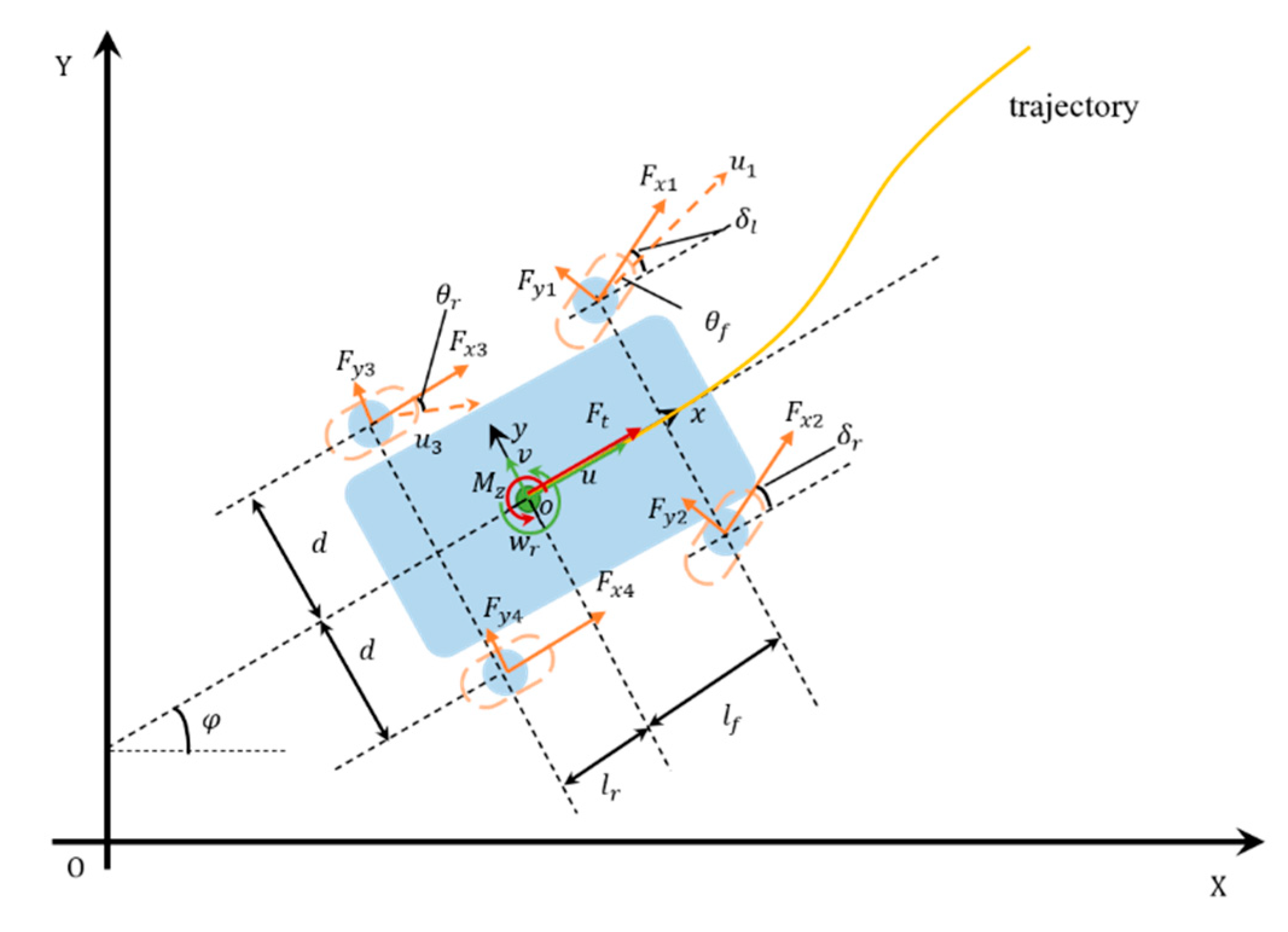
The two-track vehicle dynamic model representing the 4WID vehicle established in the Cartesian coordinate system to study the dynamic characteristics and coupling mechanism of the vehicle, as shown in Figure 1.

Assuming the small steering turning, and for simplification, the steering angles of the left and right front tires are equivalent to steering angle $\delta$ [25]. The planar motion of the vehicle can be expressed as:

$$m\ddot{x}=m\dot{y}\dot{\phi }+F_{x1}\cos \delta -F_{y1}\sin \delta +F_{x2}\cos \delta -F_{y2}\sin \delta +F_{x3}+F_{x4}-k_D{\dot{x}}^2$$

(1)

$$m\ddot{y}=-m\dot{x}\dot{\phi }+F_{x1}\sin \delta +F_{y1}\cos \delta +F_{x2}\sin \delta +F_{y2}\cos \delta +F_{y3}+F_{y4},$$

(2)

$$I_z\ddot{\phi }=l_f\left(\left(F_{x1}+F_{x2}\right)\sin \delta +\left(F_{y1}+F_{y2}\right)\cos \delta \right)+d\left(\left(F_{x1}-F_{x2}\right)\cos \delta -\left(F_{y1}-F_{y2}\right)\sin \delta +F_{x3}-F_{x4}\right)-l_r\left(F_{y3}+F_{y4}\right),$$

(3)

where the definition of each symbol is showed in

Table A1. Symbols and definitions of the dynamics model cited.

Definition	Symbol	Unit
Vehicle mass	$m$	$\mathrm{kg}$
Vehicle inertia on yaw direction	$I_z$	$\mathrm{kg}·{\mathrm{m}}^2$
Longitudinal speed/acceleration (in $xoy$)	$\dot{x}$/$\ddot{x}$	$\mathrm{m}/\mathrm{s}$
Lateral speed/acceleration (in $xoy$)	$\dot{y}$/$\ddot{y}$	$\mathrm{m}/\mathrm{s}$
Longitudinal force vector on tire (in $xoy$)	${F_x}^{\divideontimes }$	$\mathrm{N}$
Lateral force vector on tire (in $xoy$)	${F_y}^{\ast }$	$\mathrm{N}$
Distance from c.g. to the front/rear axle	$l_f$/$l_r$	$\mathrm{m}$
Length of wheelbase	$d$	$\mathrm{m}$
Longitudinal force on each tire (in tire coordinate)	$F_{xi}$	$\mathrm{N}$
Lateral force on each tire (in tire coordinate)	$F_{yi}$	$\mathrm{N}$
Front wheel steering angle on the left/right	${\delta }_{fl}$/${\delta }_{fr}$	$\mathrm{rad}$
Equivalent steering angle	$\delta$	$\mathrm{rad}$
Slip angle of the front/rear wheel	${\alpha }_f$/${\alpha }_r$	$\mathrm{rad}$
Speed angle of the front/rear wheel	${\theta }_f$/${\theta }_r$	$\mathrm{rad}$
Cornering stiffness of the front/rear wheel	$C_f$/$C_r$	$\mathrm{N}/\mathrm{rad}$
Yaw angle of vehicle body (in $\mathrm{XOY}$)	$\phi$	$\mathrm{rad}$
Total input longitudinal force on vehicle c.g.	$F_t$	$\mathrm{N}$
Total input yaw moment on vehicle c.g.	$M_z$	$\mathrm{Nm}$
Longitudinal force distribute rate on front/rear wheel	$k_f$/$k_r$	-
Aerodynamic drag coefficient	$k_d$	$\mathrm{N}/{\left(\mathrm{m}/\mathrm{s}\right)}^2$
Control error on longitudinal/lateral/yaw directions	${\mathrm{e}}_{\dot{x}}/{\mathrm{e}}_{\dot{y}}/{\mathrm{e}}_{\phi }$	$\mathrm{m}/\mathrm{s}/\mathrm{m}/\mathrm{s}/\mathrm{rad}$
Tracking error on longitudinal/lateral	${\mathrm{e}}_{\dot{X}}/{\mathrm{e}}_{\dot{Y}}$	$\mathrm{m}/\mathrm{m}$

.

When the tire force differential algorithm is adopted, the longitudinal forces are synthetically considered as the total longitudinal force $F_t$ and the additional yaw moment $M_z$ [26].

$$F_t=F_{x1}+F_{x2}+F_{x3}+F_{x4}$$

(4)

$$M_z=d\left(\Delta F\cos \delta +\Delta F\right),$$

(5)

where the longitudinal force distribution ratio of the front and rear axles $k_r$ is defined as:

$$k_r=\frac{F_{x3}+F_{x4}}{F_t},$$

(6)

The additional yaw moment $M_z$ is caused by the longitudinal force difference $\Delta F$ between the vehicle’s two sides:

$$\Delta F=F_{x1}-F_{x2}=F_{x3}-F_{x4},$$

(7)

Then, introducing the small angle hypothesis, the tire lateral force is proportional to its slip angle [27].

$${\alpha }_f= \delta -{\theta }_f=\delta -\left(\dot{y}+l_f\dot{\phi }\right)/\dot{x},$$

(8)

$${\alpha }_r= {\theta }_r=-\left(\dot{y}-l_r\dot{\phi }\right)/\dot{x},$$

(9)

The two-track model is simplified to a 3DOF model.

$$\ddot{x}=\dot{y}\dot{\phi }+\frac{F_t}{m}-\frac{k_D{\dot{x}}^2}{m}-\frac{2C_f{\delta }^2}{m}+2\frac{C_f\delta }{m}\frac{\dot{y}}{\dot{x}}+2\frac{C_f{l}_f\delta }{m}\frac{\dot{\phi }}{\dot{x}},$$

(10)

$$\ddot{y}=-\dot{x}\dot{\phi }-2\frac{C_f+C_r}{m}\frac{\dot{y}}{\dot{x}}-2\frac{C_f{l}_f-C_r{l}_r}{m}\frac{\dot{\phi }}{\dot{x}}+\frac{\left(2C_f+\left(1-k_r\right)F_t\right)\delta }{m},$$

(11)

$$\ddot{\phi }=\frac{M_z}{I_z}-2\frac{C_f{l}_f-C_r{l}_r}{I_z}\frac{\dot{y}}{\dot{x}}-2\frac{C_f{l}_f{}^2+C_r{l}_r{}^2}{I_z}\frac{\dot{\phi }}{\dot{x}}+\frac{l_f\left(1-k_r\right)F_t\delta }{I_z}+\frac{2C_f{l}_f\delta }{I_z},$$

(12)

The dynamics can be rewritten in the state-space form, with the states being $X={\left(\dot{x},\dot{y,}\dot{\phi }\right)}^T$, and the control inputs being $U={\left(F_t,\delta ,M_z\right)}^T$,i.e.,

$$\dot{X}=\left[\begin{array}{ccc}\frac{-k_D\dot{x}}{m}& \dot{\phi }& 0\\ -\dot{\phi }& -2\frac{C_f+C_r}{m\dot{x}}& -2\frac{C_f{l}_f-C_r{l}_r}{m\dot{x}}\\ 0& -2\frac{C_f{l}_f-C_r{l}_r}{I_z\dot{x}}& -2\frac{C_f{l}_f{}^2+C_r{l}_r{}^2}{I_z\dot{x}}\end{array}\right]X+\left[\begin{array}{ccc}\frac{1}{m}& 2C_f\frac{\frac{\dot{y}}{\dot{x}}+l_f\frac{\dot{\phi }}{\dot{x}}-\delta }{m}& 0\\ \frac{\left(1-k_r\right)\delta }{m}& \frac{2C_f}{m}& 0\\ \frac{l_f\left(1-k_r\right)\delta }{I_z}& \frac{2C_f{l}_f}{I_z}& \frac{1}{I_z}\end{array}\right]U,$$

(13)

In Equation (13), the input matrix is a non-diagonal matrix, which means each state of the system is affected by multiple inputs. The input matrix is not a constant coefficient matrix, but contains input elements and state elements, which indicates that there are complex interactions among three directions and causes the attendant disturbances when controlling one of the directions, such as the $-2C_f{\delta }^2/m$ is a longitudinal resistance caused by lateral control input.

Once ignoring the attendant disturbance, the control errors appear and deteriorate tracking [28]:

$$e_{\dot{X}}=e_{\dot{x}}\cos e_{\phi }+e_{\dot{y}}\sin e_{\phi },$$

(14)

$$e_{\dot{Y}}=e_{\dot{y}}\cos e_{\phi }-e_{\dot{x}}\sin e_{\phi },$$

(15)

3. Methodology

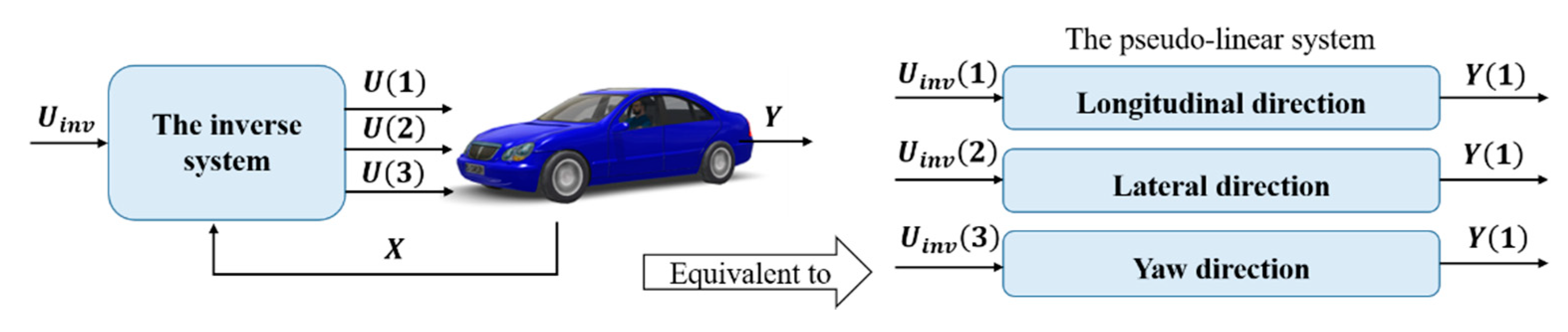
Once an inverse system whose inputs and outputs are strictly opposed to the origin system exists, the decoupling method based on the inverse system will be valid, as shown in Figure 2; that is, the inverse system and the control object are connected in series to form an equivalent multiple single-input single-output combined system without interactions.

3.1. Decoupling of Dynamics

3.1.1. Proof of Reversibility

In order to apply the decoupling algorithm, it is necessary to prove the reversibility of the vehicle dynamic. Here, the proof is derived based on the Interactor Algorithm 1 [29,30].

For a multiple-input and multiple-output (MIMO) nonlinear system, it can be written as

$$\dot{X}=f\left(X,U\right),$$

(16)

$$Y=h\left(X\right),$$

(17)

where the input vector is $U={\left[u_1,u_2\dots ,u_p\right]}^T$, the state vector is $X={\left[x_1,x_2\dots ,x_n\right]}^T$ and the output vector is $Y={\left[y_1,y_2\dots ,y_q\right]}^T={\left[h_1\left(X\right),h_2\left(X\right)\dots ,h_q\left(X\right)\right]}^T$.

Algorithm 1. Interactor Algorithm

1:    Defining the superscript $r_k$, which means taking the derivative for k-th component $y_k, r_k$ is the order when control input $U={\left[u_1,u_2\dots ,u_p\right]}^T$ firstly appears, and the derivative is noted as $y_k^{\left(r_k\right)}$

2:    For $k=1, q$

3:         Defining a criterion vector ${\Gamma }_k=\left[\begin{array}{c}{\Gamma }_{k-1}\\ y_k^{\left(r_k\right)}\end{array}\right]$, and ${\Gamma }_0$ is null when $k=1$

4:         Calculating the rank of the Jacobian matrix $R_k=rank\left(\partial {\Gamma }_k/\partial U\right)$

5:         If $R_k=k$

6:              ${\alpha }_k=r_k$

7:         End If

8:     End For

9:     If $\sum _{i=1}^k{\alpha }_k\le n$

10:       The system is reversible.

11:    End If

As for the proposed vehicle dynamics, the output vector is $Y={\left(\dot{x},\dot{y,}\dot{\phi }\right)}^T$.

Setting $y_1=\dot{x}$, which does not include any input variable, ${\Gamma }_1$ needs to be rewritten with respect to its derivative [21]: that is, ${\Gamma }_1=y_1^{\left(1\right)}=\dot{y}\dot{\phi }+\frac{F_t}{m}-\frac{k_D{\dot{x}}^2}{m}-\frac{2C_f{\delta }^2}{m}+2\frac{C_f\delta }{m}\frac{\dot{y}}{\dot{x}}+2\frac{C_f{l}_f\delta }{m}\frac{\dot{\phi }}{\dot{x}}$, the rank of the Jacobian matrix of ${\Gamma }_1$ to $U$ is

$$R_1=\mathrm{rank}\left(\partial {\Gamma }_1/\partial U\right)=\left[\begin{array}{ccc}\frac{1}{m}& 2C_f\frac{\frac{\dot{y}}{\dot{x}}+l_f\frac{\dot{\phi }}{\dot{x}}-\delta }{m}& 0\end{array}\right]=1,$$

(18)

So that, ${\alpha }_1=r_1=1$. And $y_2=\dot{y}$, which also does not include any input variable. Hence, setting ${\Gamma }_2=\left[\begin{array}{c}{\Gamma }_1\\ y_2^{\left(1\right)}\end{array}\right]=\left[\begin{array}{c}\ddot{x}\\ \ddot{y}\end{array}\right]$,

$$R_2=\mathrm{rank}\left(\partial {\Gamma }_2/\partial U\right)=\left[\begin{array}{ccc}\frac{1}{m}& 0& 0\\ \frac{\left(1-k_r\right)\delta }{m}& \frac{2C_f}{m}& 0\end{array}\right]=2,$$

(19)

we can get that ${\alpha }_2=r_2=1$. At last, setting ${\Gamma }_3=\left[\begin{array}{c}{\Gamma }_2\\ y_3^{\left(1\right)}\end{array}\right]=\left[\begin{array}{c}\ddot{x}\\ \ddot{y}\\ \ddot{\phi }\end{array}\right]$,

$${\mathrm{R}}_3=rank\left(\partial {\Gamma }_3/\partial \Gamma \right)=\left[\begin{array}{ccc}\frac{1}{m}& 2C_f\frac{\frac{\dot{y}}{\dot{x}}+l_f\frac{\dot{\phi }}{\dot{x}}-\delta }{m}& 0\\ \frac{\left(1-k_r\right)\delta }{m}& \frac{2C_f}{m}& 0\\ \frac{l_f\left(1-k_r\right)\delta }{I_z}& \frac{2C_f{l}_f}{I_z}& \frac{1}{I_z}\end{array}\right]=3,$$

(20)

and this yields ${\alpha }_3=r_3=1$, then

$${\displaystyle \sum }_{i=1}^3{\alpha }_3=3,$$

(21)

According to the reversibility judgment [31], there is an inverse system for the 4WID vehicle without hidden dynamics [32], and the input and output of the inverse system are $U_{inv}={\left(y_1^{\left(1\right)},y_2^{\left(1\right)},y_3^{\left(1\right)}\right)}^T={\left(\ddot{x},\ddot{y},\ddot{\phi }\right)}^T$ and $Y_{inv}={\left(F_t,\delta ,M_z\right)}^T$.

As the 3DOF vehicle dynamic system is reversible and based on the Equation (13), the inverse system can be written as Equation (22):

$$\begin{gathered} Y_{inv}=-{\left[\begin{array}{ccc}\frac{1}{m}& 2C_f\frac{\frac{\dot{y}}{\dot{x}}+l_f\frac{\dot{\phi }}{\dot{x}}-\delta }{m}& 0\\ \frac{\left(1-k_r\right)\delta }{m}& \frac{2C_f}{m}& 0\\ \frac{l_f\left(1-k_r\right)\delta }{I_z}& \frac{2C_f{l}_f}{I_z}& \frac{1}{I_z}\end{array}\right]}^{-1}\left[\begin{array}{ccc}\frac{-k_D\dot{x}}{m}& \dot{\phi }& 0\\ -\dot{\phi }& -2\frac{C_f+C_r}{m\dot{x}}& -2\frac{C_f{l}_f-C_r{l}_r}{m\dot{x}}\\ 0& -2\frac{C_f{l}_f-C_r{l}_r}{I_z\dot{x}}& -2\frac{C_f{l}_f{}^2+C_r{l}_r{}^2}{I_z\dot{x}}\end{array}\right]X \\ +{\left[\begin{array}{ccc}\frac{1}{m}& 2C_f\frac{\frac{\dot{y}}{\dot{x}}+l_f\frac{\dot{\phi }}{\dot{x}}-\delta }{m}& 0\\ \frac{\left(1-k_r\right)\delta }{m}& \frac{2C_f}{m}& 0\\ \frac{l_f\left(1-k_r\right)\delta }{I_z}& \frac{2C_f{l}_f}{I_z}& \frac{1}{I_z}\end{array}\right]}^{-1}{U}_{inv} \end{gathered}$$

(22)

3.1.2. Definition of the Inverse System

As shown in Equation (22), the output can be calculated using the Taylor series expansion. However, to avoid the approximation error caused by the omission of high-order terms in the Taylor formula, a machine learning method is applied to identify the relationship between the input and output of the system in this paper. Because the identification of the inverse system is a MIMO regression, the back propagation neural network (BPNN) model is adopted. Note that $\ddot{x}$ and $\ddot{y}$ are replaced by the measurable $a_x$ and $a_y$:

$$\ddot{x}=a_x+\dot{y}\dot{\phi },$$

(23)

$$\ddot{y}=a_y-\dot{x}\dot{\phi },$$

(24)

Hence, the input and output of the BPNN model are $U_{nn}={\left(a_x,a_y,\ddot{\phi },\dot{x},\dot{y,}\dot{\phi }\right)}^T$ and $Y_{nn}={\left(F_t,\delta ,M_z\right)}^T$.

3.1.3. Neural Networks Training

The D-class sedan model of CarSim is utilized to obtain the vehicle responses $\left\{a_x,a_y,\ddot{\phi },\dot{x},\dot{y,}\dot{\phi }\right\}$ under stochastic inputs $\left\{F_t,\delta ,M_z\right\}$. To simulate the 4WID vehicle, the total longitudinal force and yaw moment are converted to driven torques of each wheel based on Equations (2) and (4).

$$T_{fl,fr}=\frac{\left(1-k_r\right)F_t\mp M_z/d\left(1+\cos \delta \right)}{r}+I_r\frac{d{w}_{fl,fr}}{dt},$$

(25)

$$T_{rl,rr}=\frac{k_r{F}_t\mp M_z/d\left(1+\cos \delta \right)}{r}+I_r\frac{d{w}_{fl,fr}}{dt},$$

(26)

where $T_{fl}$, $T_{fl}$, $T_{fl}$, $T_{fl}$ are the driven torques of the front-left, front-right, rear-left and rear-right tire, respectively. $r$ is the radius of each wheel. $I_r$ is the wheel inertia moment. $w_{fl,fr}$ and $w_{fl,fr}$ are the rotation velocities of each wheel.

The longitudinal and lateral acceleration were constrained considering the ride comfort and anti-sideslip [33].

$$-{\eta }_{d}g\le a_x\le \eta g,$$

(27)

$$-{\mu }_{s}g\le a_y\le {\mu }_{s}g,$$

(28)

where ${\eta }_d$, $\eta$ and ${\mu }_s$ respectively represent the maximum coefficient of longitudinal deceleration, longitudinal acceleration and lateral acceleration. According to the vehicle dynamics and the kinematic model:

$$a_x=\frac{F_t}{m},$$

(29)

$$R=\frac{L}{\sin \left|\delta \right|}\approx \frac{L}{\left|\delta \right|},$$

(30)

where $R$ is the turning radius of the vehicle, and $L$ is the distance between the front and rear axles. Then, substituting Equations (29) and (30) into Equations (27) and (28) yields:

$$\left|\delta \right|\le \frac{{\mu }_{s}gL}{u^2},$$

(31)

$$-\mu mg\le F_t\le \mu mg,$$

(32)

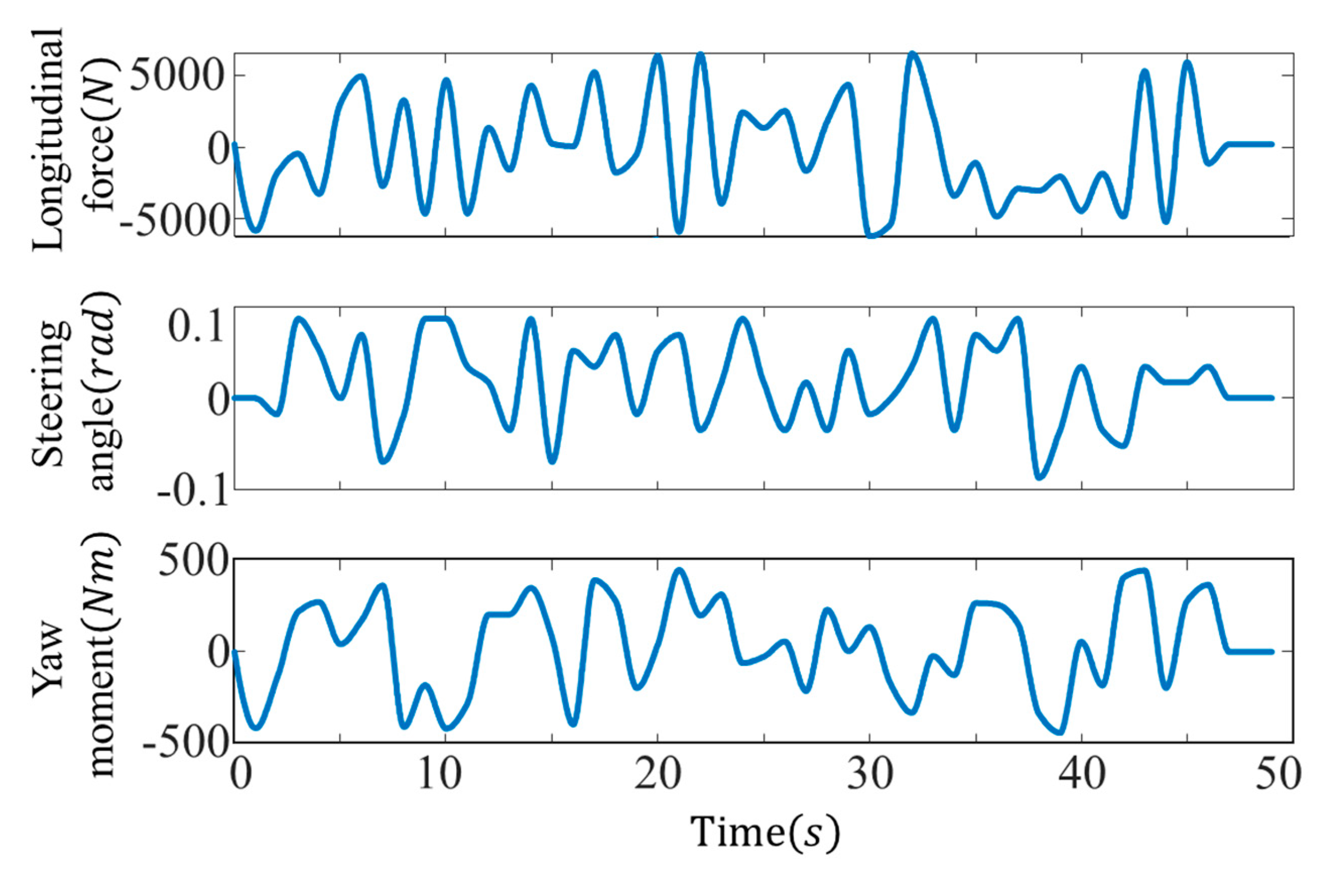
The interval between two sampling points of longitudinal force, steering angle and additional yaw moment is 2 s. The values of sampling points are stochastically generated, obeying the uniform distribution in the range of $\left(-5000,5000\right)N$, $\left(-0.1,0.1\right)rad$ and $\left(-500,500\right)Nm$, respectively. The sampling data are interpolated by the Hermite method for smoothness, as shown in Figure 3.

By setting different initial speeds, multiple groups of input signals act on the vehicle model, then the inputs and the responses of the vehicle are recorded as the training dataset. To ensure the validity of the collected data set, the following two constraints need to be guaranteed.

• The equivalent steering angle is constrained according to the real-time speed.
• The vehicle speed is always positive.

3.1.4. Design of the Trajectory Tracking Controller

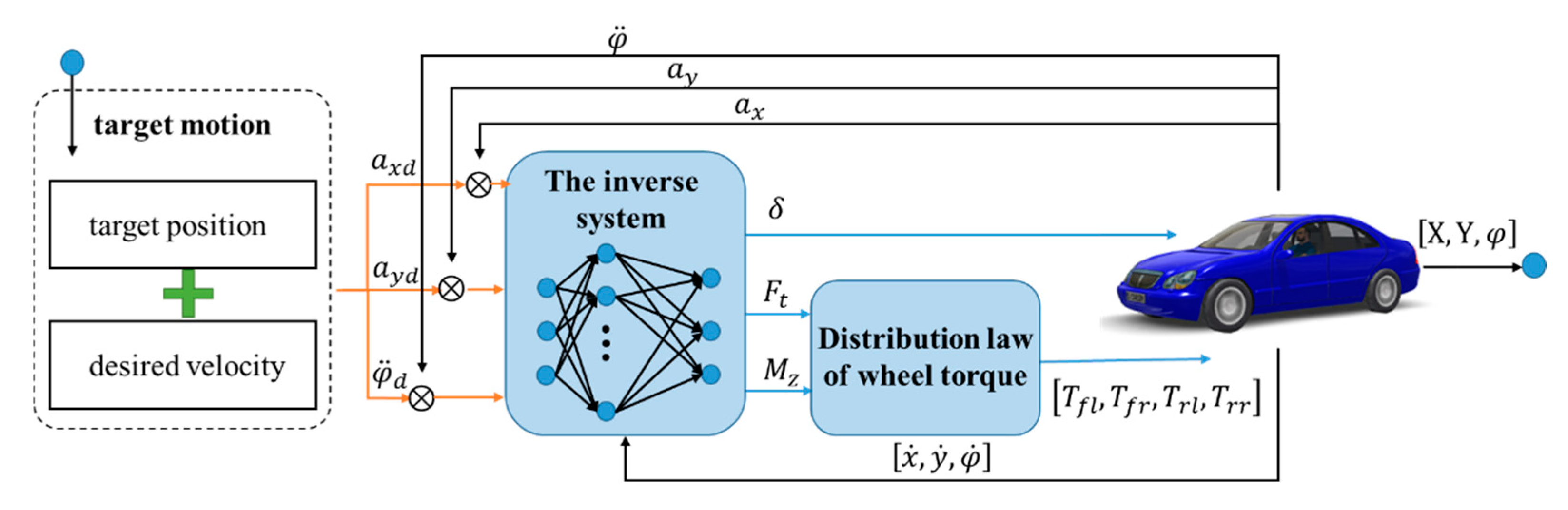
Based on the inverse system, the control framework is built in Figure 4. The target motion trajectory transformed into the vehicle dynamic state references—that is, the longitudinal acceleration, the lateral acceleration, and the yaw acceleration. By following the target vehicle dynamic state, the inverse system exports the vehicle inputs and drives the vehicle tracking desired trajectory.

3.2. The Desired Vehicle States

Based on the kinematic model, the desired vehicle states, i.e., the references of the inverse system $U_{ref}=\left(a_x,a_y,\ddot{\phi }\right)$, are calculated from the target motion trajectory.

Supposing that the references from the planning module are the sequences of resultant speed $V\left(t\right)$ and trajectory $Y\left(X\right)$, $t$ is the time, $X$ and $Y$ are the vehicle longitudinal and lateral position in the inertial coordinate system.

The spatial–temporal relationship is unified by using the travel distance of vehicles [34].

$${\displaystyle \int }Vdt={\displaystyle \sum }_i^n\sqrt{\Delta X{\left(i\right)}^2+\Delta Y{\left(i\right)}^2},$$

(33)

where $\Delta X\left(i\right)$ and $\Delta Y\left(i\right)$ are the longitudinal and lateral spacing between the $i+1$ th point and the $i$ th point in the inertial coordinate system.

The desired yaw can be calculated as [35]:

$$\phi \left(i\right)={\tan }^{-1}\frac{\Delta Y\left(i\right)}{\Delta X\left(i\right)},$$

(34)

The vehicle velocity along the $X$ and $Y$ directions in the inertial coordinate system are

$$V_X\left(i\right)=\frac{\Delta X\left(i\right)}{\Delta t\left(i\right)}, V_Y\left(i\right)=\frac{\Delta Y\left(i\right)}{\Delta t\left(i\right)},$$

(35)

Then, the vehicle longitudinal and lateral velocities are [28]

$$\dot{x}\left(i\right)=V_X\left(i\right)\cos \phi \left(i\right)+\Delta Y\left(i\right)\sin \phi \left(i\right),$$

(36)

$$\dot{y}\left(i\right)=-V_X\left(i\right)\sin \phi \left(i\right)+\Delta Y\left(i\right)\cos \phi \left(i\right),$$

(37)

The longitudinal, lateral and yaw accelerations are yields:

$$a_x\left(i\right)=\frac{\dot{x}\left(i\right)}{\Delta t\left(i\right)}-\dot{y}\left(k\right)\frac{\Delta \phi \left(i\right)}{\Delta t\left(i\right)},$$

(38)

$$a_y\left(i\right)=\frac{\dot{y}\left(i\right)}{\Delta t\left(i\right)}+\dot{x}\left(k\right)\frac{\Delta \phi \left(i\right)}{\Delta t\left(i\right)},$$

(39)

$$\ddot{\phi }\left(i\right)=\frac{\Delta \frac{\Delta \phi \left(i\right)}{\Delta t\left(i\right)}}{\Delta t\left(i\right)},$$

(40)

So far, the input of the inverse system, the target motion states of the vehicle $U_{ref}={\left[a_x,a_y,\ddot{\phi }\right]}^T$, has been obtained.

4. Simulation Results and Analysis

The simulations are conducted to verify the correctness of the inverse system identification and assess the tracking performance of the proposed method. A D-Class CarSim vehicle model is adopted, and the parameters are shown in

Table A2. Symbols and definitions of the dynamics model cited.

Parameters	Definition	Value
$m$	Vehicle mass	1370 $\mathrm{kg}$
$l_f$	Horizontal distance from c.g. to front tires	1.11 $\mathrm{m}$
$l_r$	Horizontal distance from c.g. to rear tires	1.67 $\mathrm{m}$
$k_D$	The resistance coefficient of air	0.35
$C_f$	cornering stiffness of front tires	67553 $\mathrm{Nm}/\mathrm{rad}$
$C_r$	cornering stiffness of rear tires	49506 $\mathrm{Nm}/\mathrm{rad}$
$I_z$	Yaw inertia	2315.3 $\mathrm{kg}/{\mathrm{m}}^2$

. The proposed trajectory tracking controller is developed in Simulink. The Simulink–CarSim interface is shown in Figure 4.

4.1. Verification of the Inverse System Models

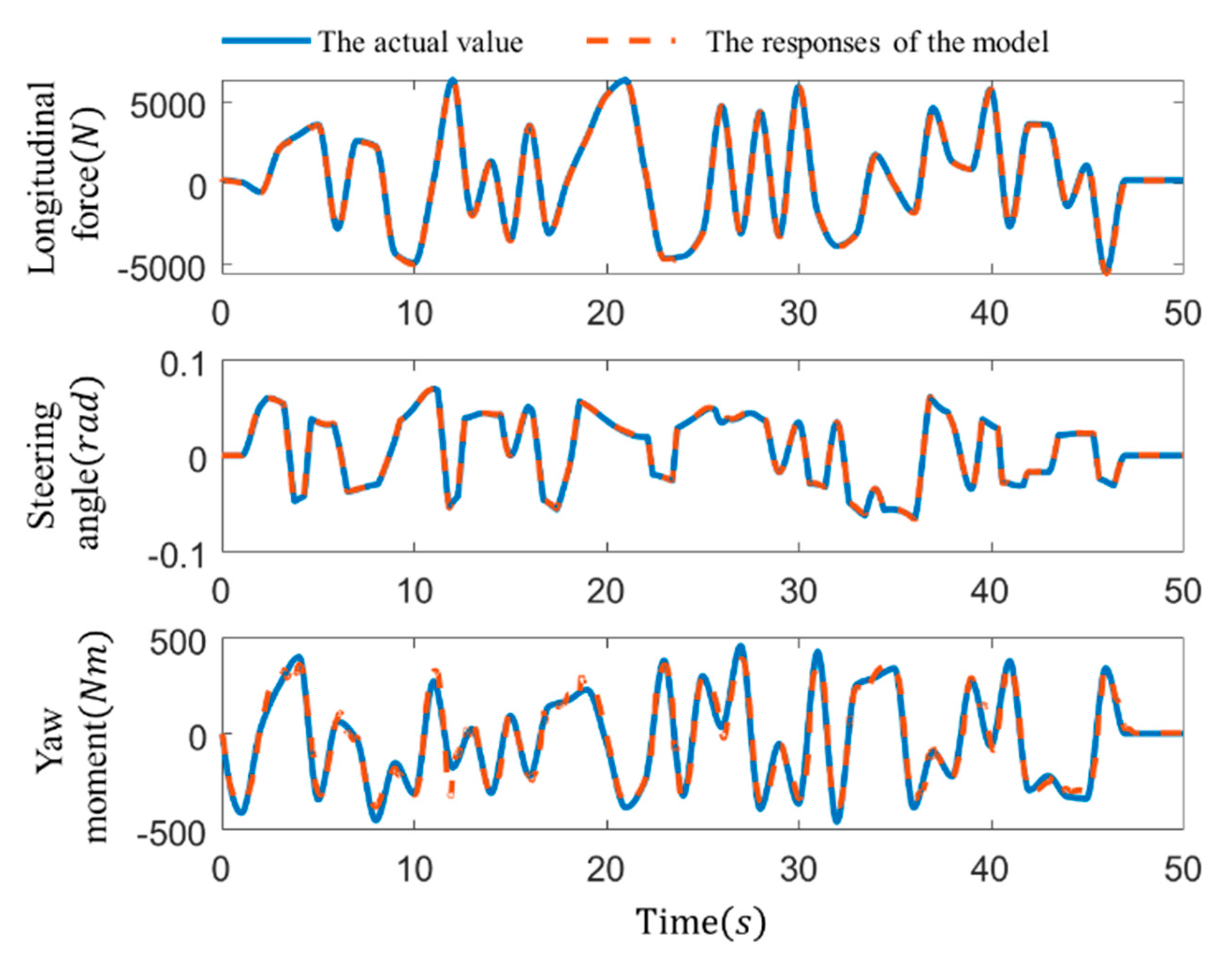
The inverse system is identified by a BPNN model whose structure is 6-50-50-3, i.e., the model has six inputs, three outputs and two hidden layers with 50 nodes. The mean square error between the training data and the prediction of the BPNN is 0.000213 and the regression factor of the model is 0.99941, which indicates that the model has identified the input–output mapping relationship between the of the inverse system. A novel test dataset was collected and applied to evaluate the fitting performance of the inverse system as Figure 5.

As shown in Figure 5, three responses of the BPNN model highly coincide with the actual value, illustrating that the identification of the inverse system is correct and the 4WID vehicle system is reversible.

4.2. Verification of Tracking Performance

Three coupling scenarios were designed to assess the tracking performance, and pure-pursuit and MPC are implemented as the benchmark to compare the improvement of the proposed method. Note that, to filter out the varying-velocity disturbance, the lateral preview reference of MPC and pure-pursuit is based on time, and a speed preview controller supplemented in parallel.

4.2.1. Scenario 1: Lane Change with Deceleration on Dry Road Surface

In this scenario, the vehicle drives at the initial speed of 90 km/h on a straight and dry road with the road adhesion coefficient being 0.8, then the decelerating lane change is completed within 58 m, which is a classic collision avoidance scenario.

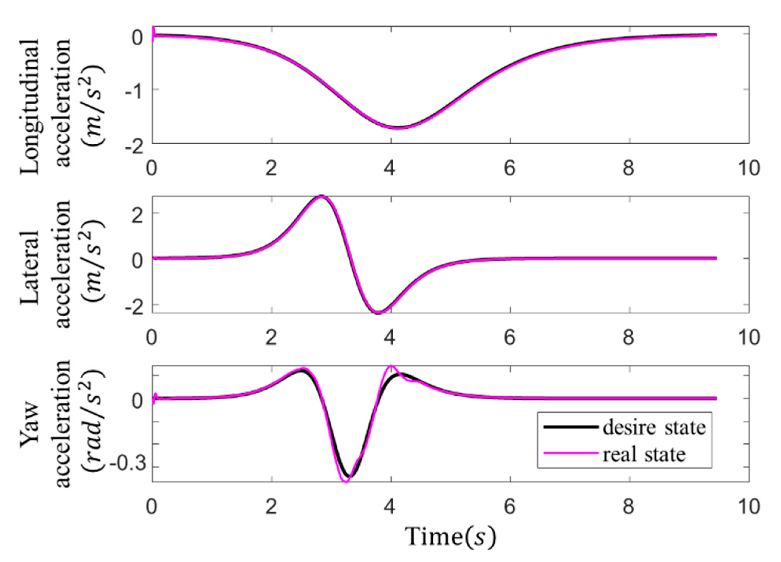
Based on the proposed method, the desired vehicle motion states $U_{ref}={\left[a_x\left(t\right),a_y\left(t\right),\ddot{\phi }\left(t\right)\right]}^T$ were calculated and the vehicle dynamic states tracking results are shown as Figure 6.

Figure 6 shows that the longitudinal acceleration, lateral acceleration of the vehicle coincide with the desired value and the change in each direction does not affect the other directions, indicating that the proposed method has decoupled dynamics and the vehicle dynamic states can be accurately tracked in close loop.

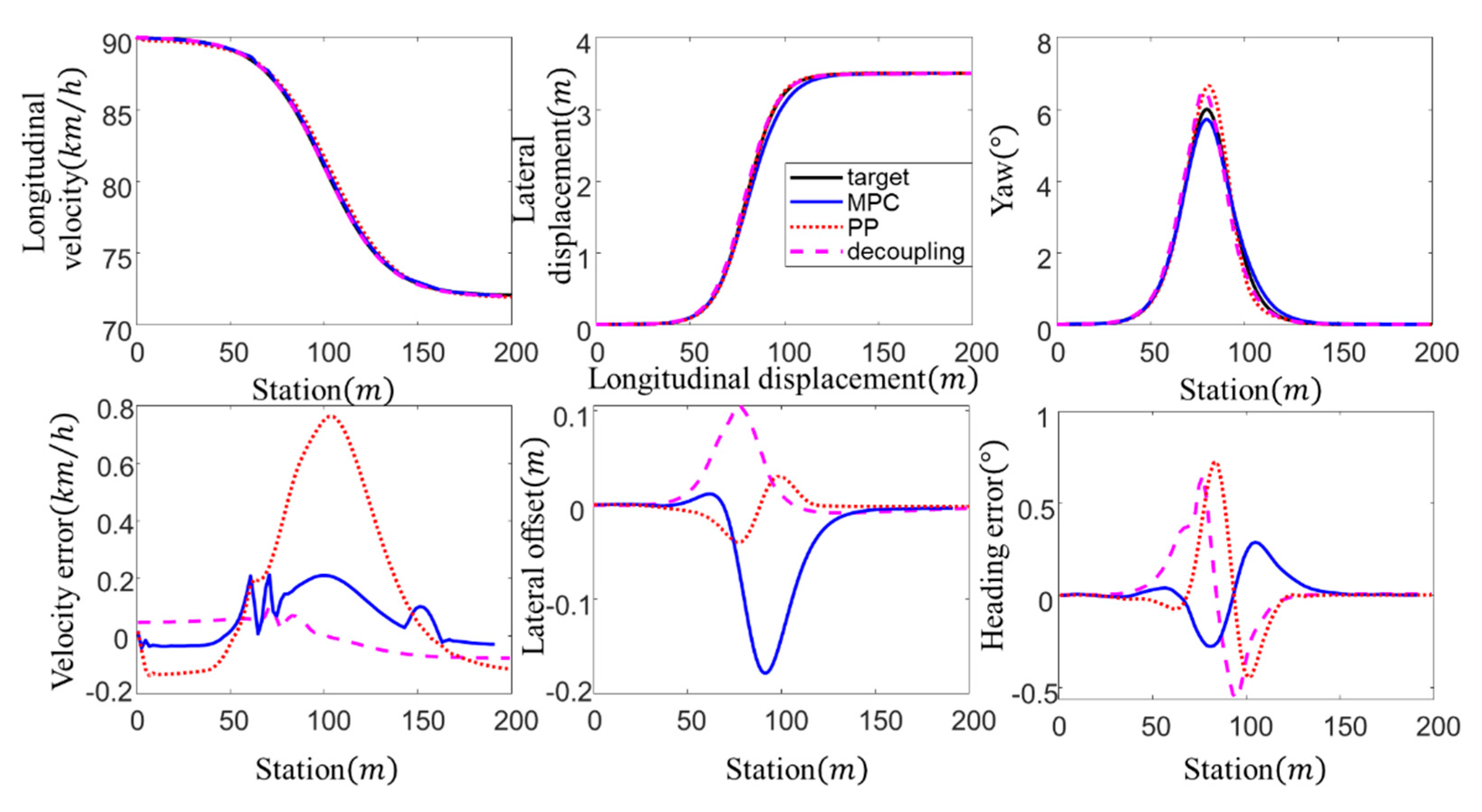
As shown in Figure 7, the real vehicle velocity and lateral position accurately follow the references. The velocity tracking error of the proposed method is smallest compared with pure-pursuit control and MPC. With the same longitudinal controller, MPC and pure-pursuit control still contribute to different speed errors, which means the longitudinal control is affected by control in other directions. Even though the lateral control value was correctly calculated by MPC, the longitudinal tracking error results in a delay in the lateral tracking owning to the lateral reference related to the time and does not consider the longitudinal error within a planning cycle, which is another deterioration of tracking accuracy caused by dynamic coupling.

To quantitatively evaluate the tracking performance of the three methods, the results were statistically analyzed.

The statistical values of lateral error are shown in

Table 1. The tracking performance statistics.

	Unit	Decoupling Control	MPC	PP
$\max \left(e_Y\right)$	$\mathrm{m}$	0.1054	0.0113	0.0296
$\min \left(e_Y\right)$	$\mathrm{m}$	−0.0090	−0.1795	−0.0399
$MS{E}_V$	${\mathrm{m}}^2/{\mathrm{s}}^2$	0.0033	0.0110	0.1164
$MS{E}_Y$	${\mathrm{m}}^2$	0.0011	0.0036	0.0002
$MS{E}_{yaw}$	${°}^2$	0.0382	0.0127	0.0386

. Compared with pure-pursuit and MPC, the mean square error of velocity ($MS{E}_V$) of the proposed method is the smallest, and its mean square error of lateral tracking ($MS{E}_Y$) and yaw tracking ($MS{E}_{yaw}$) rank in the middle.

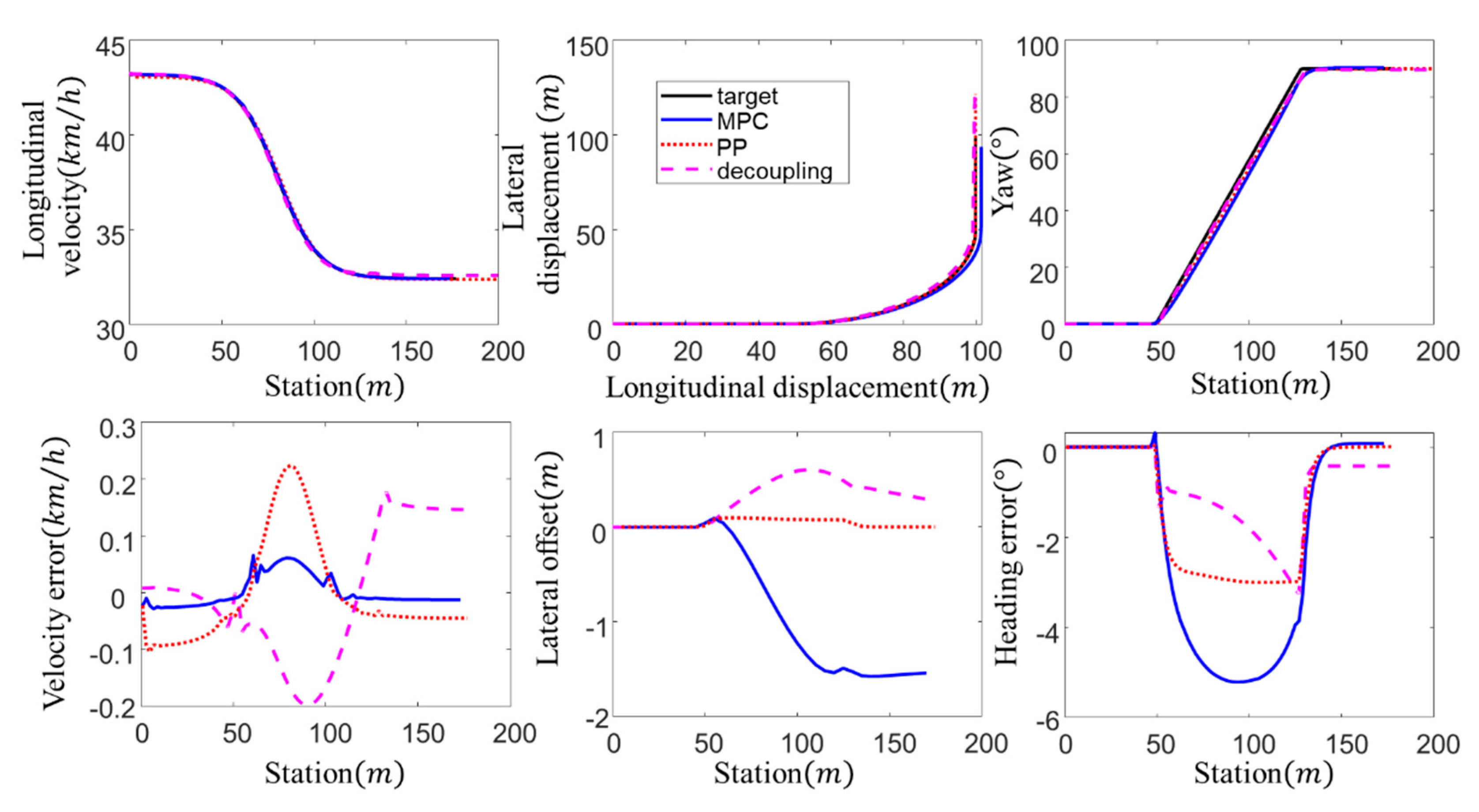
4.2.2. Scenario 2: Turn Left with Deceleration at Crossing

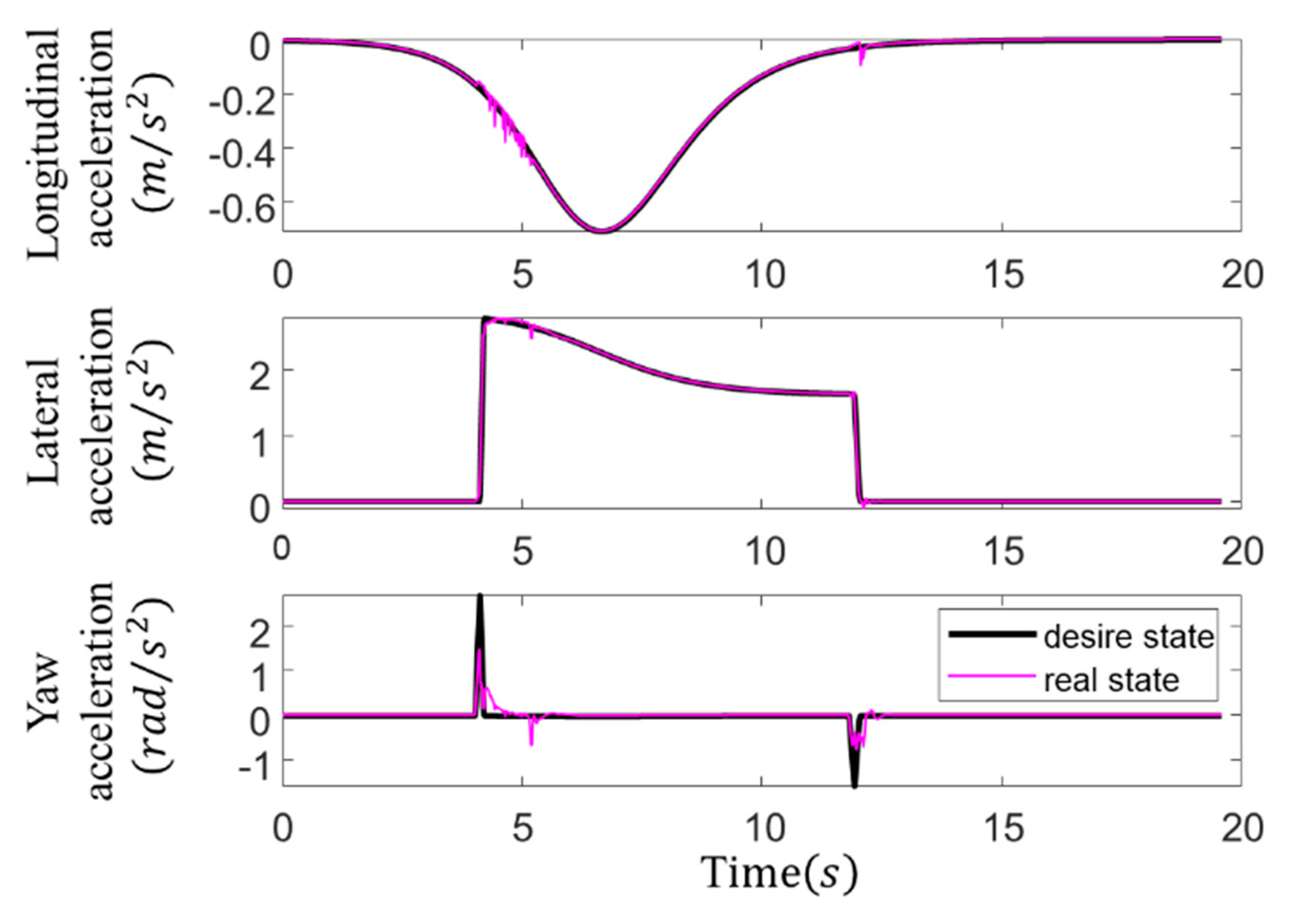
In urban traffic, the intersection is a common scene. The vehicle is required to slow down through a right-angle bend with a radius of 50 m. On a dry road with a road adhesion coefficient of 0.8, the vehicle speed decelerates to 9 m/s from 12 m/s within 5 s.

Figure 8 shows that there are two big pulses in the target $\dot{w_r}$ which are caused by the noncontinuous curvature. As the pulses with large rates of change exceeded the range of the training set, the target $\dot{w_r}$ was difficult to track and resulted in a chain reaction in the longitudinal and lateral directions. However, the longitudinal and lateral fluctuations accompanied by yaw pulses do not mean decoupling failure, because besides the fluctuating part, the other targets in the three motion directions are accurately tracked without interferences. This gives us two inspirations; first, the target vehicle motion states should be smooth and remain within the range of the training set; the other is that the curvature of the target position curve designed by the planning level should be as continuous as possible.

Figure 9 shows that the proposed method realizes the velocity, position and yaw tracking simultaneously. The fluctuations in $a_x$ and $a_y$ are amplified and accumulated, resulting in a stable velocity and lateral error of 0.193 $\mathrm{km}/\mathrm{h}$ and 0.36 $\mathrm{m}$ after a 150 $\mathrm{m}$ trip. As the lateral error is seriously related to driving safety, the tracking performance of pure-pursuit is the best in this scenario. The MPC failed to reduce the error in the $\mathrm{X}$ direction of the Cartesian coordinate system without coordinate transformation, which leads to a larger lateral error in the vehicle coordinate system.

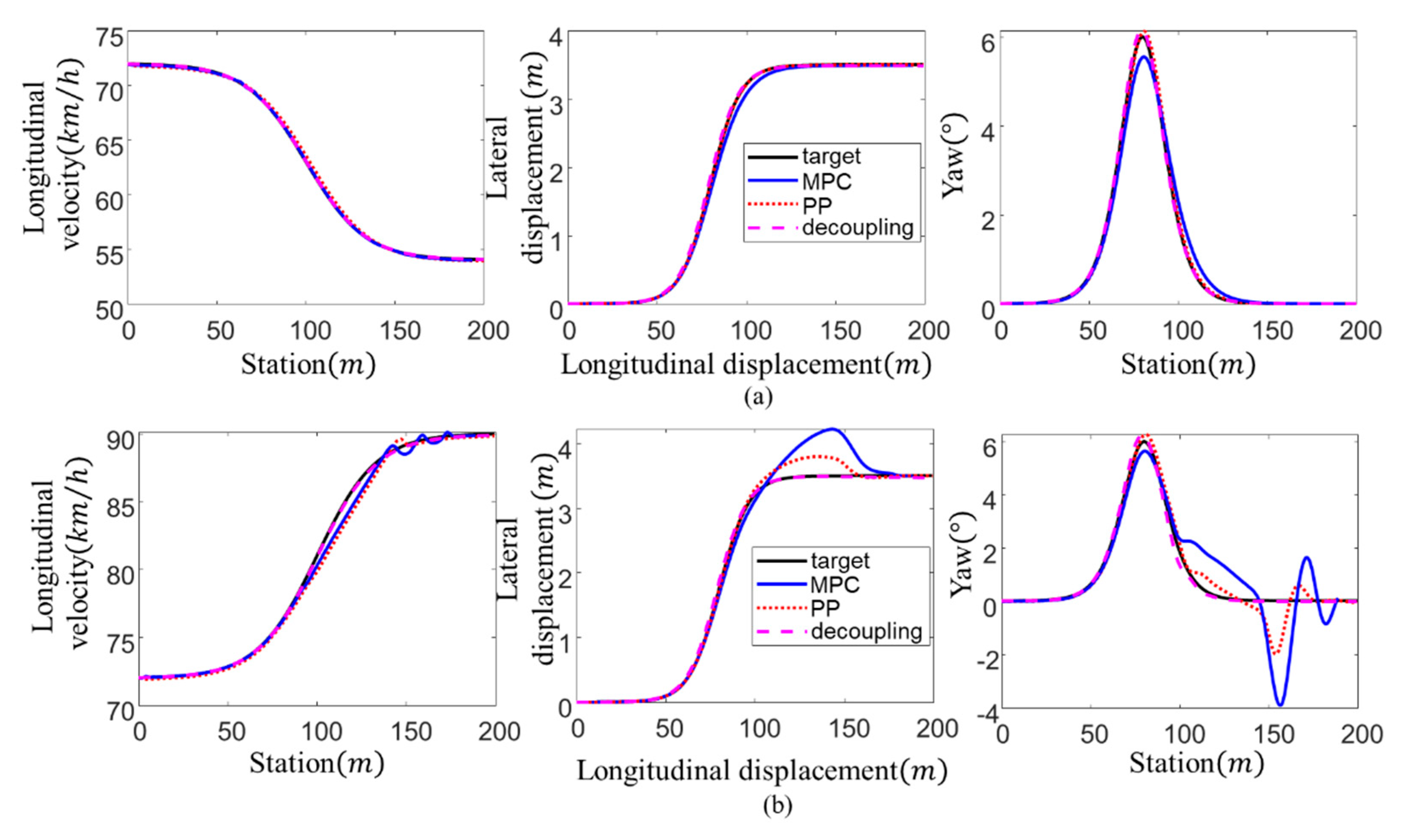
4.2.3. Scenario 3: Lane Change with Deceleration/Acceleration on a Wet Road Surface

In scenario 3, the vehicle decelerates or accelerates at the initial speed of 20 m/s when changing lane on a wet road whose road adhesion coefficient is 0.35.

Figure 10a shows that the three methods all still achieve trajectory tracking on a low-adhesion road. Compared with Figure 7, even though the road conditions are worse, the lateral and yaw tracking errors of the proposed method decrease with speed reduction. However, the lateral and yaw tracking performance of the MPC get worse. In Figure 10b, the pure-pursuit and MPC fail to track the target in longitudinal, lateral and yaw motion. However, the proposed method still follows the constrained vehicle states at the lower-adhesion road condition, guaranteeing the driving stability.

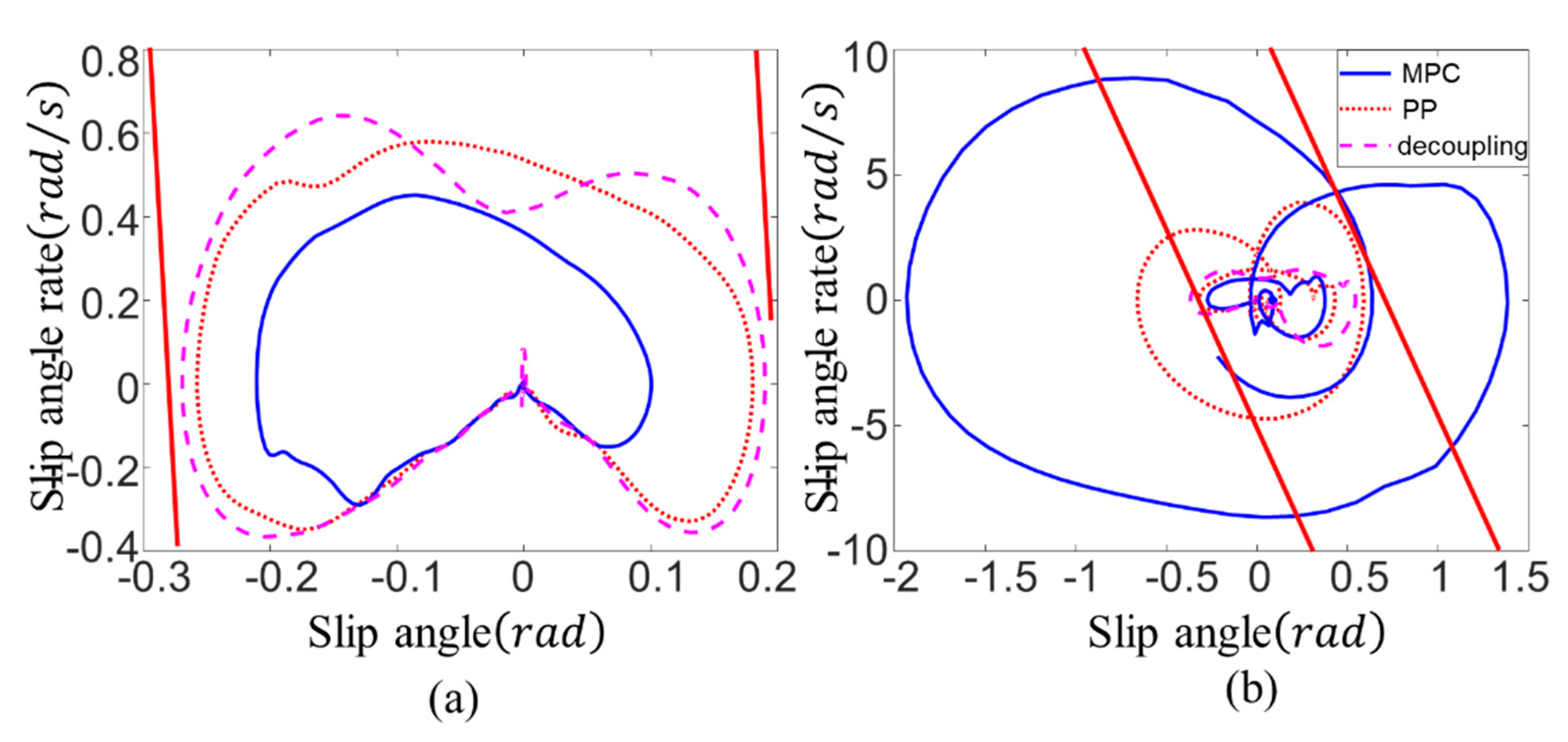
As we can see from Figure 11a, the proposed method always keeps the vehicle in the safe area of the sideslip phase-plane like the pure-pursuit and MPC; however, in Figure 11b, since the tracking performance becomes worse, the phase curve of the pure-pursuit and MPC are over the stability boundaries, which means that the proposed method significantly improves the handling stability and has fewer tracking errors compared with the pure-pursuit and MPC algorithms.

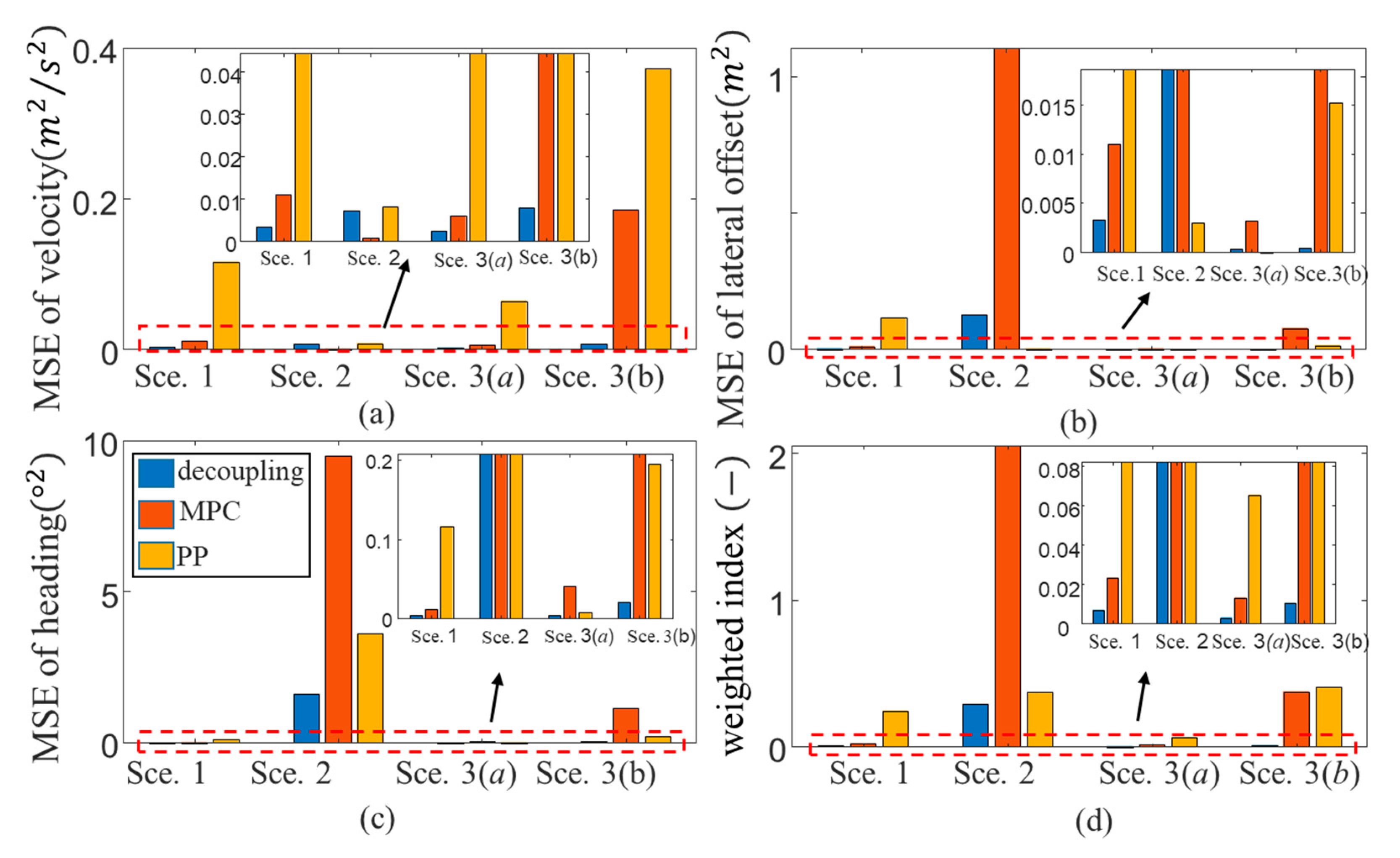
Figure 12 shows the error statistics results of the longitudinal, lateral and yaw directions of the three tracking controllers under four working conditions, as well as the trajectory tracking error index $P$ of the planar motion weighted by the three directions.

$$P=w_{1}MS{E}_V+w_{2}MS{E}_Y+w_{3}MS{E}_{yaw},$$

(41)

Considering that three directions are equally important in planar motion tracking, the three weights should be the same. However, due to the unit, the mean square error of yaw tracking is very large, so it is reduced by a certain proportion and the weighted vector is $w={\left(1,1,pi/180\right)}^T$.

As shown in Figure 12a, except for scenario 2, the $MS{E}_V$ of the proposed method is the smallest. The accurate velocity tracking illustrates that the dynamic decoupling of the proposed tracking method can effectively reduce the longitudinal interference from other motion directions. Moreover, compared with the other two methods, the proposed method still performs well in the lateral and yaw tracking. In summary, as shown in Figure 12d, the trajectory tracking error index of the proposed method proposed is always the lowest, indicating that the proposed tracking method is more suitable for performing trajectory tracking tasks under the coupled conditions than the other two methods.

5. Conclusions

To achieve the high trajectory tracking precision in the dynamic coupling scenarios, a simultaneous trajectory tracking and stability control method for 4WID automated electric vehicles is present in this paper based on the inverse system theorem. To reveal the coupling mechanism and to prove the reversibility of 4WID vehicles, the 3DOF vehicle dynamic model is constructed. The inverse system learned by a BPNN model shows effectiveness to realize dynamic decoupling. The pseudo linear system composed of the inverse system and the controlled object follows the desired vehicle dynamic states to indirectly achieve trajectory tracking. Three typical and common coupled driving conditions are designed to verify the trajectory tracking accuracy under the simultaneous control of vehicles’ longitudinal, lateral and yaw motion. Compared with the pure-pursuit algorithm and the MPC algorithm, the proposed method reduces interactions among vehicle motion directions and reveals better tracking performance. Moreover, since the target states of the vehicle have been constrained within a reasonable range, the decoupling method not only maintains the accurate trajectory tracking but also guarantees the stable vehicle driving under low-adhesion road conditions. Even though the proposed method theoretically shows better control performance, further verifications could be implemented on real vehicles to realize the engineering applications.

References

- Xu, S.; Peng, H. Design, Analysis, and Experiments of Preview Path Tracking Control for Autonomous Vehicles. IEEE Trans. Intell. Transp. Syst. 2020, 21, 48–58. [Google Scholar] [CrossRef]
- Wang, Y.; Shao, Q.; Zhou, J. Longitudinal and lateral control of autonomous vehicles in multi-vehicle driving environments. IET Intell. Transp. Syst. 2020, 14, 924–935. [Google Scholar] [CrossRef]
- Chen, T.; Chen, L.; Xu, X.; Cai, Y. Simultaneous path following and lateral stability control of 4WD-4WS autonomous electric vehicles with actuator saturation. Adv. Eng. Softw. 2019, 128, 46–54. [Google Scholar] [CrossRef]
- Samuel, M.; Hussein, M.; Mohamad, M. A Review of some Pure-Pursuit based Path Tracking Techniques for Control of Autonomous Vehicle. Int. J. Comput. Appl. 2016, 135, 35–38. [Google Scholar] [CrossRef]
- Wang, R.; Ye, Q.; Cai, Y. Analyzing the influence of automatic steering system on the trajectory tracking accuracy of intelligent vehicle. Adv. Eng. Softw. 2018, 121, 188–196. [Google Scholar] [CrossRef]
- Thrun, S.; Montemerlo, M.; Dahlkamp, H. Stanley: The Robot That Won the DARPA Grand Challenge. J. Field Robot. 2006, 23, 661–692. [Google Scholar] [CrossRef]
- Falcone, P.; Borrelli, F.; Asgari, J. Predictive active steering control for autonomous vehicle systems. IEEE Trans. Control Syst. Technol. 2007, 15, 566–580. [Google Scholar] [CrossRef]
- Yu, Z.; Zhang, R.; Xiong, L. Robust hierarchical controller with conditional integrator based on small gain theorem for reference trajectory tracking of autonomous vehicles. Veh. Syst. Dyn. 2019, 57, 1143–1162. [Google Scholar] [CrossRef]
- Talvala, K.L.; Kritayakirana, K.; Gerdes, J.C. Pushing the limits: From lanekeeping to autonomous racing. Annu. Rev. Control. 2011, 35, 137–148. [Google Scholar] [CrossRef]
- Ni, J.; Hu, J. Dynamics control of autonomous vehicle at driving limits and experiment on an autonomous formula racing car. Mech. Syst. Signal Process. 2017, 90, 154–174. [Google Scholar] [CrossRef]
- Brown, M.; Funke, J.; Erlien, S.M. Safe driving envelopes for path tracking in autonomous vehicles. Control Eng. Pract. 2017, 61, 307–316. [Google Scholar] [CrossRef]
- Ji, J.; Khajepour, A.; Melek, W.W. Path planning and tracking for vehicle collision avoidance based on model predictive control with multiconstraints. IEEE Trans. Veh. Technol. 2017, 66, 952–964. [Google Scholar] [CrossRef]
- Turri, V.; Carvalho, A.; Tseng, H.E. Linear model predictive control for lane keeping and obstacle avoidance on low curvature roads. In Proceedings of the 16th international IEEE conference on intelligent transportation systems (ITSC 2013), The Hague, The Netherlands, 6–9 October 2013; pp. 378–383. [Google Scholar]
- Attia, R.; Orjuela, R.; Basset, M. Combined longitudinal and lateral control for automated vehicle guidance. Veh. Syst. Dyn. 2014, 52, 261–279. [Google Scholar] [CrossRef] [Green Version]
- Kanayama, Y.; Kimura, Y.; Miyazaki, F. A stable tracking control method for an autonomous mobile robot. In Proceedings of the IEEE International Conference on Robotics and Automation, Cincinnati, OH, USA, 13–18 May 1990; pp. 384–389. [Google Scholar]
- Menhour, L.; Dandreanovel, B.; Fliess, M. Coupled nonlinear vehicle control: Flatness-based setting with algebraic estimation techniques. Control Eng. Pract. 2014, 22, 135–146. [Google Scholar] [CrossRef] [Green Version]
- Gao, Y.; Gray, A.; Tseng, H.E. A tube-based robust nonlinear predictive control approach to semiautonomous ground vehicles. Veh. Syst. Dyn. 2014, 52, 802–823. [Google Scholar] [CrossRef]
- Brown, M.; Gerdes, J.C. Coordinating tire forces to avoid obstacles using nonlinear model predictive control. IEEE Trans. Intell. Veh. 2020, 5, 21–31. [Google Scholar] [CrossRef]
- Marino, R.; Scalzi, S. Asymptotic sideslip angle and yaw rate decoupling control in four-wheel steering vehicles. Veh. Syst. Dyn. 2010, 48, 999–1019. [Google Scholar] [CrossRef]
- Zhang, H.; Zhao, W. Decoupling control of steering and driving system for in-wheel-motor-drive electric vehicle. Mech. Syst. Signal Process. 2018, 101, 389–404. [Google Scholar] [CrossRef]
- Wang, C.; Zhao, W.; Luan, Z. Decoupling control of vehicle chassis system based on neural network inverse system. Mech. Syst. Signal Process. 2018, 106, 176–197. [Google Scholar] [CrossRef]
- Hu, C.; Wang, R.; Yan, F. Should the desired heading in path following of autonomous vehicles be the tangent direction of the desired path. IEEE Trans. Intell. Transp. Syst. 2015, 16, 3084–3094. [Google Scholar] [CrossRef]
- Li, B.; Du, H.; Li, W. Trajectory control for autonomous electric vehicles with in-wheel motors based on a dynamics model approach. IET Intell. Transp. Syst. 2016, 10, 318–330. [Google Scholar] [CrossRef]
- Ge, S.S.; Cui, Y.J. Dynamic motion planning for mobile robots using potential field method. Auton. Robot. 2002, 13, 207–222. [Google Scholar] [CrossRef]
- Lin, F.; Zhang, Y.; Zhao, Y. Trajectory Tracking of Autonomous Vehicle with the Fusion of DYC and Longitudinal–Lateral Control. Chin. J. Mech. Eng. 2019, 32, 16. [Google Scholar] [CrossRef]
- Wu, J.; Cheng, S.; Liu, B. A Human-Machine-Cooperative-Driving Controller Based on AFS and DYC for Vehicle Dynamic Stability. Energies 2017, 10, 1737. [Google Scholar] [CrossRef] [Green Version]
- Zhang, R.; Ma, Y.; Li, Z. Energy dissipation based longitudinal and lateral coupling control for intelligent vehicles. IEEE Intell. Transp. Syst. Mag. 2018, 10, 121–133. [Google Scholar] [CrossRef] [Green Version]
- Li, L.; Li, H.; Zhang, X. Real-time tire parameters observer for vehicle dynamics stability control. Chin. J. Mech. Eng. 2010, 23, 620–626. [Google Scholar] [CrossRef]
- Krantz, S.G.; Parks, H.R. The Implicit Function Theorem ||. Modern Birkhäuser Classics. In History, Theory, and Applications; Birkhäuser/Springer: Basel, Switzerland, 2013. [Google Scholar]
- Liang, Y.; Li, Y.; Yu, Y. Integrated lateral control for 4WID/4WIS vehicle in high-speed condition considering the magnitude of steering. Veh. Syst. Dyn. 2019, 1711–1735. [Google Scholar] [CrossRef]
- Wang, W.; Dai, X. Dynamic decoupling for general nonlinear systems based on interactor inversion algorithm. In Proceedings of the 2008 Chinese Control and Decision Conference, Shandong, China, 2–4 July 2008; pp. 5079–5084. [Google Scholar]
- Li, J.; Li, S.; Chen, X. RBFNDOB-based neural network inverse control for non-minimum phase mimo system with disturbances. ISA Trans. 2014, 53, 983–993. [Google Scholar] [CrossRef]
- Ren, Y.; Zheng, L.; Khajepour, A. Integrated model predictive and torque vectoring control for path tracking of 4-wheel-driven autonomous vehicles. IET Intell. Transp. Syst. 2019, 13, 98–107. [Google Scholar] [CrossRef]
- Sadler, R.; Pizarro, J.; Turchan, B. Exploring the spatial-temporal relationships between a community greening program and neighborhood rates of crime. Appl. Geogr. 2017, 83, 13–26. [Google Scholar] [CrossRef]
- Ding, S.; Liu, L.; Zheng, W. Sliding mode direct yaw-moment control design for in-wheel electric vehicles. IEEE Trans. Ind. Electron. 2017, 64, 6752–6762. [Google Scholar] [CrossRef]
Figure 1.
The two-track model with a reference position trajectory.
Figure 2.
The decoupling principle of the inverse system.
Figure 3.
One group of vehicle stochastic inputs.
Figure 4.
Scheme of the designed trajectory tracking controller with decoupling.
Figure 5.
The responses of the back propagation neural network (BPNN) model.
Figure 6.
The vehicle dynamic states tracking results in scenario 1.
Figure 7.
Trajectory tracking results in scenario 1.
Figure 8.
The vehicle dynamic states tracking results in scenario 2.
Figure 9.
Trajectory tracking results in scenario 2.
Figure 10.
Trajectory tracking results on low-adhesion road: (a) steering with deceleration, (b) steering with acceleration.
Figure 11.
The sideslip phase-plane diagram: (a) steering with deceleration; (b) steering with acceleration.
Figure 12.
The tracking performance index: (a) the longitudinal direction; (b) the lateral direction; (c) the yaw direction; (d) the planar motion.