A Multiobjective Perspective to Optimal Sensor Placement by Using a Decomposition-Based Evolutionary Algorithm in Structural Health Monitoring

Featured Application

A multiobjective approach for optimal sensor placement in structure health monitoring regarding mode shapes, redundancy, and signal strength was proposed. This method can be exploited for various types of structures such as buildings, bridges, and offshore jacket foundations in a preference of weightings on each objective.

Abstract

The objective of optimal sensor placement in a dynamic system is to obtain a sensor layout that provides as much information as possible for structural health monitoring (SHM). Whereas most studies use only one modal assurance criterion for SHM, this work considers two additional metrics, signal redundancy and noise ratio, combining into three optimization objectives: Linear independence of mode shapes, dynamic information redundancy, and vibration response signal strength. A modified multiobjective evolutionary algorithm was combined with particle swarm optimization to explore the optimal solution sets. In the final determination, a multiobjective decision-making (MODM) strategy based on distance measurement was used to optimize the aforementioned objectives. We applied it to a reduced finite-element beam model of a reference building and compared it with other selection methods. The results indicated that MODM suitably balanced the objective functions and outperformed the compared methods. We further constructed a three-story frame structure for experimentally validating the effectiveness of the proposed algorithm. The results indicated that complete structural modal information can be effectively obtained by applying the MODM approach to identify sensor locations.

1. Introduction

Structures, including bridges, buildings, offshore foundations, pipelines, and vehicles, are complex engineering systems that are valuable assets to society and enrich the lives of people. These structures are subject to deterioration over time due to continuous use and exposure to factors such as deicing salts, humidity, and temperature variations. Hence, structural health monitoring (SHM) methods have been developed for evaluating the condition of a structure to avoid any failure and to plan maintenance actions without interrupting operations. One of the first types of SHM was vibration-based damage detection. Vibration-based damage detection techniques are commonly used in different structures. These techniques are based on the concept that any change in the mechanical properties of a structure is reflected by changes in its dynamic characteristics. The parameters monitored in vibration-based SHM include natural frequencies, mode shapes, mode shape derivatives, and damping properties. The key requirements for the success of the aforementioned techniques are the abilities to identify different natural frequencies, identify different mode shapes, and overcome spatial aliasing.

Real structures are continuous; therefore, each real structure has an infinite number of nodes. However, in the physical world, only a finite number of sensors can be placed at a finite number of locations. In general, the more sensors one places on a structure, the more details are obtained to reveal the structural health status. However, in practical SHM, the number of sensors is typically limited and is subject to factors such as budget constraints and structural inaccessibility. Therefore, one must optimize the sensor locations to obtain as much structural information as possible. This problem is defined as the optimal sensor placement (OSP) problem. Many studies have been conducted on OSP problems by using various vibration testing techniques and criteria. Kammer [1] published a landmark paper in this area. Their study focused on OSP with modal identification and correlation for large structures. Heo et al. [2] used a kinetic-energy-based method to select a candidate set based on the modal kinetic energy (MKE) distribution that measured the dynamic contribution of the physical degree of freedom (DOF) of each finite-element method (FEM) to each target mode shape. Papadimitriou [3] applied information entropy to measure the energy content of a sensor configuration for OSP. Another commonly used OSP method is the modal assurance criterion (MAC) method [4,5]. The MAC is defined to measure the correlation between different mode shapes from sensor placements. It can also be used for quantifying spatial aliasing. The ideal diagonal value of the MAC matrix should be 1, and the ideal off-diagonal value of this matrix should be 0. Numerous formalisms use one or more MAC matrices in OSP problems. Sun and Büyüköztürk [6] compared the performance of two optimization objective functions, namely minimize the largest off-diagonal element and minimize the sum of the off-diagonal element least squares, for some examples. Although many approaches can be used for OSP, mode shape matrix methods are often used for analysis and computation.

The OSP problem has been solved through stochastic approaches. Ostachowicz et al. [7] described the details of evolutionary algorithms used for the OSP problem. These algorithms can be broadly categorized as population- or trajectory-based algorithms. They can also be classified as bioinspired, physics-inspired, and geography-based algorithms. However, the aforementioned single-objective OSP approaches only adopt only one OSP evaluation criterion. Because various quality measures of a signal might oppose each other, multiobjective evolutionary algorithms (MOEAs) aim at producing a set of Pareto-optimal solutions in a single run. Because MOEAs have broad applications, considerable research attention has been devoted to practical MOEAs. Numerous algorithms have been developed and improved. Most current MOEAs can be classified into three categories. The first category is dominance-based methods, which include various popular algorithms such as NSGA-II [8], GrEA [9], PICEA [10], and RVEA [11]. The second category is indicator-based methods [12]. The hypervolume is the most popular indicator used in these algorithms. The third category is decomposition-based methods. These algorithms decompose a multiobjective optimization problem (MOP) into a set of single-objective subproblems or a set of simple multiobjective subproblems and use a population search method to solve these subproblems in a collaborative manner. The most representative decomposition-based algorithm is MOEA/D [13], of which many variants have been developed. Various MOEA applications have emerged for engineering but seldom have research efforts been devoted to OSP. Feng and Jia [14] considered three influence factors (i.e., the anti-noise ability, linear independence degree, and redundancy rate) to optimize sensor configuration with a cross-sea bridge structure. Guo et al. [15] proposed an information-entropy-based multiobjective OSP to detect damage to bridges subject to ship collisions. Lin et al. [16] introduced two objective functions, namely response covariance sensitivity and response independence, by using NSGA-II. Particle swarm optimization (PSO) [17], which was originally proposed for single-objective continuous optimization problems, is a population-based optimization method. Coello et al. [18] and Nebro et al. [19] have applied PSO-based dominance methods to solve MOPs. Decomposition-based methods have also been proposed by many researchers [20,21,22].

In this paper, we applied a multiobjective approach using decomposition-based multiobjective particle swarm optimization (DMOPSO) to solve the complex, nonlinear, and discrete optimization problem of OSP. This paper is organized as follows: Section 2 presents the research methods and the three objective functions to be optimized. The DMOPSO algorithm and decision-making strategy are given in detail. Section 3 presents the validation of the proposed algorithm and comparison of the OSP solution on Canton Tower with others in the references. Section 4 shows the experimental validation of the proposed OSP method on a laboratory aluminum frame structure. Finally, concluding remarks are presented in Section 5.

2. Materials and Methods

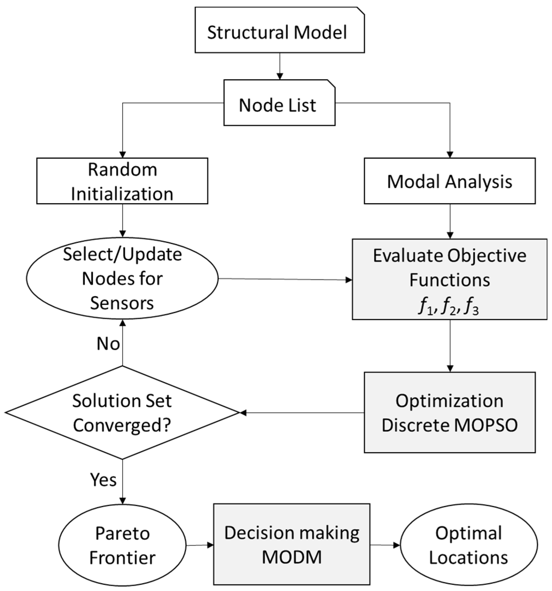
2.1. Optimization Procedure

The basic idea of OSP in SHM is to identify a layout for a certain number of sensors that can be used to obtain as much information as possible regarding a dynamic system. To realize this objective, the first step is to express a full-scale analytical model in finite-element software, such as Abaqus. Through modal analysis, modal properties such as mode shapes and natural frequencies can be calculated. Then, the input parameters for an OSP process are computed and the objective functions are defined. Next, the optimization algorithm is executed, and it returns a Pareto set. Finally, a multiobjective decision-making (MODM) strategy is applied to determine the most feasible solution as the final output OSP. Figure 1 illustrates the process adopted in this study.

When we set the objective function, we considered key factors such as the spatial intersection angle of the modal vector, the redundancy of the collected data, and the intensity of the collected signal. According to Equation (1), the examined MOP has three objective functions, which must be minimized in the exploration space $\Omega$. The goal of optimization is to calculate the feasible solution sets for the objective functions and to return the optimal sensor layout solution in the context of the decision strategy.

$$\mathrm{Minimize} F\left(x\right)=\left\{f_1\left(x\right),f_2\left(x\right),f_3\left(x\right)\right\}, \mathrm{for} x\in \Omega$$

(1)

2.2. Objective Functions

For the OSP problem, the first step is to obtain the mass and stiffness matrices of the model through modal analysis. Then, one can extract the dynamic properties of the structure, which are easy to achieve in a relevant finite-element model. When a large-scale structure is modeled in some FEM program, the model typically has a high number of DOFs, and possible sensor locations can only be selected from a subset of the total DOFs. Friswell et al. [23] proposed an improved iterated reduced system (IIRS) technique to reduce DOFs of a model in an iterative manner. By using the mass and stiffness matrices as input parameters, a transformation matrix can be obtained after certain loops. The convergence of those loops has been proven in [24]. The key point here is that human OSP analysts must manually define some possible elements as master DOFs and manually eliminate slave DOFs. Then, the reduced mass and stiffness matrices can be employed in OSP.

2.2.1. Linear Independency of Mode Shapes

To distinguish the various modes in a modal test, the measured modal vectors of the structure should be as linearly independent as possible. Moreover, to match the identified mode shapes with the modes obtained through finite-element analysis, the modes of the structure must be distinguished. The MAC matrix proposed by Carne and Dohrmann [5] can be used to evaluate the degree of correlation between modes.

$$MA{C}_{i,j}=\frac{{\Phi }_i^T{\Phi }_j}{\sqrt{\left({\Phi }_i^T{\Phi }_i\right)\left({\Phi }_j^T{\Phi }_j\right)}},$$

(2)

where Φ is the mode shape matrix, which is calculated using the reduced order model in this study. The subscripts i and j denote the ith row and jth column of Φ, respectively, which are indicators of the order of the selected modes.

Two of the most commonly used MAC matrix optimization methods were compared in [6]. In this study, we used the least squares method, which minimizes the sum of the off-diagonal-element least squares in the MAC matrix as the first objective function for evaluating the linear independence of modal shapes, as presented in Equation (3).

$$f_1={{\displaystyle \sum }}_{\begin{array}{c}i=1,j=1\\ \left(i\ne j\right)\end{array}}^s{\left(MA{C}_{i,j}\right)}^2,$$

(3)

where s is the total number of selected modes for OSP. The subscripts i and j denote the ith row and jth column of the MAC matrix, respectively.

2.2.2. Dynamic Information Redundancy

To solve the problem of data redundancy, Feng et al. [14] proposed a redundancy function by considering the similarity of the two-node modal vectors collected by sensors and defined the two-node similarity function according to Equation (4) by using the L2-norm operator on the matrix.

$$SI{M}_{i,j}=1-\frac{\parallel {\Phi }_i-{\Phi }_j{\parallel }_2}{\parallel {\Phi }_i{\parallel }_2+\parallel {\Phi }_j{\parallel }_2},$$

(4)

where $SI{M}_{i,j}$ is the similarity degree between the ith and jth sensors. If the mode shape matrices collected by two acceleration sensors have the same direction, the value of $SI{M}_{i,j}$ is 1. If the mode shape vectors collected by two sensors have opposite directions, the value of $SI{M}_{i,j}$ is 0. Thus, the redundancy factor can be calculated as follows:

$${f_2=\parallel SIM-I\parallel }_2,$$

(5)

where I is an identity matrix. The redundancy of the data collected under a certain sensor layout can be determined from the $f_2$ value. If the redundancy of the modal data collected under a certain sensor layout is high, the value of $f_2$ is large.

2.2.3. Vibration Response Strength

Many studies have suggested that a sensor should be placed where the vibration signal energy is strong [7,25]. This arrangement improves the signal-to-noise ratio and provides highly accurate modal parameter recognition results. The concept of the average MKE (AMKE) is introduced in this section. The AMKE of each DOF is obtained by averaging the arithmetic mean of each row of the MKE matrix and then summing up all the nodes.

$$AMK{E}_i=\frac{1}{m}{{\displaystyle \sum }}_{j=1}^{m}MK{E}_{i,j}=\frac{1}{m}{{\displaystyle \sum }}_{j=1}^{m}diag \left({\Phi }_i^T{\Phi }_j\right),$$

(6)

where m denotes the total modes selected to solve the OSP. The higher AMKE is, the better signal quality is. To transform the problem into a minimizing optimization problem, we introduce a third objective function, namely $f_3$, which is defined as the MKE of all nodes divided by that of the sensor-placed nodes. The parameter $f_3$ is expressed as follows:

$$f_3=\frac{{{\displaystyle \sum }}_{i=1}^{n}AMK{E}_i}{{{\displaystyle \sum }}_{i=1}^{s}AMK{E}_i},$$

(7)

where n is the total number of possible locations for OSP and s is the total number of sensors. The numerator is the MKE of all the nodes, which is a constant in this model, and the denominator is the MKE of the sensor-placed nodes; thus, $f_3$ is always greater than or equal to 1. If sensors are appropriately placed to capture vibration signals, the denominator will be larger; hence lower $f_3$ is better.

2.3. Multiobjective Optimization Algorithm

In the basic PSO algorithm, each particle in the swarm learns from Pbest (personal best) and Gbest (global best). Tabu search can be incorporated into PSO to enhance its performance by prohibiting repeated searches [26]. However, OSP is a discrete and combinatorial optimization problem in a finite-element model. Therefore, a discrete decomposition-based multiobjective PSO (DMOPSO) framework is proposed (Figure 2).

2.3.1. Discrete Particle Status

To comply with the discrete representation of nodes in finite-element analysis, we redefine the terms position and velocity used in PSO in a discrete form as follows:

• Position: In PSO, the position vector represents a solution of the optimized problem. For the OSP problem, the position permutation of a particle i is defined as $X_i=\left\{x_1,x_2,\cdots ,x_n\right\}$. Each dimension of position is a random integer $x_i\in \left[1,n\right]$, where n is equal to the total number of DOFs. The positions of all particles pertain to potential sensor nodes; all initial positions are randomly sampled.
• Velocity: The discrete velocity of particle i is defined as $V_i=\left\{v_1,v_2,\cdots ,v_n\right\}$. The parameter $V_i$ is binary-coded. Moreover, if $v_i=1$, the corresponding element $x_i$ in the position vector changes; otherwise, $x_i$ maintains its original state. The initial velocity of the particles is 0.

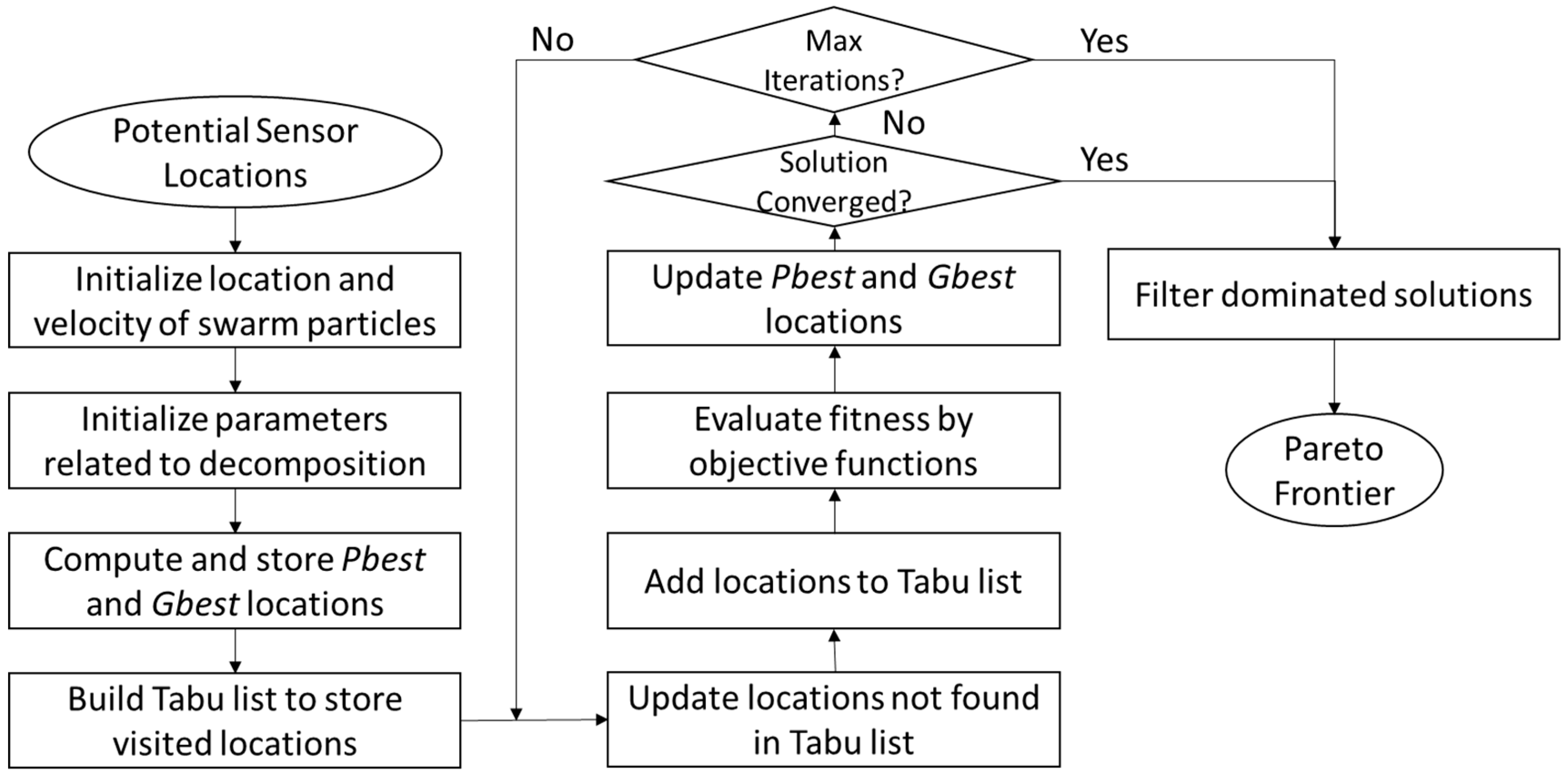
The definition of the position vector is straightforward and easy to decode; thus, it tends to minimize the computational complexity. The aforementioned velocity definition is intended to prevent particles from flying away because setting a threshold $V_{max}$ is generally essential for inhibiting particles from flying outside computational boundaries. However, because our velocity is binary-coded, $V_{max}$ is no longer required. In addition, because the defined position vector is integer-coded, defining a suitable velocity to work on the position is nontrivial. The redefined velocity reflects the differences between two position vectors.

In DMOPSO, a velocity provides a particle with its moving direction and tendency. After updating the velocity, one particle makes use of the new velocity to formalize a new position. Because position and velocity are integer vectors, the mathematical updating rules in continuous PSO no longer require discrete representation. Therefore, we redefine the rules to meet the requirements of our OSP problem. We first redefine the velocity updating rule in discrete form as follows:

$$V_i^{new}=B\left(\omega V_i+c_1{r}_1\left(Pbes{t}_i\oplus X_i\right)+c_2{r}_2\left(Gbes{t}_i\oplus X_i\right)\right),$$

(8)

where $\omega$ is the inertia weight; $c_1$ and $c_2$ are the cognitive and social components, respectively; $r_1$ and $r_2$ are two random numbers in the range of 0–1; and $\oplus$ is the XOR operator. The binary function $B$ is defined as follows:

$$B\left(x_i\right)=\{\begin{array}{c}1, \mathrm{if} rand\left(0,1\right)<sigmoid\left(x_i\right)\\ 0, \mathrm{if} rand\left(0,1\right)\ge sigmoid\left(x_i\right)\end{array},$$

(9)

where the sigmoid function is defined as follows:

$$sigmoid\left(x\right)=\frac{1}{1+e^{-x}}$$

(10)

To promote exploration and exploitation, the inertia weight $\omega$ is randomly generated between 0 and 1. Moreover, the cognitive and social components $c_1$ and $c_2$ are set to the typical value of 1.494, as suggested by [22]. Finally, given a position vector $X$ and velocity vector $V$, we can update the positions according to the newly defined discrete velocity updating rule as follows:

$$x_i^{new}=\{\begin{array}{c}{x}_i,\mathrm{if} v_i=0\\ rand\left({\Omega }_1\right), \mathrm{if} v_i=1\end{array},$$

(11)

where ${\Omega }_1$ represents the position set that has not been visited; that is, the position set that has not been listed in the tabu list.

2.3.2. DMOPSO

Stochastic approaches for solving MOPs usually suffer from high computational complexity. The Penalty Boundary Intersection approach proposed by Zhang and Li [13] decomposes an MOP into numerous subproblems and optimizes each subproblem according to its neighboring subproblems. This utilizes a weighted vector w and penalty value $\theta$ for minimizing the distance to the ideal objective vector $d_1$ and direction error to the weighted vector $d_2$ from the objective function vector $F\left(x\right)$. Therefore, the optimization problem can be expressed using Equation (12), in which d₁ and d₂ are determined using Equation (13).

$$\mathrm{Minimize} g^{pbi}\left(x|w,z\right)=d_1\left(F\left(x\right)|w,\mathrm{z}\right)+\theta d_2\left(F\left(x\right)|w,\mathrm{z}\right)$$

(12)

$$\begin{gathered} d_1\left(f|w,z\right)=\frac{{\parallel \left(f-z\right)}^{T}w\parallel }{\parallel w\parallel } \\ {d}_2\left(f|w,z\right)=\parallel f-\left(z+\frac{d_1}{\parallel w\parallel }w\right)\parallel , \end{gathered}$$

(13)

where z is the ideal point with minimum value in each objective and T is the neighborhood size.

The procedure for OSP in SHM when using the proposed DMOPSO algorithm comprises two major blocks. The initialization block involves the following steps:

• Generate a well-distributed weighted vector ($W={\left\{w^1,\cdots ,w^N\right\}}^T)$.
• Initialize neighborhood N according to the Euclidean distance (i.e.,$N={\left\{n^1,\cdots ,n^N\right\}}^T$, $n^i=\left[n_1,\cdots ,n_T\right])$.
• Set the initial reference point $z^{id}$.
• The personal best position initialization $Pbest={\left\{pbes{t}^1,\cdots ,pbes{t}^N\right\}}^T$, $pbes{t}^i=x^i$.
• Set t = 0.

The loop block involves the following steps when t < MaxIter:

• Randomly select one particle from the neighbors as the Gbest particle.
• Calculate the new position $x_i^{t+1}$.
• Compute the objective function vector F.
• Update the neighborhood solutions. For the jth particle in the neighborhood of the ith particle, $x_i^t=x_i^{t+1}$ if $g^{pbi}\left(x_i^{t+1}|w_j,z\right)\le g^{pbi}\left(x_i^t|w_j,z\right)$.
• Update reference point $z$.
• Update the personal best solution Pbest.
• Set t = t + 1.

2.4. Decision on the Pareto Frontier

After we obtain the Pareto set of the OSP problem, the next step is to determine which solution from the Pareto set can be the final placement. Because no physical relationship exists among the three objective functions, we define a normalization rule to map them to the range between 0 and 1. The membership function $\mu$ is computed as follows:

$$\mu \left(f_{i,j}\right)=exp\left[-{\left(\frac{f_{i,j}-f_j^{}}{\frac{1}{k}{{\displaystyle \sum }}_{i=1}^k\left|f_{i,j}-f_j^{}\right|}\right)}^2\right],$$

(14)

where the subscript i represents the ith solution corresponding to the Pareto set and the subscript j represents the jth objective corresponding to the Pareto set. Thus, $f_{i,j}$ indicates the value of the ith Pareto solution for the jth objective, and $f_j^{}$ indicates the minimum value of the jth objective function among k solutions.

To combine the $\mu$ of each objection function, a weighted square sum rule is used. The ith closeness distance CD_i, which is defined using Equation (15), is an overall performance measure of OSP. Due to the lack of a-priori information regarding the weights of the objective functions, equal weights are assumed to achieve the most balanced solution for each objective. The weightings can be tuned if some practical reasons bias the preference of objective functions. For example, defining the whole weight for $f_1$ reduces to the traditional MAC approach. Or if the structure is subject to noisy environment, a greater weight on $f_3$ is preferred. In this DMOPSO algorithm used in this study, only CD_i is recomputed without influencing the obtained Pareto set.

$$C{D}_i=\sqrt{{{\displaystyle \sum }}_{j=1}^q{w}_j{\mu }_{ij}^2},$$

(15)

where q is the number of objectives (3 in this study). Equation (15) indicates that the solution with the highest CD is selected as the final output OSP result.

3. Validation

3.1. Model Setup

We validated the proposed OSP objective functions by using the DMOPSO algorithm on the Canton Tower, which has a height of 610 m. This building was previously studied by Yi et al. [27,28] and Sun et al. [6]. The method proposed in this paper was compared with the Immune Monkey Algorithm presented in [26] and the discrete Artificial Bee Colony algorithm presented in [6]. Canton Tower comprises two parts, namely a 454-m-high main tower and 156-m-high steel antenna mast. The main tower is a tube-in-tube structure consisting of a steel lattice outer structure and reinforced concrete inner structure. Detailed descriptions and photos of this structure can be found in [28]. The present study extended a preliminary study on FEM analysis and a simplified 3D beam model with lumped mass that was proposed by Ni et al. [29]. The simplified model consisted of 37 beam elements, with 27 elements for the main tower and 10 elements for the antenna mast. Each beam node had five DOFs (two horizontal translations and three rotations) when neglecting the vertical deformation. Therefore, the beam model comprised 185 DOFs. As in previous studies, we only considered the horizontal translation DOFs for OSP. We applied the IIRS technique to the open-access data provided by Ni [29] to reduce the 3D beam model. Consequently, a reduced model that only considers horizontal translation DOFs was obtained. The obtained reduced model had 74 DOFs, which were considered as candidate sensor locations. This part of the present study is the same as the work presented in [6,27,28] for a fair comparison of the same model. We used the same settings (e.g., the number of sensors) for the OSP framework and proposed MODM strategy.

Given the stiffness and mass matrices of the aforementioned finite-element model of Canton Tower, the mode shape matrix $\Phi$ was computed. The optimization algorithm was then implemented in MATLAB, and the order of modes m (=15) as well as the number of sensors s (=20) were fed into the algorithm, whose parameters were configured as follows:

PSO: Particle swarm population size N = 210 and maximum iteration cycle MaxIter = 1000.

DMOPSO: Neighborhood size T = 21; number of subobjectives = 210 (equal to the population size); number of solution sets on the Pareto front = 100; and decomposition penalty value $\theta$ = 5.

3.2. Results

Table 1. Results of 33 independent runs with the proposed method and the membership function values in the Pareto set for each run. The values higher than the average value of the corresponding objective function are highlighted in bold; and the superior results for the three objectives presented against a gray background.

Set No.	Objective Function			Membership Function
	f1	f2	f3	${\mu }_1$	${\mu }_2$	${\mu }_3$	CD
1	4.2023	6.4217	1.9346	0.9855	0.0039	0.9974	1.4022
2	3.2291	6.9469	2.0654	0.9959	0.0001	0.9749	1.3937
3	3.2291	6.9469	2.0654	0.9959	0.0001	0.9749	1.3937
4	3.2291	6.9469	2.0654	0.9959	0.0001	0.9749	1.3937
5	3.2932	7.0005	1.9632	0.9964	0.0003	0.9943	1.4077
6	2.9205	6.9322	2.1283	0.9991	0.0013	0.9644	1.3886
7	3.7596	7.0590	2.0437	0.9921	0.0010	0.9854	1.3983
8	3.2291	6.9469	2.0654	0.9959	0.0001	0.9749	1.3937
9	3.2932	7.0005	1.9632	0.9964	0.0003	0.9943	1.4077
10	3.3699	8.1701	1.9502	0.9959	0.0000	0.9987	1.4104
11	3.8235	7.0973	1.9064	0.9911	0.0005	0.9972	1.4060
12	3.2932	7.0005	1.9632	0.9964	0.0003	0.9943	1.4077
13	3.3699	8.1701	1.9502	0.9959	0.0000	0.9987	1.4104
14	3.7296	6.7387	1.9861	0.9917	0.0076	0.9984	1.4073
15	3.5830	6.7788	1.9682	0.9927	0.0008	0.9957	1.4060
16	3.3699	8.1701	1.9502	0.9959	0.0000	0.9987	1.4104
17	2.8888	7.2074	2.1425	0.9991	0.0000	0.9692	1.3920
18	3.2932	7.0005	1.9632	0.9964	0.0003	0.9943	1.4077
19	3.7296	6.7387	1.9861	0.9917	0.0076	0.9984	1.4073
20	3.8045	6.8785	1.9493	0.9899	0.0006	0.9997	1.4069
21	3.4290	7.5629	1.9786	0.9954	0.0000	0.9935	1.4063
22	3.1451	7.2698	2.0283	0.9978	0.0006	0.9874	1.4038
23	3.8045	6.8785	1.9493	0.9899	0.0006	0.9997	1.4069
24	3.5403	7.7830	1.8722	0.9949	0.0000	0.9984	1.4093
25	3.7296	6.7387	1.9861	0.9917	0.0076	0.9984	1.4073
26	3.1596	7.8314	1.8752	0.9973	0.0002	0.9957	1.4093
27	3.3179	7.3410	2.0130	0.9971	0.0002	0.9938	1.4078
28	3.1799	6.7150	1.9181	0.9934	0.0010	0.9988	1.4087
29	3.1451	7.2698	2.0283	0.9978	0.0006	0.9874	1.4038
30	3.3699	8.1701	1.9502	0.9959	0.0000	0.9987	1.4104
31	3.8045	6.8785	1.9493	0.9899	0.0006	0.9997	1.4069
32	3.5207	7.1577	1.9210	0.9926	0.0003	1.0000	1.4090
33	3.0762	7.0062	2.0031	0.9987	0.0011	0.9883	1.4051
Mean	3.4196	7.1525	1.9843	0.9946	0.0011	0.9915	1.4044

presents the 33 solution sets obtained from independent OSP runs with 20 sensors. The objective function value and the membership value of the final optimal solution obtained in each run were notably close. An observation of the membership value indicates that the best solution obtained is the solution with the highest ranking in the corresponding solution set for $f_1$ and $f_3$. Moreover, the solution obtained for $f_2$ is notably poor in the solution set. Thus, among the three set targets, all the solutions that stand out through the set conditions conform to a loose rule, that is, the nondiagonal elements of the measured signal MAC matrix are minimized to maintain the linear vibration of the mode shape. The signal strength of the vibration response can provide a relatively accurate solution; however, the redundancy in the acquisition signal is poor. Thus, the three indicators are completely independent and have no influence on each other. This finding proves that no abnormal solution exists in the multiobjective optimization and decision-making results, which indicates that the optimization program is correct and the decision-making process is robust.

Table 1 presents the dominant solution sets within the complete set of solution sets. The values higher than the average value of the corresponding objective function are highlighted in bold. Moreover, superior results for the three objectives are presented against a gray background. Regarding the averages of the 33 solution sets, the bold numbers were less than the average of the target Pareto solution set (Set Nos. 5, 9, 12, and 18). The results of Set No. 28 were smaller than the average value for all the objectives. Moreover, the results of Set No. 5 were larger than those of Set No. 28 for all the objectives, which indicated that Set No. 5 was dominated by Set No. 28. Figure 3 presents the visualizations of Pareto Set No. 28 from different dimensions. Because Solution No. 28 outperformed the other solutions, we compared Solution No. 28 with the solutions of other OSP methods from the literature.

3.3. Discussion

Table 2. Optimal sensor placement (OSP) node ID of the Canton Tower when using 20 sensors with different methods.

Direction	MOP-No. 28	Reference [27]	Reference [6] (o.1)	Reference [6] (o.2)
x	5, 6, 10, 14, 16, 17, 22, 25, 26, 27	2, 6, 14, 20, 21, 22, 23, 24, 29	2, 3, 17, 18, 19, 20, 21, 22, 23	1, 2, 3, 4, 5, 14, 18, 19, 20, 21, 26
y	3, 4, 9, 11, 16, 20, 22, 25, 26, 27	1, 2, 4, 5, 6, 7, 11, 16, 20, 22, 23	1, 2, 3, 10, 17, 19, 20, 21, 22, 24, 28	3, 4, 5, 8, 17, 19, 20, 23, 27

presents the OSP results obtained for the Canton Tower when using different approaches. The results from referenced papers are referred to with square brackets, followed by denotation to separate variants. References [27] and Reference [6] (o.1) used the same optimization objective to minimize the maximum off-diagonal element. The difference between the aforementioned references is related to the algorithm used for optimization. References [6] (o.1) and [6] (o.2) used the same algorithm for optimization, but Reference [6] (o.2) minimized the sum of the least squares of the off-diagonal elements; thus, Reference [6] (o.2) used the first objective function in this study.

We added the different OSP solutions into the proposed objective function to compare values.

Table 3. Comparison of the solutions obtained with different methods when using the proposed objective function and closeness.

Method	f1	f2	f3	${\mu }_1$	${\mu }_2$	${\mu }_3$	CD
MOP-No. 28	3.1799	6.7150	1.9181	0.9934	0.0001	0.9624	1.4087
Reference [27]	6.8546	6.1141	3.1888	-	-	-	-
Reference [6] (o.1)	4.7892	7.6955	2.7343	-	-	-	-
Reference [6] (o.2)	2.1766	6.0536	1.9181	1.0000	0.0247	0.6191	1.1764

indicates that the method of minimizing the maximum off-diagonal elements has no obvious advantages over the method used in [6] (o.2) and the MOP. The results of the aforementioned solutions exhibit poor performance for $f_2$; thus, the results have no comparative significance. The results of the single-objective optimization method used in [6] (o.2) are superior to those of the MOP method for $f_1$. By contrast, for $f_3$, the solution of the MOP method is superior to that of the single-objective method.

We subsequently calculated the two solution groups for Pareto Set No. 28 simultaneously with the proposed MODM method. We used MODM analysis to compare the performance levels of the MOP method and the method used in [6] (o.2). The membership functions and closeness distance of [6] (o.2) indicated that its solution was inferior to that of the MOP method. For the first objective, the single-objective algorithm exhibited the best performance, which is in line with the expectation. Thus, the multiobjective optimization algorithm still has room for progress in single-objective convergence. The membership values in Table 3 indicate that the multiobjective optimization solution in the first and third objectives were notably close to the results of the ideal solution in the solution set. Moreover, the method used in [6] (o.2) provided the best results for the first objective; however, this method only provided average results for the third objective. Thus, the MOP method outperformed the method in [6] (o.2) for the third objective. The results also indicated that the aforementioned two optimization methods were not effective for the second objective.

4. Application

4.1. Model Setup

To further test the effectiveness of OSP in SHM for complex structures, we conducted an experiment on a three-story aluminum frame structure, illustrated in Figure 4a with a 50 cm ruler for scale, as an attempt to mimic offshore jacket structures. The structure was composed of four square frames and four slanted legs. The sides of the square structure had dimensions of 0.5, 0.45, 0.4, and 0.35 m from bottom to top. The spacing of each layer from bottom to top was 0.5 m; thus, the height of the structure was 1.5 m. The material used was aluminum, and all joints were connected with bolts. The frame was constructed with an angle section profile (25 × 25 × 2 mm³). The bottom layer was fixed on an optical table to prevent horizontal motion and vibration. The mechanical properties of aluminum are as follows: Young’s modulus = 68.9 GPa, Poisson’s ratio = 0.33, and density = 2850 kg/m³.

A corresponding finite-element model was developed for OSP, as illustrated in Figure 4b,c. The model had 232 nodes, 244 beam elements, and 1176 DOFs. The same angle section profile was applied on all elements. Modal analysis was performed with fixed constraints at the four bottom corners. Because the structure was vertically symmetrical, its natural frequencies were expected to be the same in horizontal directions. At the beginning of modal analysis, by using the IIRS technique, only 70 translational DOFs (along the x-direction and y-direction) were considered for OSP. The results of modal analysis were fed to an optimization process, which output the eight most effective locations for sensors. MOP optimization was conducted for the same configuration as that of Canton Tower to determine the optimal locations for sensors. In addition, we used the traditional forward sequential sensor placement (FSSP) algorithm [7] to discover different optimization solutions. The FSSP algorithm minimizes the sum of the least squares of the off-diagonal elements of a MAC matrix (i.e., the objective is MinMAC). The third method involved random placement by excluding the nodes selected by the FSSP algorithm.

A vibration test was then performed on the physical model. The structure was instrumented with eight single-axis accelerometers. The OSP locations were obtained using the MOP, FSSP, and random placement methods. Four sensors were oriented in the x-direction, and the other four were oriented in the y-direction. A random impulse signal was applied at the upper corner of the frame (Node 29) on the structure along the y-direction. The sample rate of data acquisition was 25,600 Hz, and data were recorded for 10 s. The modal properties of the structure were identified using frequency domain decomposition on the basis of all the nodal measurements. Then, vibration signals were processed to obtain the power spectral density (PSD) matrix. The vibration signals were also compared with modal frequencies from FEM analysis. Moreover, the relative displacements between sensors were computed at the first six modal frequencies to obtain a mode shape matrix for calculating objective functions. Because we did not measure all the nodes for potential sensor locations, $f_3$ could not be calculated. We slightly modified Equation (7) by setting the AMKE obtained from the MOP method as the reference value, which was divided by the AMKE obtained from other methods, as per Equation (16). If the value obtained after the aforementioned division was greater than 1, the results of this sensor placement method were worse than those of the MOP method for $f_3$.

$$f_3=\frac{{{\displaystyle \sum }}_{i=1}^{s}AMK{E}_i{}^{MOP}}{{{\displaystyle \sum }}_{i=1}^{s}AMK{E}_i},$$

(16)

4.2. Result and Discussion

The modal analysis of the finite-element model provided the modal frequencies and corresponding mode shapes. The first 10 modes are listed in

Table 4. Modal frequencies in Hz.

Mode	FEM	EXP (MOP)	Error
1	20.957	18	−14%
2	20.957	18	−14%
3	27.896	22	−21%
4	64.043	54	−16%
5	64.043	55	−14%
6	88.013	70	−20%
7	105.76	96	−9%
8	113.89	103	−10%
9	113.89	104	−9%
10	134.46	119	−11%

, and the first six mode shapes are illustrated in Figure 5. Due to the symmetry of the model, mode frequencies (1, 2), (4, 5), and (8, 9) were exactly paired, and the mode shapes were the same in horizontal directions. The modal frequencies predicted by FEM are systematically higher than those obtained from the experiment. A possible reason is due to the presence of the bolt joints for the physical model, which is absent for the finite-element model. The presence of bolt joints added additional weight to the structure and also reduced flexural stiffnesses of the structural members, both potentially resulting in lower modal frequencies of the entire structure.

Subsequently, the FEM results were input into OSP algorithms, which output the eight best locations, as listed in

Table 5. Sensor placement and performance evaluation for the three OSP methods.

Method	X-Direction	Y-Direction	f1	f2	f3
MOP	5, 16, 25, 31	6, 15, 25, 34	0.2633	1.8006	1
FSSP	7, 12, 26, 28	4, 6, 18, 22	0.1475	1.9335	2.2136
Random	11, 19, 23, 31	5, 9, 17, 21	0.4197	2.7686	0.9078

. The sensor positions obtained using three methods are illustrated in Figure 6, where Node 29 is the excitation node, green arrows represent x-direction sensors, and magenta arrows represent y-direction sensors. Node 25 in the MOP method was collocated by two sensors, which were not limited by the MOP algorithm. These sensors were placed on the selected nodes of the physical model according to Table 5, and we performed vibration tests for each selection.

Figure 7 illustrates the acceleration PSDs of each sensor when using the MOP method. This figure spans a frequency range from 0 to 130 Hz, which covers the first 10 modes of the frame structure. Note that the PSD of No. 8 sensor at Node 34 shows the greatest amplitude and cleanest signals among the eight deployed sensors. The primary reason is attributed to the nature of the operational modal analysis method in the present study when performing singular value decomposition for identifying the PSDs. Either the sensor location near the free ends or close to excitation node may also affect the signal amplitudes, but is of secondary importance. Nevertheless, only peak frequencies without the need of signal amplitude of the PSDs are of interest for determining the modal frequencies. The peak frequencies are obtained (See examples indicated by the pink-dashed vertical lines in the PSDs of No. 2 and 6 sensors) and listed in Table 4, and compared with the values predicted using the FEM. The symmetry of modes was also resolved; however, the frequencies were on average 14% lower than those obtained through the FEM. The signals from different sensors did not indicate significant differences in modal frequencies. In terms of the characteristics of frequency response, the modes along the x-direction and the torsional modes were well excited. Distinctive peaks were observed, which proved that rich structural information was included in the measurements at the OSP locations.

The signals were further processed to evaluate the mode shape matrices of sensing DOFs through singular value decomposition. Three objective functions were computed with their corresponding matrices (Table 5). The best result for $f_1$ was obtained with the FSSP method because MinMAC was the only objective in FSSP. For the other two objectives, the MOP method outperformed the FSSP method. Surprisingly, the random placement method achieved optimal performance for $f_3$; however, for $f_1$ and $f_2$, its performance levels were notably inferior to those of the other two methods. Because $f_1$ and $f_3$ had a negative correlation, the MOP method provided the most balanced performance for opposing objectives because equal weight was assumed for each objective.

5. Conclusions

We developed a decomposition-based multiobjective PSO algorithm with a redefined integer reproduction operator for denoting possible sensor locations in a structure. Three objective functions were defined, linear independence of mode shapes, limited dynamic information redundancy, and maximum vibration response signal strength, for evaluating the performance of sensor placements. Once a Pareto solution set is obtained, a closeness-based MODM strategy was applied to determine the final solution.

Numerical examples were investigated to test the applicability of the proposed MOP framework for OSP. The Canton Tower case was compared with those obtained from two previous studies. The results proved that the proposed method can obtain the optimal values for MAC and MKE metrics; however, it exhibited poor performance in the similarity degree objective. We then tested a more complex frame structure experimentally. Again, the results proved the effectiveness of the proposed algorithm. The test data verified that the experimental and numerical conclusions were consistent. In this case, the MOP approach under the setup of equal-weighting on each objective may not reach the optimal solution in a certain single objective; however, it can discover a notably feasible and balanced solution among contradicting functions. We look forward to SHM applications of various structures and damage detection based on efficient sensor layout obtained with the proposed OSP algorithm.

References

1. Kammer, D.C. Sensor placement for on-orbit modal identification and correlation of large space structures. J. Guid. Control Dyn. 1991, 14, 251–259. [Google Scholar] [CrossRef]
2. Heo, G.; Wang, M.; Satpathi, D. Optimal transducer placement for health monitoring of long span bridge. Soil Dyn. Earthq. Eng. 1997, 16, 495–502. [Google Scholar] [CrossRef]
3. Papadimitriou, C. Optimal sensor placement methodology for parametric identification of structural systems. J. Sound Vib. 2004, 278, 923–947. [Google Scholar] [CrossRef]
4. Ewins, D.J.; Saunders, H. Modal Testing: Theory and Practice. J. Vib. Acoust. 1986, 108, 109–110. [Google Scholar] [CrossRef]
5. Carne, T.G.; Dohrmann, C.R. A Modal Test Design Strategy for Model Correlation; Sandia National Labs: Albuquerque, NM, USA, 1994.
6. Sun, H.; Büyüköztürk, O. Optimal sensor placement in structural health monitoring using discrete optimization. Smart Mater. Struct. 2015, 24, 125034. [Google Scholar] [CrossRef]
7. Ostachowicz, W.; Soman, R.; Malinowski, P. Optimization of sensor placement for structural health monitoring: A review. Struct. Health Monit. 2019, 18, 963–988. [Google Scholar] [CrossRef]
8. Deb, K.; Jain, H. An Evolutionary Many-Objective Optimization Algorithm Using Reference-Point-Based Nondominated Sorting Approach, Part I: Solving Problems with Box Constraints. IEEE Trans. Evol. Comput. 2013, 18, 577–601. [Google Scholar] [CrossRef]
9. Yang, S.; Li, M.; Liu, X.; Zheng, J. A Grid-Based Evolutionary Algorithm for Many-Objective Optimization. IEEE Trans. Evol. Comput. 2013, 17, 721–736. [Google Scholar] [CrossRef]
10. Wang, R.; Purshouse, R.C.; Fleming, P.J. Preference-inspired coevolutionary algorithms for many-objective optimization. IEEE Trans. Evol. Comput. 2013, 17, 474–494. [Google Scholar] [CrossRef]
11. Cheng, R.; Jin, Y.; Olhofer, M.; Sendhoff, B. A Reference Vector Guided Evolutionary Algorithm for Many-Objective Optimization. IEEE Trans. Evol. Comput. 2016, 20, 773–791. [Google Scholar] [CrossRef] [Green Version]
12. Bader, J.; Zitzler, E. HypE: An Algorithm for Fast Hypervolume-Based Many-Objective Optimization. Evol. Comput. 2011, 19, 45–76. [Google Scholar] [CrossRef] [PubMed]
13. Zhang, Q.; Li, H. MOEA/D: A Multiobjective Evolutionary Algorithm Based on Decomposition. IEEE Trans. Evol. Comput. 2007, 11, 712–731. [Google Scholar] [CrossRef]
14. Feng, S.; Jia, J. Acceleration sensor placement technique for vibration test in structural health monitoring using microhabitat frog-leaping algorithm. Struct. Health Monit. 2017, 17, 169–184. [Google Scholar] [CrossRef]
15. Guo, Y.; Ni, Y.; Chen, S. Optimal sensor placement for damage detection of bridges subject to ship collision. Struct. Control Health Monit. 2016, 24, e1963. [Google Scholar] [CrossRef]
16. Lin, J.-F.; Xu, Y.; Law, S.-S. Structural damage detection-oriented multi-type sensor placement with multi-objective optimization. J. Sound Vib. 2018, 422, 568–589. [Google Scholar] [CrossRef]
17. Kennedy, J.; Eberhart, R.C. A discrete binary version of the particle swarm algorithm. In Proceedings of the 1997 IEEE International Conference on Systems, Man, and Cybernetics. Computational Cybernetics and Simulation, Orlando, FL, USA, 12–15 October 1997; Volume 5, pp. 4104–4108. [Google Scholar]
18. Coello, C.; Pulido, G.; Lechuga, M. Handling multiple objectives with particle swarm optimization. IEEE Trans. Evol. Comput. 2004, 8, 256–279. [Google Scholar] [CrossRef]
19. Nebro, A.; Durillo, J.; Garcia-Nieto, J.; Coello, C.C.; Luna, F.; Alba, E. SMPSO: A new PSO-based metaheuristic for multi-objective optimization. In Proceedings of the 2009 IEEE Symposium on Computational Intelligence in Multi-Criteria Decision-Making, Nashville, TN, USA, 30 March–2 April 2009; pp. 66–73. [Google Scholar]
20. Al Moubayed, N.; Petrovski, A.; McCall, J. D2MOPSO: MOPSO Based on Decomposition and Dominance with Archiving Using Crowding Distance in Objective and Solution Spaces. Evol. Comput. 2014, 22, 47–77. [Google Scholar] [CrossRef] [Green Version]
21. Lin, Q.; Li, J.; Du, Z.; Chen, J.; Ming, Z. A novel multi-objective particle swarm optimization with multiple search strategies. Eur. J. Oper. Res. 2015, 247, 732–744. [Google Scholar] [CrossRef]
22. Gong, M.; Cai, Q.; Chen, X.; Ma, L. Complex Network Clustering by Multiobjective Discrete Particle Swarm Optimization Based on Decomposition. IEEE Trans. Evol. Comput. 2013, 18, 82–97. [Google Scholar] [CrossRef]
23. Friswell, M.; Garvey, S.; Penny, J. Model reduction using dynamic and iterated IRS techniques. J. Sound Vib. 1995, 186, 311–323. [Google Scholar] [CrossRef]
24. Friswell, M.; Garvey, S.; Penny, J. The convergence of the iterated IRS method. J. Sound Vib. 1998, 211, 123–132. [Google Scholar] [CrossRef]
25. Li, D.-S.; Li, H.; Fritzen, C. The connection between effective independence and modal kinetic energy methods for sensor placement. J. Sound Vib. 2007, 305, 945–955. [Google Scholar] [CrossRef]
26. Behera, S.; Sahoo, S.; Pati, B. A review on optimization algorithms and application to wind energy integration to grid. Renew. Sustain. Energy Rev. 2015, 48, 214–227. [Google Scholar] [CrossRef]
27. Yi, T.-H.; Li, H.-N.; Zhang, X.-D. Health monitoring sensor placement optimization for Canton Tower using immune monkey algorithm. Struct. Control Health Monit. 2014, 22, 123–138. [Google Scholar] [CrossRef]
28. Yi, T.-H.; Li, H.-N.; Zhang, X.-D. Sensor placement on Canton Tower for health monitoring using asynchronous-climb monkey algorithm. Smart Mater. Struct. 2012, 21. [Google Scholar] [CrossRef]
29. Ni, Y.; Xia, Y.; Lin, W.; Chen, W.; Ko, J. SHM benchmark for high-rise structures: A reduced-order finite element model and field measurement data. Smart Struct. Syst. 2012, 10, 411–426. [Google Scholar] [CrossRef] [Green Version]
Figure 1. Flowchart of proposed method.
Applsci 10 07710 g001
Figure 2. Flowchart of the discrete decomposition-based multiobjective particle swarm optimization (DMOPSO) algorithm.
Applsci 10 07710 g002
Figure 3. Visualization of Pareto Set No. 28: (a) Three objectives; (b) visualization of f 1 and f 2 ; (c) visualization of f 1 and f 3 ; and (d) visualization of f 2 and f 3 .
Applsci 10 07710 g003
Figure 4. Three-story two-bay experimental frame structure: (a) Physical model, (b) finite-element model with sectional profile rendering, and (c) finite-element mesh with nodes (red dots) and fixed boundary conditions (white triangles).
Applsci 10 07710 g004
Figure 5. First six modes of the frame structure computed through the FEM.
Applsci 10 07710 g005
Figure 6. Three different OSP results along the x- and y-directions: The (a) multiobjective optimization problem (MOP); (b) forward sequential sensor placement (FSSP); and (c) random placement methods.
Applsci 10 07710 g006
Figure 7. Experimental frequency responses of some typical OSP nodes in the MOP results.
Applsci 10 07710 g007