Identification of Unstable Subsurface Rock Structure Using Ground Penetrating Radar: An EEMD-Based Processing Method


1
Department of Structure Engineering, Delft University of Technology, Postbus 5, 2600 AA Delft, The Netherlands
2
Department of Hydraulic Engineering, Tsinghua University, Beijing 100084, China
*
Author to whom correspondence should be addressed.
Appl. Sci. 2020, 10(23), 8499; https://doi.org/10.3390/app10238499
Submission received: 12 October 2020
/
Revised: 23 November 2020
/
Accepted: 25 November 2020
/
Published: 28 November 2020
(This article belongs to the Special Issue Nondestructive Testing (NDT): Volume II)
Abstract
:Featured Application
The approach for extracting features from GPR radargrams was developed based on EEMD. The proposed method was utilized to eliminate the interference signals and reconstruct subsurface profiles. This radargram interpretation approach was applied to identify surrounding cracked rocks of underground caverns.
Abstract
Surrounding rock quality of underground caverns is crucial to structural safety and stability in geological engineering. Classic measures for rock quality investigation are destructive and time consuming, and therefore technology evolution for efficiently evaluating rock quality is significantly required. In this paper, the non-destructive technology ground penetrating radar (GPR) assisted by an ensemble empirical mode decomposition (EEMD)-based signal processing approach is investigated for identifying unstable subsurface rock structures. By decomposing the pre-processed GPR signals into multiple intrinsic mode functions (IMFs) and residues, one typical IMF can preserve the distinct local modes and is considered to reconstruct the subterranean profile. Promising results have been achieved in simple scenarios and filed measurements. The reconstructed profiles can accurately illustrate the subsurface interfaces and eliminate the interference signals. Unstable rock structures have been identified in further field applications. Therefore, the developed approach is efficient in unstable rock structure identification.
1. Introduction
With the rapid development of underground spaces for energy storage [1], transport [2] and mining [3], the surrounding rock stability is increasingly significant for the safe operation of underground caverns. Rock formation can fundamentally determine the geological strength [4], as cracked surrounding rocks risk collapse and require rock reinforcement approaches. To visibly evaluate the surrounding rock quality, opening and pit sampling approaches (e.g., [5,6]) are extensively utilized and can accurately quantify the attribute parameters. However, intermittent sampling fails to detect the entire rock section continuously, while mechanically opening the rocks is destructive and time-consuming. Some researches (e.g., [7,8]) established sensor arrays for stress-strain monitoring, but the detection positions were discontinuously distributed inside the shallow ground. Therefore, developing a field-efficacious non-destructive detection technology to scan the surrounding rock profiles continuously is significant for rock structural stability.
Ground penetrating radar (GPR) is a remote sensing technology originally designed to detect the ice thickness while primarily applied in discovering the unseen objects beneath the earth’s surface, e.g., with applications in mapping subsurface stratigraphy [9], archaeological prospection [10] and detecting pavement defects [11]. Since GPR works as an echo-listener recording electromagnetic waves reflected from interfaces with dielectric differences, this non-destructive technology has the potential to distinguish fresh and weathered rock masses. However, signal interference is an unavoidable issue affecting radargram interpretation. Inversion and migration approaches (e.g., [12,13]) were developed based on Maxwell’s equations to eliminate signal interference, but excessive derivative and integral calculations are time-consuming. Machine learning (e.g., [14,15]) provides automatic approaches for target identification from radargrams, but required considerable datasets with similar underground attributes are difficult to acquire from field measurement. Jin and Duan [16] developed a discrete grid method to eliminate hyperbolic interference in rock detection, but with many parameters determined by experience. Since electromagnetic waves would be reflected and interfered frequently in cracked rock sections, a novel approach is required to improve efficiency in handling signal interference.
Modal analysis is a common signal analysis approach in structural health monitoring. Generally, it characterizes the vibration signals in frequency and time domains, which provide attribute and stability information of the tested structure. The modal difference exists between intact and cracked rock masses, and GPR can capture this subterranean structural feature. Different from classic approaches that concern the physics of wave propagation for GPR signal processing, modal analysis methods consider the physics of signal strength and frequencies. Some researches have attempted to interpret radargrams with these methods, e.g., wavelet transform [17,18] and empirical mode decomposition [19,20], but their applications are either at the de-noise stage or in simple object identification. To our best knowledge, no research has modally analyzed GPR radargrams with complicated targets like cracked rock masses. In the cracked subsurface area, numerous rock fissures are nearly continuously distributed, therefore instantaneous changes of GPR signals becoming significant in modal analysis. Empirical mode decomposition (EMD) was originally proposed by Huang et al. [21] for nonlinear and non-stationary signal analysis and then extensively applied to extract modes from signals (e.g., [22,23]). It can decompose signals into multiple intrinsic mode functions (IMFs) which focus on the local time scale and contain instantaneous frequency information, thereby having the potential to analyze instantaneous changes in radargrams. The decomposition results correspond to the natural mode determined by the signal itself, different from wavelet transform that acquires modes inside certain filter bands. Mode mixing sometimes appears and reduces the decomposition effectiveness, and in order to overcome this disadvantage, ensemble empirical mode decomposition (EEMD) was developed utilizing a white-noise-assisted method [24].
In this paper, an EEMD-based approach is developed to analyze GPR data for the novel application in identifying unstable subsurface rock structures. The remainder of this paper is organized as follows: Section 2 introduces the developed signal processing approach for interpreting GPR radargrams; Section 3 presents the results of both numerically simulated and field-measured GPR signals; Section 4 discusses and concludes this paper.
2. Materials and Methods
2.1. Pre-Processing of GPR Data
To prepare GPR signals well for further EEMD analysis, three significant steps are utilized to pre-process original GPR data: time-depth conversion, ‘de-wow’ and amplitude gain.
Firstly, the time-depth conversion is designed to extract location information from the recorded time series. According to propagation velocity invariant assumption and two-way travelling time (transmission and reflection) of electromagnetic waves in the subterranean area, the recorded depth of interfaces can be determined [25]:
where, v is the propagation velocity of electromagnetic waves, t is the two-way travelling time, c represents the propagation velocity in the vacuum, is the relative magnetic permeability, and is the relative permittivity.
Secondly, ‘de-wow’ processing is utilized to eliminate low-frequency distortions resulting from the inductive coupling effect or early saturation [25]. An effective approach with good practice to handle the ‘wow’ issue is simply removing the average amplitude from the signals [26]:
where, N is the number of discrete signal points, represents the original signal amplitude, and represents the processed signal.
Thirdly, amplitude gain is utilized to amplify the signals against energy loss including propagation attenuation and geological spreading loss [25]. Considering both exponential attenuation and evenly distributed rock fissures, radar signals can be recovered to realistic levels by multiplying Equation (3) [16].
where, is the exponential attenuation parameter, is the geological spreading loss parameter, and is the starting depth for amplitude gain.
2.2. Ensemble Empirical Mode Decomposition
In 1998, Huang et al. [21] proposed EMD for Hilbert transform with physical meanings to analyze nonlinear and non-stationary signals in multiple resolutions. It offers a self-adaptive approach to decompose any complicated signal series into a finite number of IMFs, which focus on the local time scale and involve only one oscillation mode in each waveform. The instantaneous frequency defined in an IMF corresponds well with the local physics of the studied system, which would have an expected performance in interpreting short-distance features from GPR radargrams.
According to the definition, an arbitrary signal and its Hilbert transform form the complex conjugate pair to obtain the analytical signal .
where, i represents the imaginary unit, is the signal amplitude, and is the signal phase. Therefore, the instantaneous frequency is defined as:
In order to handle the issue that the instantaneous frequency has no precise calculation approach, signal data are limited by narrow bands to provide physical meanings for the instantaneous frequency, and these narrow bands can be obtained by EMD procedure.
Processing a single signal series, the EMD method applies the following procedures:
- Firstly record the initial data, , and initialize from , ;
- Find the upper and lower envelopes () of the data by cubic spline interpolation and then calculate their means, ;
- Setting , obtain the rest part by removing the means , , ;
- Repeat the procedure ii. and iii. until satisfies the decomposition threshold, and we can obtain the IMF as . In Huang’s method, the threshold parameter should be between 0.2 and 0.3;
- , calculate the rest part of signals . Repeat the above steps ii. to iv. to obtain diverse IMFs and the final residue data .
After the EMD algorithm, the analytical signal for Hilbert transform with physical meanings is expressed as:
However, the significant drawback of EMD, mode mixing appearing frequently, has depressed its performance and restricted the applications. This effect either mingles signals of widely disparate scales in an IMF, or residents similar-scale signals in different IMFs. A noise assisted method, EEMD, was then developed by Wu and Huang [24] to overcome the problem of mode mixing. In the EEMD approach, the true IMFs are defined as the ensemble mean of multiple decomposition trials, each with initialized data of the original signals plus a random white noise with narrow amplitude, and this thereby improves mode separating as other researches demonstrate [27,28].
The EEMD algorithm can be summarized as follows:
- Initializing from , generate a random white noise and add it to pre-processed signals, . The standard deviation of noise amplitudes is suggested to be 1/5 that of the signals;
- Apply EMD to decompose into different IMFs ;
- , repeat the above two steps for N times, with the minimum value of N should satisfy Equation (9), where is the final standard deviation of error arising from added noises, and is the standard deviation of noise amplitude;
- Obtain the true decomposition results by calculating the ensemble means of all corresponding IMFs.
In our signal processing procedures, EEMD is employed to extract the distinct mode which should arise from fissures or other shattered rock interfaces. Figure 1 shows representative GPR signals from two measurement traces with and without buried objects beneath respectively and their fast Fourier transform results. The distinct mode appears visibly around the depth of buried objects (0.6–0.8 m), which would be evident local modal features for IMFs to capture.
The algorithm for processing GPR data utilizing EEMD is developed:
- Pre-process GPR profiles using time-depth conversion, ‘de-wow’ and amplitude gain;
- Initializing from , obtain the vertical signal series from a single measurement trace , where is the abscissa of the measurement point;
- Apply EEMD to decompose into different IMFs, and preserve the IMF that can distinguish the mode of abnormal objects;
- , repeat the above two steps to process the vertical signals from all measurement traces, and then we can reconstruct the final analytical subterranean profile by all preserved IMFs.
3. Results
3.1. Investigation in Simple Scenarios
The basic approach for identifying the unstable rock structures is to identify the rock interfaces, which is firstly investigated in this paper. Two simple scenarios, a practical radargram with buried objects and a numerically simulated radargram with predefined cracked rock areas, are under investigation to evaluate the accuracy of the developed signal processing approach in locating object interfaces.
Firstly, GPR acquired the subterranean profile with two pre-buried pipelines (32 cm diameters), which are sparsely distributed with around 2.5 m interval. The pipelines are discernible enough and will not interfere each other’s signals because of the large burying distance. The central frequency of GPR attenna is 700 MHz. Figure 2 illustrates the pre-processed radargram, with the measurement length L ( m) and detection depth Z ( m). The pre-processing parameters are , and = 0.25 m. Two red circles are manually supplemented to the illustration corresponding to the locations and sizes of the pipelines. Although hyperbolic signals appear at pipeline locations, their two ‘pseudo’ tails (marked as dashed boxes in Figure 2) have extended outside the pipeline interfaces, which will result in misidentifying normal areas as our targets. These hyperbolic interference signals are generated by the wide-angle transmission of electromagnetic waves [16]. Intensive signals in the near-surface portions (with depth less than 0.75 m) are polluted by noises and without consideration in this research.
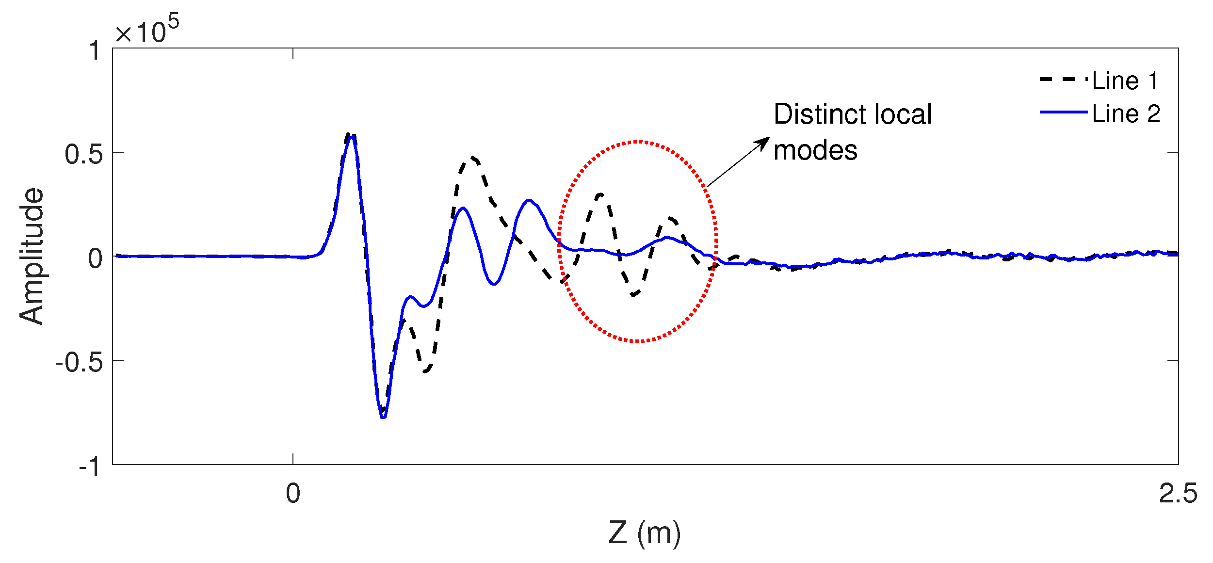
Two representative signal traces (seen in Figure 3) on Lines 1 and 2 with and without buried pipelines respectively are compared to analyze the mode difference. Distinct local modes appear around m due to the existence of pipelines. Figure 4 shows the decomposition results by EEMD on both traces. IMF1s are noise-polluted mode functions with limited physical meanings because white noises are added to signals in EEMD procedures. IMF2s, IMF5s and IMF6s present little evidence of mode difference between Lines 1 and 2, thereby not suitable for further object identification. This missing characteristic reappears in IMF3s and IMF4s, as visible oscillations exist around Z = 1 m on Line 1 (corresponding positions marked in Figure 4). Therefore, IMF3s and IMF4s on all traces of the pre-processed radargram are chosen to reconstruct the subsurface profile.
Figure 5 illustrates the reconstructed profiles by IMF3s and IMF4s respectively, which are decomposed from all signal traces. It is reasonable to eliminate the IMF signals weaker than the added white noises (amplitudes less than 500) to avoid artificial noise issues, and this would affect little on the actual modes (strength 20–40 times). In the IMF3s profile (Figure 5a), the two hyperbolic ‘tails’ of each pipeline have been eliminated. Meanwhile, the pipelines have been revealed from the noisy subterranean environment with highlighted locations and sizes. In contrast, these commendable results have not appeared as expected in the IMF4s profile (Figure 5b). Interference signals remain outside the pipeline interfaces, and near-surface signals have extended to deeper areas (from 0.75 m in Figure 2 to 1 m in Figure 5b) thereby polluting the pipeline signals. Although signals inside the pipeline portions are intensive, this reconstructed IMF4s profile is insufficient to identify the objects. Therefore, only IMF3s acquired by the developed approach can reconstruct a promising underground profile. However, unexpected visible noises appear in the deepest 10% portion, which may arise from the end effects of EEMD [29], and GPR time windows should be at least 10% larger than targeted depths in further applications.
Secondly, a numerically simulated radargram of cracked rock areas was generated by the software ‘gprMax’ [30]. ‘gprMax’ is an open source software to simulate GPR signals based on propagation physics of electromagnetic waves and the Finite-Difference Time-Domain method, widely applied in investigating signal processing approaches (e.g., [31,32]). Numerical simulation can determine the isotropy and homogeneity of the underground medium, thus ensuring object signals are not interfered by other unknown structures. Figure 6a illustrates the simulated rock profile, with the scanning length L ( m) and detection depth Z ( m). The entire section is divided into mesh grids with resolution m. Certain attributes have been assigned to the rock section, with the relative permittivity of 8, the conductivity of 0.02 S/m, the relative permeability of 1 and the magnetic loss of 0. There are three predefined cracked portions (sizes seen in the caption of Figure 6), each containing multiple randomly distributed cracks with widths of 2.5 mm, lengths and intervals ranging from 1 cm to 5 cm. These cracks are simulated as perfect electric conductors. The GPR antenna is simulated by the Ricker waveform with the central frequency of 800 MHz, while the detection time window is s. Figure 6b presents the corresponding pre-processed radargram. The pre-processing parameters are , and m. The predefined cracked areas generate not only intensive responses at their locations but also interference signals affecting other locations. Over half of the profile is occupied by GPR signals, which increases difficulties in cracked rock identification.
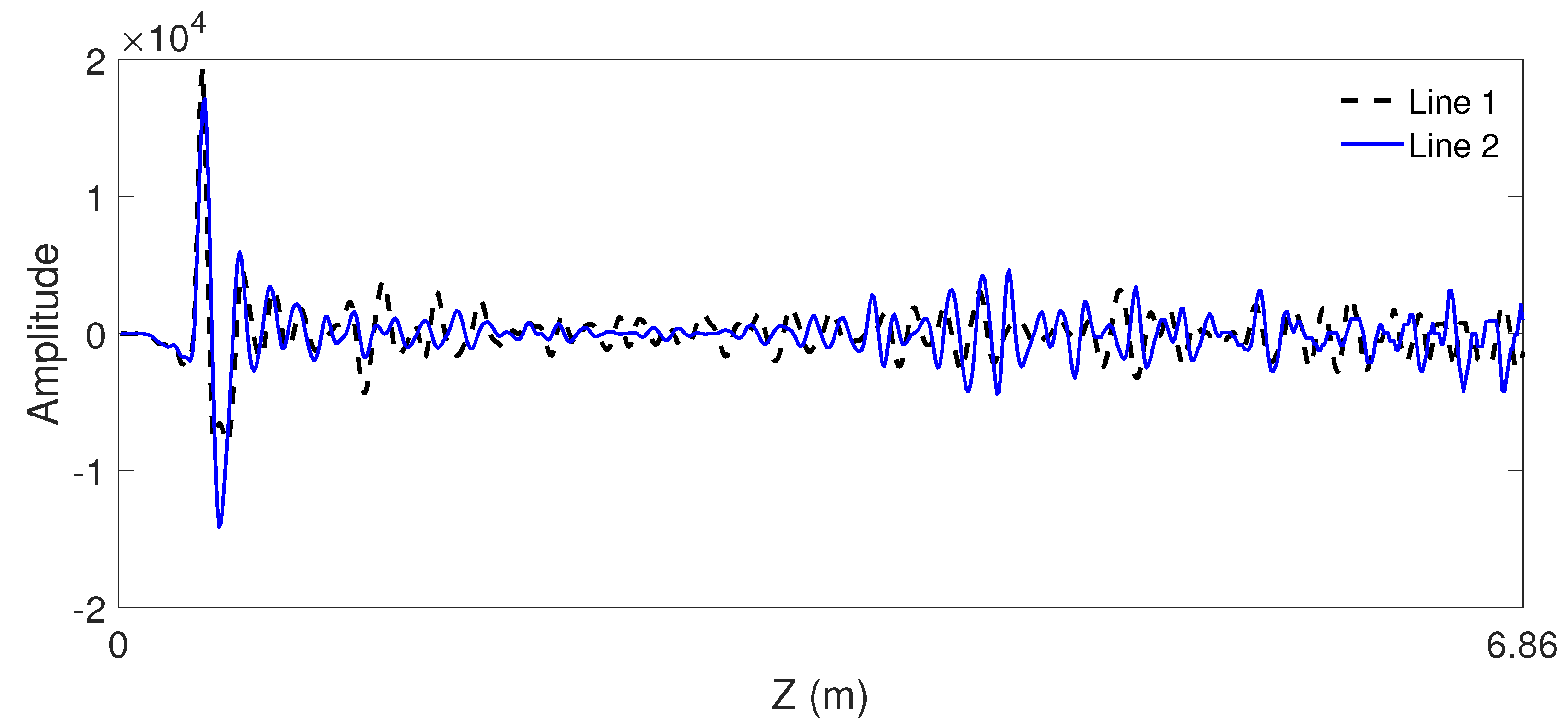
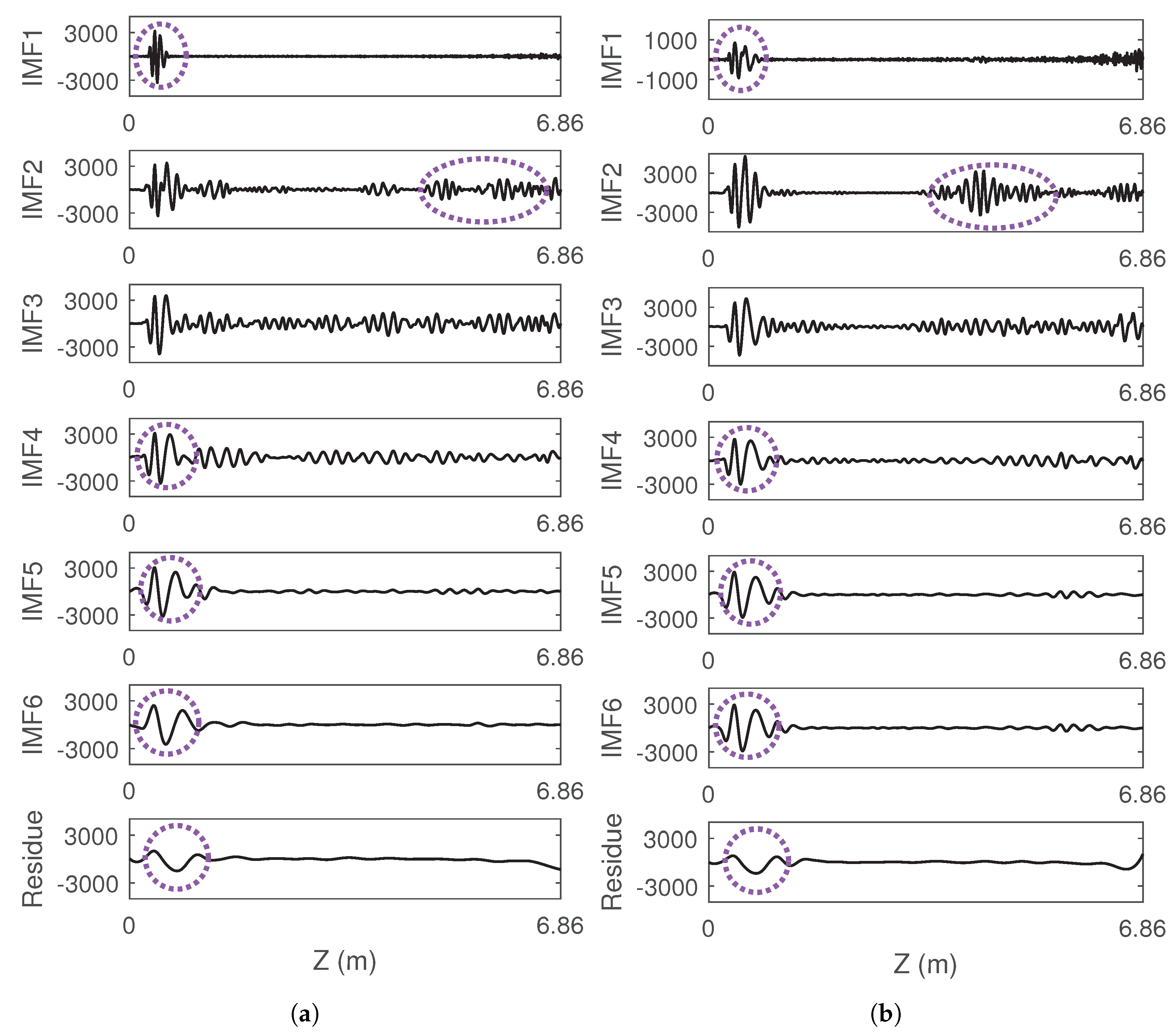
Two representative GPR traces on Lines 1 and 2 with cracks at different depths are compared to analyze the mode difference, as shown in Figure 7. The shallow cracked portion on Line 1 generates distinct local modes between 0.1 and 0.4 m depths (marked in the dotted circle). EEMD results of both traces are illustrated in Figure 8. Only mode functions after IMF5s are presented as IMF1s to IMF4s are entirely occupied by added white noises. IMF6s and IMF7s have captured the modal characteristics of both signal traces, as marked in dotted circles. However, the oscillations in IMF7s have extended beyond the actual crack depths. Therefore, IMF6s are chosen to reconstruct the GPR profile.
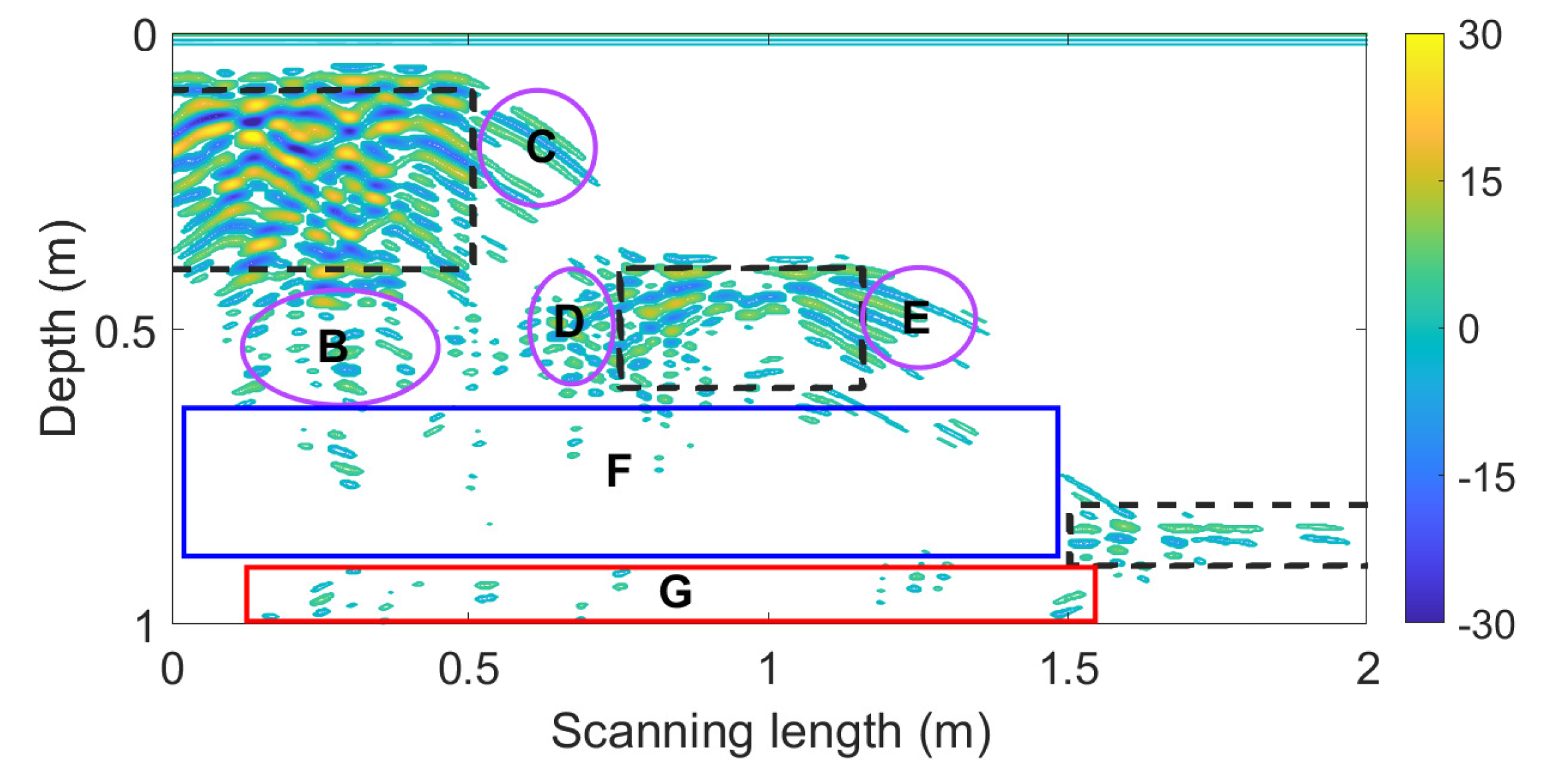
Figure 9 presents the reconstructed profile by IMF6s. Signals with amplitude weaker than 3 are eliminated since noises would affect our identification results. In the reconstructed radargram, responses are concentrated inside the cracked portions (marked as dashed rectangles), and interference signals have been almost eliminated. However, some weak signals surrounding the cracked portions are preserved (inside portions B, C, D and E) since eliminating all interference signals is difficult. Nonetheless, the intact portion F, which was covered by intensive signals in Figure 6b, has been revealed by the proposed approach. These results indicate the applicability of EEMD in distinguishing the intact and cracked rock areas. End effects sometimes occur in our decomposition procedure thus generating noises in the portion G, which indicates that GPR time windows should be at least 10% larger than targeted depths to avoid these effects.
3.2. Investigation in Field Measurement
Filed measurement was conducted in an underground cavern in Huangdao, China to evaluate the surrounding rock stability before grouting reinforcement. Figure 10 illustrates a brief scheme of detecting surrounding rock sections. A GPR instrument is attached on the cavern wall to transmit electromagnetic waves into the surrounding rocks. Once encountering the rock cracks, the electromagnetic waves will be reflected back to the receiving antenna (RA) and the response signals are recorded on the vertical trace. Owing to the wide transmission angle of the transmitting antenna (TA), reflections from non-vertical directions will generate ‘pseudo’ signals that affect the identification of those from vertical directions. Details of basic detection principles and ‘pseudo’ signals can be seen in [25]. During the investigation of the entire surrounding rock section, the GPR instrument will continuously move along the measurement direction while acquiring numerous vertical traces. In our research, a MALA 2-dimensional GPR instrument assisted by the data acquisition software ‘Groundvision’ is adopted. The central frequency of the GPR antenna is 250 MHz, and the horizontal resolution (intervals between neighbouring vertical traces) is 3 cm.
A representative subterranean section is firstly investigated to analyze the detectability of shattered rock masses by the developed approach, which is compared with the classic migration approaches (e.g., [33,34,35]) utilizing the commercial software ‘Reflexw’. The original radargram is presented in Figure 11a. Although strong reflections occur in the near-surface layers (amplitudes over 20,000), signals beneath 2 m are too weak (amplitudes below 100) for post-processing. The visible distribution in Figure 11a will differ significantly from the actual distribution due to electromagnetic attenuation, and later arrivals beneath 6 m nearly disappear in this situation. Nonetheless, the surrounding rock conditions are complicated as intensive responses have been received from most areas. Figure 11b shows the pre-processed radargram of the surrounding rock section, with the measurement length L ( m) and detection depth Z ( m). The pre-processing parameters are , and m. The depth-variant amplitude gain function has reconstructed the signals to normal levels (amplitudes around 10,000), while signals weaker than 200 (2% of normal amplitudes) have been eliminated to avoid noises. Although the right-middle area H is conveniently recognized as intact rock masses, other areas are almost covered by intensive signals, which increases difficulties in identifying the unstable structures with fragmented rocks.
Two representative measurement traces from Figure 11b, Line 1 with intermittent signals and Line 2 with later heavy signals, are decomposed to compare the local mode difference, as shown in Figure 12 and Figure 13. Besides the added white noises, IMF1s include the local mode in the near-surface layers, but this aberrant strong reflection area is not considered in the identification. Similarly, the compositions after IMF4s are also mostly occupied by the near-surface signals, unable to recognize the joint fissures at deep locations. In contrast, the IMF2 of Line 2 has captured the discernible fluctuation after 3.5 m, and this composition is chosen for further analysis.
Utilizing EEMD to decompose all vertical measurement traces, the IMF2s are preserved to reconstruct the amplitude profile of the surrounding rock section, seen in Figure 14. like the previous procedure, the IMF2 signals weaker than the added white noise (amplitudes less than 200) has been removed. For comparison, Figure 15 presents the imaging results finely processed by the commercial GPR software. The distribution of signals in areas U, W, X, Y (Figure 14) is consistent with the corresponding areas , , , (Figure 15), while signals in lower part of area V are not as intensive as the area . It is noticeable that comparing with the pre-processed profile (Figure 11), the noisy signals in area Y nearly disappear, which implies the high surrounding rock quality in this area. Although W and X are concentrated areas of fragmented rocks, the lower part of W presents higher rock quality after EEMD processing and the area X is not as cracked as shown in Figure 11. These results indicate that the developed approach has the potential to discover the subterranean joint fissures to further identify the surrounding rock stability.
3.3. Identifying Unstable Rock Structures
Two surrounding rock sections were investigated for further applying the developed approach in identifying unstable rock structures.
Figure 16 shows the original and pre-processed radargrams of a surrounding rock section, with the measurement length L ( m) and detection depth Z ( m), and the reconstructed profile by IMF2s is illustrated in Figure 17. The original radargram is insufficient for post-processing as the signals beneath 2 m are over 200 times weaker than those in the near-surface layer (amplitudes over 20,000). Later arrivals beneath 6 m are nearly invisible owing to the electromagnetic attenuation. This issue has been handled by the amplitude gain function, with pre-processed results shown in Figure 16b. However, rock identification is still difficult since intensive interference signals have nearly occupied the entire section. Contrarily, the cracked and intact rock masses are distinguishable in the reconstructed profile (Figure 17). The intact portions I, J and K that present evidence in Figure 16b have been entirely revealed, while the intact portions M and N covered by intensive signals in Figure 16b also become visible. Other areas are identified as unstable rock structures with different cracked situations, thus requiring further reinforcement measures. The deepest 10% area marked in the red rectangle is difficult to identify since the end effects of EEMD would affect this area.
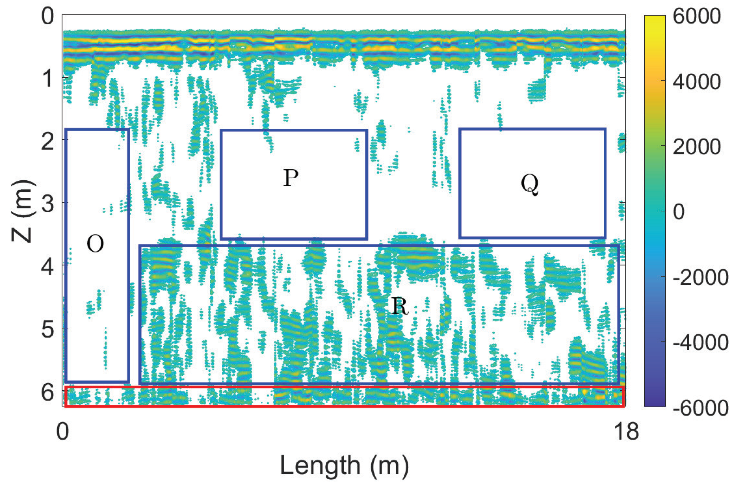
Figure 18 shows the original and pre-processed radargrams of another surrounding rock section, with the measurement length L ( m) and detection depth Z ( m), and the reconstructed profile by IMF2s is illustrated in Figure 19. Similar to the previous results, the signals beneath 2 m in the original radargram are over 200 times weaker than those from the near-surface layer (amplitudes over 20,000), which results from the electromagnetic attenuation. This issue has been handled by the amplitude gain function, with pre-processed results shown in Figure 18b. However, intensive signals have nearly occupied the entire section, making our identification difficult. Stable rock structures have been revealed after reconstructing the radargram. Different from the previous rock section in Figure 18, the deep portion R around 4–6 m of this section is almost cracked, which means the rock structure is unstable. The intact portions P and Q that show evidence in Figure 18b have been entirely revealed, while the intact portion O covered by intensive signals in Figure 18b also become visible. Therefore, our developed approach shows good practice in unstable rock structure identification. The deepest signals in the red rectangle are affected by the end effects of EEMD, and therefore the GPR time window should be 10% larger than the targeted depth in further applications.
4. Discussion and Conclusions
Two significant research developments are achieved in this paper: successfully developing mode analysis approach for complicated radargram interpretation, and successfully applying the non-destructive technology GPR for unstable rock structure identification.
Since surrounding rock quality attracted attention in underground engineering, standards to evaluate rock quality has continuously evolved, but opening and pit sampling has remained as the field detection strategy yet [36]. Although seismic velocity measurements have been utilized to indirectly estimate rock quality [37], this energy required technology is not suitable in underground caverns. GPR has been applied in object detection, stratum identification and underground water detection, but rarely in such a complicated condition with intensive wave reflection from intensive rock interfaces. Modal analysis has been applied to interpret simple GPR radargrams before, e.g., wavelet transform for de-noising [17] or pipeline identification [18] and EMD for object detection [20], but not in complicated conditions like cracked subsurface rock masses.
In this paper, an EEMD-based signal processing approach including three steps, pre-processing, signal decomposition and profile reconstruction, is investigated for interpreting GPR radargrams for unstable subsurface rock structure identification. Amplitude gain function has restored the signals to an analyzable level, against the electromagnetic attenuation which reduces the energy of responses beneath 2 m to 200 times weaker than that in the near-surface layer. The pre-processed radargrams present some different distributions with the original ones, as well as the evidence of intact rock portions (e.g., portion H in Figure 11b). By decomposing the pre-processed GPR signals into multiple IMFs and residues, one typical IMF can preserve the distinct local modes, which arise from instantaneous changes of fissure interfaces, and is chosen to reconstruct the subterranean profile. Different IMFs can present different signal features, including noises, near-surface-layer signals and object responses, while object responses can appear in different IMFs. For example, pipeline responses are preserved in the IMF3 and IMF4 in Figure 4, but only IMF3s profile can accurately show pipeline areas; simulated crack responses are preserved in the IMF6 and IMF7 in Figure 8, but oscillations in the IMF7 have extended outside the cracked portions. Choosing appropriate IMFs to reconstruct the profile is significant for further unstable rock identification.
After considering appropriate IMFs to reconstruct the radargram, the intact and cracked rock portions become distinguishable. The developed approach can eliminate the hyperbolic interference signals, but some weak signals remain surrounding the cracked portions in the numerical simulation (Figure 9). Despite these small biases, the identified cracked areas correspond well with the pre-defined ones, and the intact portion G covered by intensive signals become visible in Figure 9. In the field measurements, the intact areas that have shown evidence in pre-processed radargrams are entirely revealed (e.g., I, J and K in Figure 17, P and Q in Figure 19), while those covered by intensive signals in pre-processed radargrams also become visible (e.g., Y in Figure 14, M and N in Figure 17, O in Figure 19). Other portions containing strong responses in the reconstructed radargrams are identified as cracked areas. Our results indicate the ability of GPR assisted by the developed signal processing approach to identify shattered rock masses, which require reinforcement strategy to increase stability, and this non-destructive technology can monitoring the surrounding rock conditions during cavern operation. The end effects of EEMD would affect deepest signals, marked as red rectangles in Figure 9, Figure 17 and Figure 19, and therefore the GPR time window should be at least 10% larger than the targeted depth in further applications.
We also want to mention that this research only identifies the fissure interfaces inside the single-type rock formation (granite). Different types of rock formations can determine the rock strength that also influences the surrounding rock stability. Further research is planned in following aspects: Firstly, we will discover the quantity relationship between rock quality and GPR radargrams; secondly, we will investigate the signal processing approach to identify the rock stability with different types of rock formations; thirdly, we will investigate the quantity relationship between rock strengths with different types of rock formations and GPR signal features.
Author Contributions
Conceptualization, Y.J. and Y.D.; methodology, Y.J.; software, Y.J.; validation, Y.J. and Y.D.; formal analysis, Y.J. and Y.D.; investigation, Y.J. and Y.D.; writing—original draft preparation, Y.J.; writing—review and editing, Y.D. and Y.J.; visualization, Y.J.; supervision, Y.D. All authors have read and agreed to the published version of the manuscript.
Funding
This research received no external funding.
Acknowledgments
Xuefei Wei, Pinning Huang, and Jinming Feng in Hydraulic Engineering, Tsinghua University have kindly provided help in this research. The authors thank Wei for cooperation in data acquisition as well as agreement to publish the data. Feng’s work on managing the instruments and experiments is appreciated. The authors thank Huang for programming support.
Conflicts of Interest
The authors declare no conflict of interest.
Abbreviations
The following abbreviations are used in this manuscript:
| GPR | Ground penetrating radar |
| EMD | Empirical mode decomposition |
| EEMD | Ensemble empirical mode decomposition |
| IMF | Intrinsic mode function |
References
- Matos, C.R.; Carneiro, J.F.; Silva, P.P. Overview of large-scale underground energy storage technologies for integration of renewable energies and criteria for reservoir identification. J. Energy Storage 2019, 21, 241–258. [Google Scholar] [CrossRef]
- Costa, A.L.; Sousa, R.L.; Einstein, H.H. Probabilistic 3D alignment optimization of underground transport infrastructure integrating GIS-based subsurface characterization. Tunn. Undergr. Space Technol. 2018, 72, 233–241. [Google Scholar] [CrossRef]
- Kang, H.P.; Zhang, X.; Si, L.P.; Wu, Y.; Gao, F. In-situ stress measurements and stress distribution characteristics in underground coal mines in China. Eng. Geol. 2010, 116, 333–345. [Google Scholar] [CrossRef]
- Hoek, E.; Marinos, P.; Benissi, M. Applicability of the Geological Strength Index (GSI) classification for very weak and sheared rock masses. The case of the Athens Schist Formation. Bull. Eng. Geol. Environ. 1998, 57, 151–160. [Google Scholar] [CrossRef]
- Kong, P.; Jiang, L.; Shu, J.; Sainoki, A.; Wang, Q. Effect of fracture heterogeneity on rock mass stability in a highly heterogeneous underground roadway. Rock Mech. Rock Eng. 2019, 52, 4547–4564. [Google Scholar] [CrossRef]
- Li, S.; Vaziri, V.; Kapitaniak, M.; Millett, J.M.; Wiercigroch, M. Application of Resonance Enhanced Drilling to coring. J. Pet. Sci. Eng. 2020, 188, 106866. [Google Scholar] [CrossRef]
- Liang, M.; Fang, X. Application of fiber Bragg grating sensing technology for bolt force status monitoring in roadways. Appl. Sci. 2018, 8, 107. [Google Scholar] [CrossRef] [Green Version]
- Lei, X.; Xue, Z.; Hashimoto, T. Fiber optic sensing for geomechanical monitoring:(2)-distributed strain measurements at a pumping test and geomechanical modeling of deformation of reservoir rocks. Appl. Sci. 2019, 9, 417. [Google Scholar] [CrossRef] [Green Version]
- Davis, J.L.; Annan, A.P. Ground-penetrating radar for high-resolution mapping of soil and rock stratigraphy 1. Geophys. Prospect. 1989, 37, 531–551. [Google Scholar] [CrossRef]
- Agapiou, A.; Sarris, A. Working with Gaussian Random Noise for Multi-Sensor Archaeological Prospection: Fusion of Ground Penetrating Radar Depth Slices and Ground Spectral Signatures from 0.00 m to 0.60 m below Ground Surface. Remote Sens. 2019, 11, 1895. [Google Scholar] [CrossRef] [Green Version]
- Dong, Z.; Ye, S.; Gao, Y.; Fang, G.; Zhang, X.; Xue, Z.; Zhang, T. Rapid detection methods for asphalt pavement thicknesses and defects by a vehicle-mounted ground penetrating radar (GPR) system. Sensors 2016, 16, 2067. [Google Scholar] [CrossRef] [PubMed] [Green Version]
- Liu, H.; Long, Z.; Han, F.; Fang, G.; Liu, Q.H. Frequency-Domain Reverse-Time Migration of Ground Penetrating Radar Based on Layered Medium Green’s Functions. IEEE J. Sel. Top. Appl. Earth Obs. Remote Sens. 2018, 11, 2957–2965. [Google Scholar] [CrossRef]
- Jazayeri, S.; Klotzsche, A.; Kruse, S. Improving estimates of buried pipe diameter and infilling material from ground-penetrating radar profiles with full-waveform inversion. Geophysics 2018, 83, H27–H41. [Google Scholar] [CrossRef]
- Tong, Z.; Gao, J.; Yuan, D. Advances of deep learning applications in ground-penetrating radar: A survey. Constr. Build. Mater. 2020, 258, 120371. [Google Scholar] [CrossRef]
- Kang, M.S.; Kim, N.; Lee, J.J.; An, Y.K. Deep learning-based automated underground cavity detection using three-dimensional ground penetrating radar. Struct. Health Monit. 2020, 19, 173–185. [Google Scholar] [CrossRef]
- Jin, Y.; Duan, Y. A new method for abnormal underground rocks identification using ground penetrating radar. Measurement 2020, 149, 106988. [Google Scholar] [CrossRef]
- Baili, J.; Lahouar, S.; Hergli, M.; Al-Qadi, I.L.; Besbes, K. GPR signal de-noising by discrete wavelet transform. NDT E Int. 2009, 42, 696–703. [Google Scholar] [CrossRef]
- Ni, S.H.; Huang, Y.H.; Lo, K.F.; Lin, D.C. Buried pipe detection by ground penetrating radar using the discrete wavelet transform. Comput. Geotech. 2010, 37, 440–448. [Google Scholar] [CrossRef]
- Addison, A.D.; Battista, B.M.; Knapp, C.C. Improved hydrogeophysical parameter estimation from empirical mode decomposition processed ground penetrating radar data. J. Environ. Eng. Geophys. 2009, 14, 171–178. [Google Scholar] [CrossRef] [Green Version]
- Wu, X.; Senalik, C.A.; Wacker, J.; Wang, X.; Li, G. Object detection of ground-penetrating radar signals using empirical mode decomposition and dynamic time warping. Forests 2020, 11, 230. [Google Scholar] [CrossRef] [Green Version]
- Huang, N.E.; Shen, Z.; Long, S.R.; Wu, M.C.; Shih, H.H.; Zheng, Q.; Yen, N.; Tung, C.C.; Liu, H.H. The empirical mode decomposition and the Hilbert spectrum for nonlinear and non-stationary time series analysis. Proc. Math. Phys. Eng. Sci. 1998, 454, 903–995. [Google Scholar] [CrossRef]
- Fang, L.; Sun, H. Study on EEMD-Based KICA and Its Application in Fault-Feature Extraction of Rotating Machinery. Appl. Sci. 2018, 8, 1441. [Google Scholar] [CrossRef] [Green Version]
- Roshanmanesh, S.; Hayati, F.; Papaelias, M. Utilisation of Ensemble Empirical Mode Decomposition in Conjunction with Cyclostationary Technique for Wind Turbine Gearbox Fault Detection. Appl. Sci. 2020, 10, 3334. [Google Scholar] [CrossRef]
- Wu, Z.; Huang, N.E. Ensemble empirical mode decomposition: A noise-assisted data analysis method. Adv. Adapt. Data Anal. 2009, 1, 1–41. [Google Scholar] [CrossRef]
- Cassidy, N.J. Ground Penetrating Radar Data Processing, Modelling and Analysis. In Ground Penetrating Radar Theory and Applications; Jol, H.M., Ed.; Elsevier: Amsterdam, The Netherlands, 2008. [Google Scholar]
- Benedetto, A.; Tosti, F.; Ciampoli, L.B.; D’amico, F. An overview of ground-penetrating radar signal processing techniques for road inspections. Signal Process. 2017, 132, 201–209. [Google Scholar] [CrossRef]
- Zheng, J.; Cheng, J.; Yang, Y. Partly ensemble empirical mode decomposition: An improved noise-assisted method for eliminating mode mixing. Signal Process. 2014, 96, 362–374. [Google Scholar] [CrossRef]
- Chen, X.; Cui, B. Efficient modeling of fiber optic gyroscope drift using improved EEMD and extreme learning machine. Signal Process. 2016, 128, 1–7. [Google Scholar] [CrossRef]
- He, Z.; Shen, Y.; Wang, Q.; Wang, Y.; Feng, N.; Ma, L. Mitigating end effects of EMD using non-equidistance grey model. J. Syst. Eng. Electron. 2012, 23, 603–611. [Google Scholar] [CrossRef]
- Warren, C.; Giannopoulos, A.; Giannakis, I. gprMax: Open source software to simulate electromagnetic wave propagation for Ground Penetrating Radar. Comput. Phys. Commun. 2016, 209, 163–170. [Google Scholar] [CrossRef] [Green Version]
- Alsharahi, G.; Faize, A.; Louzazni, M.; Mostapha, A.M.M.; Bayjja, M.; Driouach, A. Detection of cavities and fragile areas by numerical methods and GPR application. J. Appl. Geophys. 2019, 164, 225–236. [Google Scholar] [CrossRef]
- Meşecan, İ.; Çiço, B.; Bucak, İ.Ö. Feature vector for underground object detection using B-scan images from GprMax. Microprocess. Microsyst. 2020, 76, 103116. [Google Scholar] [CrossRef]
- Moran, M.L.; Greenfield, R.J.; Arcone, S.A.; Delaney, A.J. Multidimensional GPR array processing using Kirchhoff migration. J. Appl. Geophys. 2000, 43, 281–295. [Google Scholar] [CrossRef]
- Leuschen, C.J.; Plumb, R.G. A matched-filter-based reverse-time migration algorithm for ground-penetrating radar data. IEEE Trans. Geosci. Remote Sens. 2001, 39, 929–936. [Google Scholar] [CrossRef] [Green Version]
- Smitha, N.; Bharadwaj, D.U.; Abilash, S.; Sridhara, S.N.; Singh, V. Kirchhoff and FK migration to focus ground penetrating radar images. Int. J. Geo-Eng. 2016, 7, 4. [Google Scholar] [CrossRef] [Green Version]
- Zhang, L. Determination and applications of rock quality designation (RQD). J. Rock Mech. Geotech. Eng. 2016, 8, 389–397. [Google Scholar] [CrossRef] [Green Version]
- Andy, A.B.; Rosli, S. Correlation of seismic P-wave velocities with engineering parameters (N value and rock quality) for tropical environmental study. Int. J. Geosci. 2012, 3, 749–757. [Google Scholar]
Figure 1.
(a) Representative ground penetrating radar (GPR) signals from two measurement traces with and without buried objects beneath respectively. (b) Fast Fourier transform results of these two signal series.
Figure 1.
(a) Representative ground penetrating radar (GPR) signals from two measurement traces with and without buried objects beneath respectively. (b) Fast Fourier transform results of these two signal series.

Figure 2.
GPR signal amplitude profile of two pre-buried pipelines after pre-processing.

Figure 3.
GPR signals of Line 1 and 2 from pipeline detection with initialized duration.

Figure 4.
(a) Intrinsic mode functions (IMFs) and residue of Line 1 signals from pipeline detection decomposed by EEMD. (b) IMFs and residue of Line 2 signals from pipeline detection decomposed by EEMD.
Figure 4.
(a) Intrinsic mode functions (IMFs) and residue of Line 1 signals from pipeline detection decomposed by EEMD. (b) IMFs and residue of Line 2 signals from pipeline detection decomposed by EEMD.

Figure 5.
(a) IMF3s amplitude profile of 2 pre-buried pipelines. (b) IMF4s amplitude profile of 2 pre-buried pipelines. Signals with amplitudes less than 500 are removed.
Figure 5.
(a) IMF3s amplitude profile of 2 pre-buried pipelines. (b) IMF4s amplitude profile of 2 pre-buried pipelines. Signals with amplitudes less than 500 are removed.

Figure 6.
(a) Simulated rock sections with three cracked areas ( m and m, m and m, m and m). (b) The corresponding radargram after pre-processing.
Figure 6.
(a) Simulated rock sections with three cracked areas ( m and m, m and m, m and m). (b) The corresponding radargram after pre-processing.

Figure 7.
GPR signals of Line 1 and 2 from numerical simulation with initialized duration.

Figure 8.
(a) IMFs and residue of Line 1 signals from pipeline detection decomposed by EEMD. (b) IMFs and residue of Line 2 signals from pipeline detection decomposed by EEMD.
Figure 8.
(a) IMFs and residue of Line 1 signals from pipeline detection decomposed by EEMD. (b) IMFs and residue of Line 2 signals from pipeline detection decomposed by EEMD.

Figure 9.
IMF6s amplitude profile of the simulated cracked surrounding rock section.

Figure 10.
A brief scheme of detecting surrounding rock sections by GPR.

Figure 11.
(a) IMFs and residue of Line 1 signals from the cavern detection decomposed by EEMD. (b) IMFs and residue of Line 2 signals from the cavern detection decomposed by EEMD.
Figure 11.
(a) IMFs and residue of Line 1 signals from the cavern detection decomposed by EEMD. (b) IMFs and residue of Line 2 signals from the cavern detection decomposed by EEMD.

Figure 12.
Pre-processed GPR signals of Lines 1 and 2 from the cavern detection.

Figure 13.
(a) IMFs and residue of Line 1 signals from the cavern detection decomposed by EEMD. (b) IMFs and residue of Line 2 signals from the cavern detection decomposed by EEMD. All the mode features are marked in dotted circles.
Figure 13.
(a) IMFs and residue of Line 1 signals from the cavern detection decomposed by EEMD. (b) IMFs and residue of Line 2 signals from the cavern detection decomposed by EEMD. All the mode features are marked in dotted circles.

Figure 14.
IMF2s amplitude profile of the cavern detection. Signals with amplitudes less than 200 are removed.
Figure 14.
IMF2s amplitude profile of the cavern detection. Signals with amplitudes less than 200 are removed.

Figure 15.
Imaging results of finely processed GPR data by GPR commercial software.

Figure 16.
(a) Original GPR radargram of a surrounding rock section. (b) Corresponding pre-processed radargram (signals with amplitudes less than 500 are removed).
Figure 16.
(a) Original GPR radargram of a surrounding rock section. (b) Corresponding pre-processed radargram (signals with amplitudes less than 500 are removed).

Figure 17.
IMF2s amplitude profile of the surrounding rock section in Figure 16. Signals with amplitudes less than 500 are removed.
Figure 17.
IMF2s amplitude profile of the surrounding rock section in Figure 16. Signals with amplitudes less than 500 are removed.

Figure 18.
(a) Original GPR radargram of another surrounding rock section. (b) Corresponding pre-processed radargram (signals with amplitudes less than 500 are removed).
Figure 18.
(a) Original GPR radargram of another surrounding rock section. (b) Corresponding pre-processed radargram (signals with amplitudes less than 500 are removed).

Figure 19.
IMF2s amplitude profile of the surrounding rock section in Figure 18. Signals with amplitudes less than 500 are removed.
Figure 19.
IMF2s amplitude profile of the surrounding rock section in Figure 18. Signals with amplitudes less than 500 are removed.

Publisher’s Note: MDPI stays neutral with regard to jurisdictional claims in published maps and institutional affiliations. |
© 2020 by the authors. Licensee MDPI, Basel, Switzerland. This article is an open access article distributed under the terms and conditions of the Creative Commons Attribution (CC BY) license (http://creativecommons.org/licenses/by/4.0/).
Share and Cite
MDPI and ACS Style
Jin, Y.; Duan, Y. Identification of Unstable Subsurface Rock Structure Using Ground Penetrating Radar: An EEMD-Based Processing Method. Appl. Sci. 2020, 10, 8499. https://doi.org/10.3390/app10238499
AMA Style
Jin Y, Duan Y. Identification of Unstable Subsurface Rock Structure Using Ground Penetrating Radar: An EEMD-Based Processing Method. Applied Sciences. 2020; 10(23):8499. https://doi.org/10.3390/app10238499
Chicago/Turabian StyleJin, Yang, and Yunling Duan. 2020. "Identification of Unstable Subsurface Rock Structure Using Ground Penetrating Radar: An EEMD-Based Processing Method" Applied Sciences 10, no. 23: 8499. https://doi.org/10.3390/app10238499
Note that from the first issue of 2016, this journal uses article numbers instead of page numbers. See further details here.