Depth Dependence and Keyhole Stability at Threshold, for Different Laser Welding Regimes

Featured Application

Scaling laws of keyhole depths are derived for different laser welding regimes. Recommended operating conditions are proposed in order to reduce the risk of weld seam defects.

Abstract

Depending of the laser operating parameters, several characteristic regimes of laser welding can be observed. At low welding speeds, the aspect ratio of the keyhole can be rather large with a rather vertical cylindrical shape, whereas at high welding speeds, low aspect ratios result, where only the keyhole front is mainly irradiated. For these different regimes, the dependence of the keyhole (KH) depth or the keyhole threshold, as a function of the operating parameters and material properties, is derived and their resulting scaling laws are surprisingly very similar. This approach allows us to analyze the keyhole behavior for these welding regimes, around their keyhole generation thresholds. Specific experiments confirm the occurrence and the behavior of these unstable keyholes for these conditions. Furthermore, recent experimental results can be analyzed using these approaches. Finally, this analysis allows us to define the aspect ratio range for the occurrence of this unstable behavior and to highlight the importance of laser absorptivity for this mechanism. Consequently, the use of a short wavelength laser for the reduction of these keyhole stability issues and the corresponding improvement of weld seam quality is emphasized.

1. Introduction

Laser welding has become an extremely widely used process in the industrial world because it allows the easy assembly of metal parts having a great range of thicknesses and with a very high productivity. All these processes operate in the so-called keyhole (KH) mode; i.e., the laser radiation penetrates the material to a depth at least greater than the focal spot. Thanks to this effect, in a regime that can be described as conventional “macro-welding,” it is possible to assemble thicknesses of about ten millimeters, at welding speeds of a few m/min, using lasers delivering powers of a few tens of kW and focal spots of several hundred microns. At the other end of the range of operating parameters, there is a more dynamic regime, the so-called “micro-welding” regime, which uses lasers of a few hundred watts and focal spots typically smaller than a hundred microns. Sub-millimeter thicknesses can then be welded, but at very high welding speeds, typically of several m/s. One must also note that these conditions are met for example, in additive powder bed manufacturing processes [1,2].

A crucial point in the implementation of this process is the knowledge of the depths of the KH obtained, as a function of these operating and thermo-physical parameters of the material used. In order to estimate these depths, many semi-analytical [3,4,5,6,7,8] or numerical [9,10,11,12,13,14,15] approaches have been considered. We had also recently proposed a relatively efficient and simple model [16] for estimating these KH depths based on a purely thermal analysis of the mechanisms involved, which makes it possible to reproduce quite satisfactorily the experimental results of this “macro-welding” regime, obtained with various operating parameters and on materials with very different thermo-physical properties.

However, it turned out that this model could also reproduce the experimental results obtained in the “micro-welding” regime, in particular, those obtained in the context of additive manufacturing experiments [17,18,19], which seemed rather surprising, given that in this regime the geometries of the KHs present are very different from those observed in a “macro-welding” regime. Indeed, Berger and Hügel [20] have shown that at high welding speeds, which could also characterize this “micro-welding” regime, the interaction of the incident laser must mainly take place on the inclined front wall of the KH and not inside the quasi-vertical cylindrical KH characteristic of the macro-welding regime. Experimental visualizations of the KH shapes by time-resolved X-ray radiography have directly confirmed this geometry [21,22].

For this reason, in order to explain these results, an original model adapted to this inclined KH front is proposed here. It is based on a generalization of the well-known “piston model” developed by Semak—Matsunawa [23] and allows for reproducing and interpreting the experimental results of Cunnigham et al. [21]. It also makes it possible to estimate all the relevant parameters of this interaction regime—the incident power dependence on the resulting aspect ratio, the inclination of the KH front and the velocity of rearward liquid ejection—and to quantify the threshold power, allowing for the appearance of KH; i.e., when the aspect ratio becomes greater or equal to one. As a consequence, the analysis of these KH depths scaling laws also shows that for these threshold conditions, an unstable behavior of the melt pool which has never been shown before should appear. The influences of the main parameters controlling this unstable behavior, particularly the laser absorptivity of the material, are also analyzed.

This paper is organized as follows: the model describing the thermal approach used for the analysis of KH depths in the macro-welding regime is briefly recalled in Section 2. It allows comparing its resulting scaling laws with those obtained in the dynamic regime, as described in Section 3, where the incident laser beam mainly impinges the inclined KH front. Section 3 also contains the geometrical aspects of the KH front, the resulting scaling laws and a comparison with related experiments. In Section 4, as a consequence of the similarity of resulting scaling laws, the stability issues near the KH threshold are discussed, and corresponding experiments can be explained by the proposed mechanism. Appendix A contains the detailed equations used for the description of this generalized piston model (GPM).

2. Thermal Model for High Aspect Ratio Keyholes

2.1. Model for Deep Penetration Regime

We recall here the model that allows determining the dependence of the KH depth in the case of keyholes with rather large aspect ratios R = e/d where e is defined as the KH depth and d is the spot diameter [16]. For this regime, one considers that the KH is a vertical cylinder with a diameter d given by the spot diameter, whose wall is at a uniform evaporation temperature T_v, which is moving with a welding speed V_w inside a material at initial temperature T₀. The incident laser power P is homogeneously distributed inside the KH due to the multiple reflection process. Only the heat conduction loss process from the KH wall is taken into account. As the aspect ratio R is large for this deep penetration regime, the heat flux from the KH wall is considered mainly 2D, so the power loss per unit keyhole depth dP/dz (W/m) for this geometry can be rather easily determined for this cylindrical geometry [16,24,25] and is given by:

$$\frac{\mathrm{dP}}{\mathrm{dz}}=\mathrm{K}\left({\mathrm{T}}_{\mathrm{v}}{-\mathrm{T}}_0\right)\mathrm{g}\left(\mathrm{Pe}\right)$$

(1)

where K is heat conductivity of the solid material and g(Pe) is a function of the Peclet number Pe (Pe = V_wd/(2κ) where κ is the solid heat diffusivity). The function g(Pe) has to be computed numerically, but for a given range of Peclet numbers, one can use a simple and useful linear approximation g(Pe) ≈ mPe + n. For example, many laser welding processes are characterized by a Peclet range 2 ≤ Pe ≤ 10; in that range, one determines that m ≈ 2.4 and n ≈ 3 [16].

As the absorbed laser power A(R)P is homogeneously distributed along the KH depth e, it is then given by (P—incident power, and A(R)—KH absorptivity which depends of its aspect ratio R = e/d):

$$\mathrm{e}=\frac{\mathrm{A}\left(\mathrm{R}\right)\mathrm{P}}{\raisebox{1ex}{$\mathrm{dP}$}\!\left/ \!\raisebox{-1ex}{$\mathrm{dz}$}\right.}=\frac{\mathrm{A}\left(\mathrm{R}\right)\mathrm{P}}{\mathrm{K}\left({\mathrm{T}}_{\mathrm{v}}-{\mathrm{T}}_0\right)\left(\mathrm{mPe}+\mathrm{n}\right)},$$

(2)

From Equation (2), the aspect ratio R = e/d is then written as:

$$\mathrm{R}=\frac{{\mathrm{R}}_0}{\left(1+\frac{{\mathrm{V}}_{\mathrm{w}}}{{\mathrm{V}}_0}\right)},$$

(3)

where R₀ = A(R)P/(ndK(T_v − T₀) and V₀ = 2nκ /(md) have been defined.

Equation (3) reproduces the KH depth variation that is usually observed for the macro-welding experiments, and its dependence with the characteristic thermo-physical properties of the material: at high welding speeds V_w, the KH depth is inversely proportional to the welding speed, whereas when the welding speed decreases, R increases and then saturates. Another way to write Equation (3) is the following:

$$\frac{\mathrm{A}\left(\mathrm{R}\right)\mathrm{P}}{\left(\mathrm{dR}\right)}=\mathrm{a}+\mathrm{b}\left({\mathrm{V}}_{\mathrm{w}}\mathrm{d}\right),$$

(4)

where

a = nK(T_v − T₀) and b = mK(T_v − T₀)/(2κ),

(5)

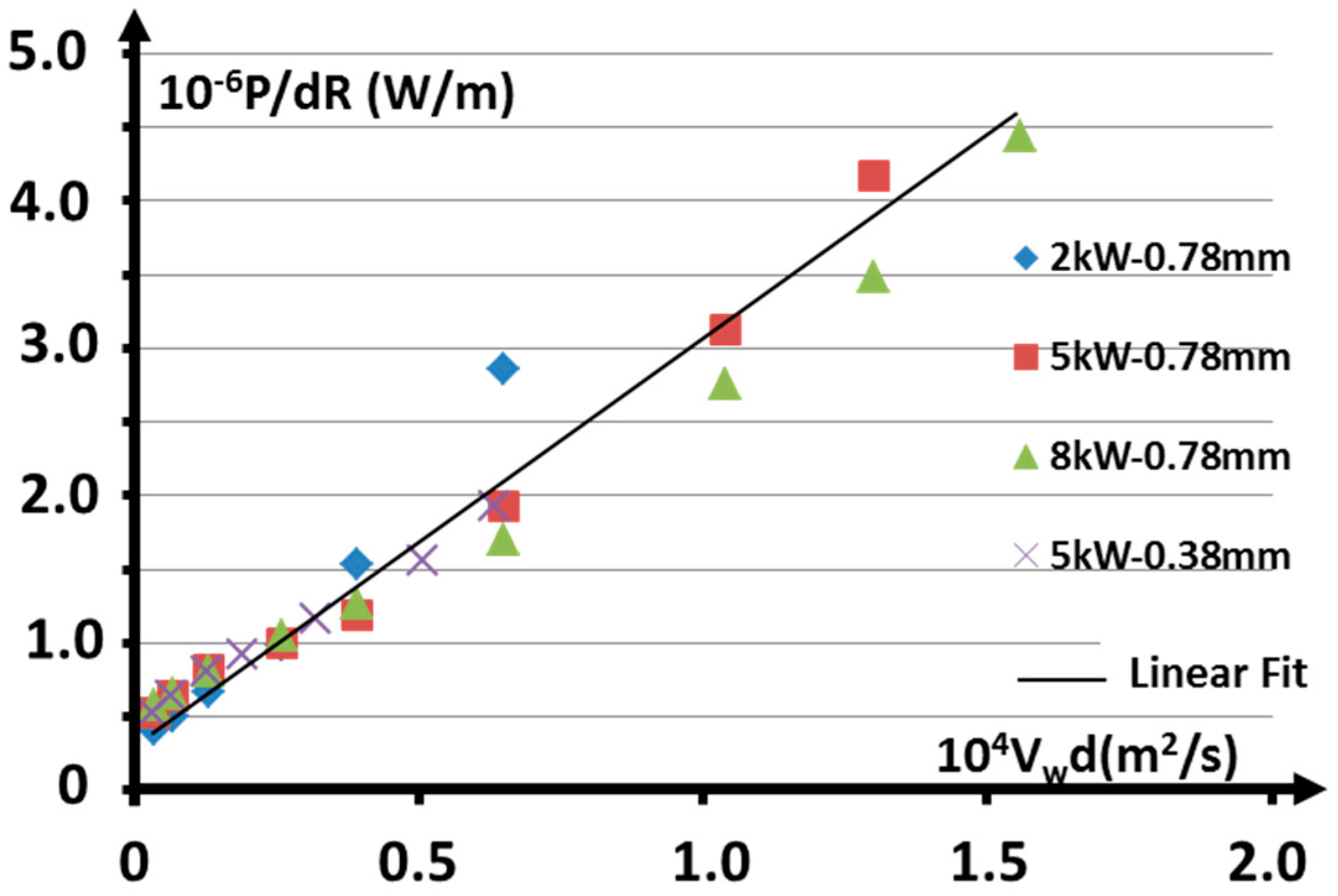
Equation (4) is interesting because its shows that the variable A(R)P/(dR) is a linear function of the variable V_wd—both depend only on the operating parameters—and the slope b and the ordinate at the origin a of this linear function depend only on the thermo-physical properties of the material and the conductive loss (through the dependence in m and n, which is defined by the shape of the KH used).

The scaling law described by Equation (4) has been verified for different published data obtained for several macro-experiments with different materials, such as steel [26] and copper [27]. Figure 1 shows an example of this comparison for experiments realized on St35 steel and different laser powers and focal spot diameters [26]. The observed correct agreement between this rather simple model and the corresponding macro-experiments shows that this model contains the main parameters involved for the determination of the scaling law for the KH depth.

Additionally, from Equation (4) it is possible to consider an important parameter, which is the incident power threshold P_t necessary for obtaining an aspect ratio R = 1. From Equation (4), P_t is then defined by:

$$\frac{{\mathrm{P}}_{\mathrm{t}}}{\mathrm{d}}=\frac{(\mathrm{a}+\mathrm{b}\left({\mathrm{V}}_{\mathrm{w}}\mathrm{d}\right)}{\mathrm{A}\left(1\right)}$$

(6)

where A(1) would be some characteristic absorptivity of the KH when its aspect ratio R = 1. One will see in the next section that the scaling of P_t given by Equation (6) is a decisive parameter controlling the geometry of the KH front. Finally, taking into account Equations (4) and (6), one must notice that R can be written in a more general form:

$$\mathrm{R}=\frac{\mathrm{A}\left(\mathrm{R}\right)}{\mathrm{A}\left(1\right)}\frac{\mathrm{P}}{{\mathrm{P}}_{\mathrm{t}}}$$

(7)

which will be also observed for the dynamic model in Section 3.

3. Dynamic Model for Low Aspect Ratio Keyholes or High Welding Speeds

3.1. Geometry of the KH Front at High Welding Speed

For a given material, an incident laser power and focusing conditions, when the welding speed is increased, Equation (3) shows that the KH depth decreases. But this scheme of a vertical cylindrical KH is no longer valid at high welding speeds: experimentally, one observes that the KH front is inclined and this inclination increases with the welding speed, so the vertical incident laser beam impinges this part (Figure 2b). Therefore, the model described in Section 2 should no longer be used for determining the KH depth for these regimes.

In fact, this KH depth mainly results from the KH front inclination that is a function of the operating parameters. The reflected beam on this inclined KH front has a mean inclination that is twice the inclination angle α of the KH front. At high welding speeds, the contribution of this reflected beam to the final KH depth is small compared to the first contribution of the vertical incident beam, because of its large inclination 2α and its decreased intensity resulting from its first reflection [28,29]. This point is confirmed by the X-ray radiographies of the KH by Cunnigham et al. [21] and Kouraytem et al. [22] where one can see that the KH depth is mainly defined by the impact of the direct beam for a range of aspect ratio of R < ≈3. Accordingly, in order to estimate the KH depth for these conditions, only the contribution of the first impact of the vertical incident beam on the KH front is considered in the model that will be discussed in the next Section 3.2.

With this geometry where α is the inclination angle of the KH front, it is easy to define that the characteristic aspect ratio R is given by:

$$\mathrm{R}=\frac{\mathrm{e}}{\mathrm{d}}=\frac{1}{\mathrm{tg}(\mathsf{\alpha })},$$

(8)

and therefore, this analysis will be restricted to rather low aspect ratios R < ≈3.

3.2. Generalized Piston Model for High Welding Speeds

A possible way to solve this problem is to first consider that the KH front is stationary in the frame of the laser beam. In fact, in this laser beam frame, the displacement of this KH front results of the vectorial addition of the horizontal welding speed V_w and a “drilling” speed V_d that is directed along the normal to the local surface. This drilling velocity V_d results from the recoil pressure due to the local evaporation process that pushes this surface inside the material by expelling the liquid metal along the sides of this surface, which is then ejected rearwards toward the melt pool. This process is similar to the well-known “piston model” initially described by Semak and Matsunawa [23] for the drilling process, but applied here on an inclined surface. Now, as this KH front is stationary in the laser beam frame, this means that the resulting normal speed of this surface is zero. As a result, the stationarity of the KH front in the laser beam frame is fulfilled when [29]:

V_d = V_w cos(α),

(9)

Therefore, in order to compute the inclination angle α, it is this Equation (9) that must be added to the set of equations describing the process of “drilling,” determining the drilling velocity V_d. The equations used for the physical model describing the “piston model” allowing the determination of V_d are described in detail in Appendix A.

The piston model initially used for describing the drilling process involved a circular disk whose diameter is equal to the spot diameter that is moving at a speed V_d inside the material [23]. But in the present case of dynamic welding, high speed video visualizations of the KH front show that its surface is rather close to a half-cone shape, which is inclined by the high welding speed. This half-cone shape of the KH can be understood because we are dealing with KHs with rather low aspect ratios, unlike the usual high aspect ratios KHs characteristic of macro-welding regimes that would rather have a cylindrical shape.

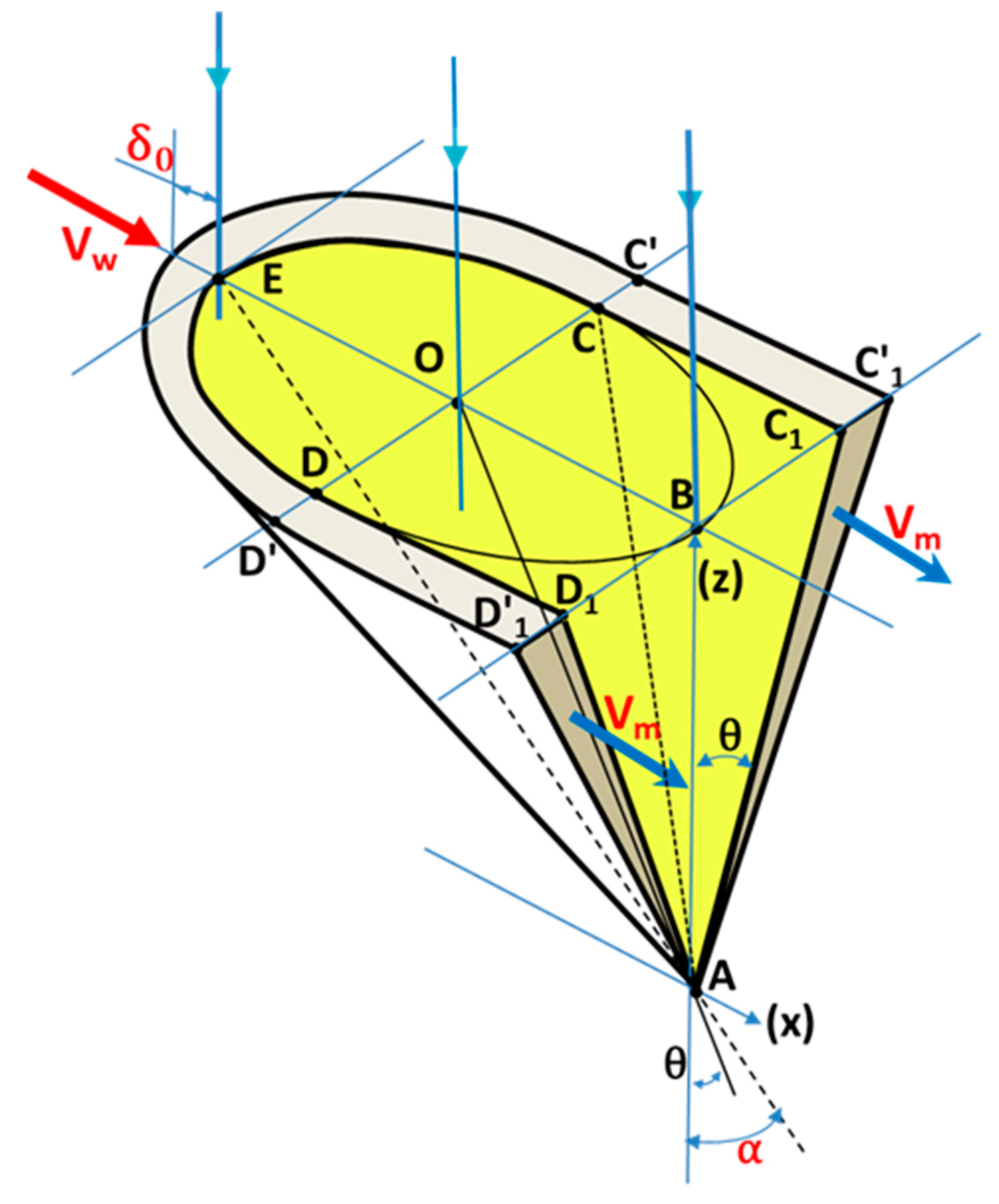
The scheme of the KH front that has been used for the characterizations of the resulting aspect ratios for these conditions is therefore shown in Figure 3. It shows all the geometrical parameters used for the application of this generalized piston model. The KH front inclination α is defined in the symmetry plane of the half-cone shape. We have also considered that the thickness of the melt layer flowing around this shape decreases linearly along its depth, and this liquid is ejected rearwards with a mean velocity V_m by this process. The three equations for mass, momentum and energy conservation, and those describing the recoil pressure, the melt thickness and the Fresnel surface absorptivity, are detailed in Appendix A; only the main results of this model are discussed in the following Section 3.3.

3.3. Results of the Generalized Piston Model for High Welding Speeds

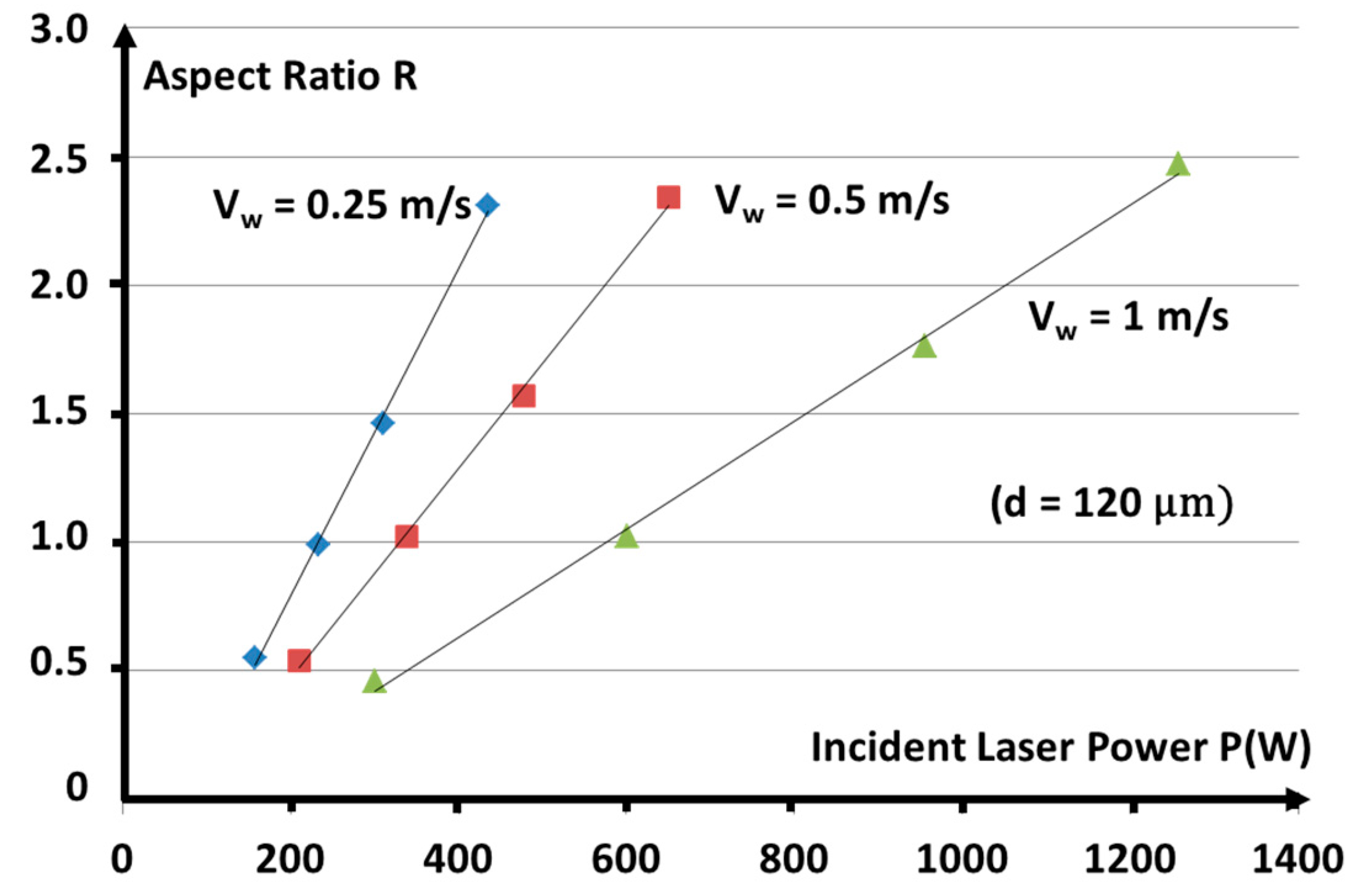
An example of the application of this model is discussed now, using experimental conditions close to the experiments on Ti-6Al-4V material, published by Cunningham et al. [21] where the results of experiments realized with a rather large set of operating parameters (incident laser power and welding speed) are available for discussion. In our model, we used three spot diameters (60, 120 and 180 μm), with three welding speeds V_w (0.25, 0.5 and 1 m/s) and four different incident laser powers, in order to scan aspect ratios from 0.5 to 3.

An example of the resulting aspect ratios R, defined by Equation (8), has been plotted on Figure 4 as a function of the incident power P, for three different welding speeds V_w. For a given welding speed V_w, one can first observe that the aspect ratio R is a linear function of the incident power, which can be written as:

R ≈ r₀ (P(W) − P′),

(10)

where the slope r₀ of this linear function and P’, the extrapolated threshold of laser power for the beginning of penetration, are dependent of the welding speed V_w, and of the spot diameter d. It is also interesting to notice that the inverse of the slope r₀ appears to be a linear function of the welding speed, 1/r₀ ≈ r₁ + r₂V_w, where the parameters r₁ and r₂ are only dependent on the spot diameter d. In order to explain this dependence, one must analyze the evolution of the power threshold P_t for which R = 1.

The transition of the KH front inclination around α₀ = π/4, which occurs for a KH incident power threshold P_t has significant consequences: For P < P_t, the reflected beam is directed upwards because α > π/4 (or R <1) and its power is lost for the process, and when α < π/4 (or R > 1), for P > P_t, the reflected beam is directed downwards and begins to add its contribution to the final penetration. Depending of d and V_w, the corresponding incident power thresholds P_t(d, V_w), for which R = 1, inside the set of the previous operating conditions, have been determined.

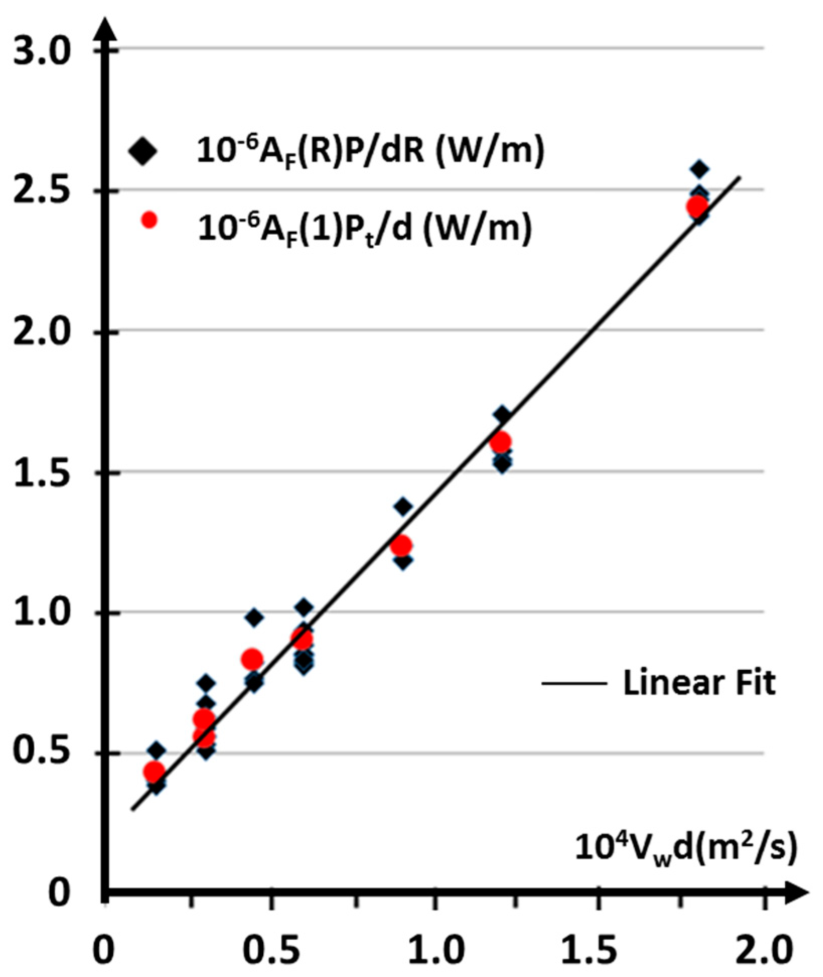
Knowing the dependence of P_t defined in the case of macro-welding (see Equation (6)), it is tempting to plot the variation of the similar variable A_F(1)P_t(d, V_w)/d, as a function of (V_wd): in fact, a linear dependence fits these data accurately (Figure 5), which is given by the relation:

$$\frac{{\mathrm{A}}_{\mathrm{F}}\left(1\right){\mathrm{P}}_{\mathrm{t}}\left(\mathrm{d},{\mathrm{V}}_{\mathrm{w}}\right)}{\mathrm{d}}={\mathrm{a}}_1+{\mathrm{b}}_1\left({\mathrm{V}}_{\mathrm{w}}\mathrm{d}\right),$$

(11)

In Equation (11), A_F(1) ≈ 0.32 is the Fresnel absorptivity for α = π/4, and the constants a₁ ≈ 2.1 x 10⁵ W/m and b₁ ≈ 1.2 x 10¹⁰ J/m³ can then be derived. Moreover, if one considers that a₁ ≈ n₁K(T_v – T₀) and b₁ ≈ m₁K(T_v – T₀)/(2.κ) similarly to in Equations (4) and (5), one then finds that: m₁ ≈ 2.1 and n₁ ≈ 2.2.

In fact, these values of m₁ and n₁ are rather close to the values of m and n observed in the case of a cylindrical KH. Indeed, they characterize the conductive losses of the geometry of this half-cone shape of the KH front used in this model. For similar reasons, it is also important to notice that the variable A_F(R)P/(dR), which can be estimated for any aspect ratio R and is also reported in Figure 5, follows the same scaling law with (V_wd). Accordingly, one can write:

$$\frac{{\mathrm{A}}_{\mathrm{F}}\left(\mathrm{R}\right)\mathrm{P}}{\left(\mathrm{dR}\right)}={\mathrm{a}}_1+{\mathrm{b}}_1\left({\mathrm{V}}_{\mathrm{w}}\mathrm{d}\right).$$

(12)

Using Equation (11), which defines the threshold P_t, Equation (12) can be simply rewritten as:

$$\mathrm{R}=\frac{{\mathrm{A}}_{\mathrm{F}}\left(\mathrm{R}\right)\mathrm{P}}{\mathrm{d}({\mathrm{a}}_1+{\mathrm{b}}_1\left({\mathrm{V}}_{\mathrm{w}}\mathrm{d}\right)}=\frac{{\mathrm{A}}_{\mathrm{F}}\left(\mathrm{R}\right)}{{\mathrm{A}}_{\mathrm{F}}\left(1\right)}\frac{\mathrm{P}}{{\mathrm{P}}_{\mathrm{t}}}.$$

(13)

Equation (13) shows that the inverse of the slope R/P is a linear function of the welding speed V_w, whose parameters depend of the spot diameter d (in agreement with Equation (10)).

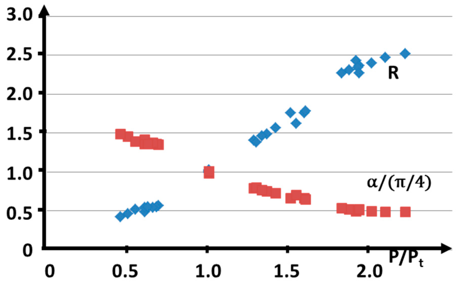
For the same set of operating parameters, the Figure 6 shows the evolution of the normalized inclination angle α/(π/4) and the evolution of R as a function of the normalized incident power P/P_t(d, V_w), where P_t(d, V_w) is the determined incident power threshold for any given d and V_w. These data follow unique curves, which can be easily understood because both α = Arctg(1/R), given by Equation (8), and R, through Equation (13), depend on P/P_t. The Fresnel absorptivity A_F(R) is also involved in these equations, but in the range of the aspect ratio used, the corresponding variation of A_F(R) is rather small: 0.31 < A_F(R) < 0.36.

Finally, one must notice that Equations (13) and (7) are very similar. They only differ by the expressions of the absorptivity and the corresponding power thresholds involved for each geometry.

Remark: For the derivation of Equation (13), it is supposed that there is no threshold for the process of melt pool surface depression, but this surface depression begins only if the velocity of the ejected melt V_m ≥ 0. From Equation (A10), this is only possible if the temperature exceeds a threshold temperature T_th, for which a threshold power P* is then determined by the model. One observes that P* increases with the spot diameter d. Therefore, taking into account this threshold power P*, Equation (13) should be modified as follows:

$$\mathrm{R}=\frac{{\mathrm{A}}_{\mathrm{F}}\left(\mathrm{R}\right)\left(\mathrm{P}-{\mathrm{P}}^{*}\right)}{{\mathrm{A}}_{\mathrm{F}}\left(1\right){\mathrm{P}}_{\mathrm{t}}},$$

(14)

The speed V_m of the ejected melt on the sides of the inclined KH front is another important parameter that characterizes this dynamic regime compared to the “thermal” one. On Figure 7, the parameter ΔV_m/V_w = (V_m/V_w − 1), which represents the variation of the melt ejection speed compared to the welding speed, has been plotted as a function of the three welding speeds V_w and the three spot diameters used, inside the range of the aspect ratios varying from 0.5 to 2.5.

It can be seen that ΔV_m/V_w increases quite linearly with the spot diameter d and more rapidly with the welding speed V_w. Additionally, for a given d and V_w, ΔV_m/V_w increases with the aspect ratio R. This ejected melt velocity can be very high compared to the welding speed when this welding speed or the spot diameter becomes important.

The evolution of ΔV_m/V_w can be understood by using the mass conservation equation (Equation (A2)) where one neglects the evaporation mass rate (which is negligible in mass rate, but not in corresponding involved absorbed power, see below) compared to the melted one. From Equation (A2), one easily obtains in that case:

$$\frac{{\mathsf{\Delta }\mathrm{V}}_{\mathrm{m}}}{{\mathrm{V}}_{\mathrm{w}}}=\left(\frac{{\mathrm{V}}_{\mathrm{m}}}{{\mathrm{V}}_{\mathrm{w}}}-1\right)\approx 0.5\left(\frac{\mathrm{d}}{{\delta }_0}\right),$$

(15)

The decrease of the melt thickness δ₀, (given by Equation (A1)), explains the observed behavior of ΔV_m/V_w: For example, δ₀ decreases when the surface temperature T_s increases (thanks to the increases the drilling speed V_d), which then increases the aspect ratio R (at a given welding speed V_w). Additionally, for a given spot diameter d and aspect ratio R (that defines α), the reduction of δ₀ results in an increase in welding speed V_w that increases V_d.

It is also instructive to analyze how the absorbed laser power is shared between the conductive losses, the melting process and the vaporization process. First, it can be seen that the absorbed power fractions devoted to these three processes, % P_cond, % P_fus and % P_vap, respectively, are fairly similar in this dynamic regime. However, some trends can be observed on the studied range of parameters: for example, when the diameter d increases, the tendency shows that % P_cond decreases from about 45% to 30%, while % P_vap increases from 20 to 35% and % P_fus is roughly constant about 30–35%. Additionally, for a given spot diameter d, % P_cond decreases from 40% to 30%, % P_fus increases from 30% to 40% and % P_vap is about 30%, with the increase of the welding speed V_w. Finally, the effect of an increase of the incident power P (that increases the aspect ratio R) results in rather small variations of % P_cond (from about 30 to 35%), of % P_vap (from 30 to 25%) and of % P_fus (about 35%).

3.4. Example of Application of This Model to the Analysis of Experiments on Ti-6Al-4V

Cunningham et al. [21] have recently published a rather large set of experiments on Ti-6Al-4V material for welding speeds varying from 0.4 to 1.2 m/s and incident laser powers from 100 to 500 W. They used a Gaussian distribution of laser intensity, characterized by a laser spot diameter at 1/e² maximum intensity of 95 µm. This intensity distribution is different from the uniform one used in the present GPM. Therefore, a smaller laser spot diameter d₀, typically defined at about half maximum intensity, should be used instead, which for this Gaussian distribution would correspond to approximately 56 µm.

Their measured penetration depth variation e, as a function of the incident power P, appears to have a linear scaling with incident power P above a threshold P’ of about 90 W:

$$\mathrm{e}\left(\mathrm{m}\right)\approx \mathrm{S}\left(\mathrm{P}-{\mathrm{P}}^{\prime }\right)\approx \left(\frac{\mathrm{k}}{{\mathrm{V}}_{\mathrm{w}}}\right)\left(\mathrm{P}-{\mathrm{P}}^{\prime }\right),$$

(16)

The slope S decreases with the welding speed V_w and by analyzing their published data, one finds that the slope variation S with the welding speed can be fitted by the hyperbolic relation: S ≈ k/V_w, with k ≈ 0.6–0.7 10⁻⁶ m²/J. Using Equation (13), this would mean that these experiments are realized in the range of high V_w of this dynamic regime, for which b₁(V_wd) > a₁. Indeed, this is the case for their operating parameters, so Equation (14) becomes:

$$\mathrm{e}\approx \frac{{\mathrm{A}}_{\mathrm{F}}\left(\mathrm{R}\right)\left(\mathrm{P}-{\mathrm{P}}^{*}\right)}{\left({\mathrm{b}}_1{\mathrm{V}}_{\mathrm{w}}\mathrm{d}\right)},$$

(17)

By comparing Equations (16) and (17), one has the same slope if k ≈ A_F(R)/b₁d. This implies that a spot diameter d ≈ 40 µm (by using A_F(R) ≈ 0.31, k ≈ 6.5 x10⁻⁷ m²/J and b₁ ≈ 1.2 x 10¹⁰ J/m³). Considering the approximation made on b₁ (through the uncertainty on m₁, K and κ), this derived value of d seems in a quite reasonable agreement with the expected one of 56 µm defined at half maximum intensity of the Gaussian intensity distribution. (In fact, Cunningham et al. [21] used a similar spot diameter (≈ 50 µm) for the discussion of their results).

As a conclusion of this section, it is shown that Equations (14) and (11), which define the aspect ratio R and the incident power threshold P_t respectively, as a function of the operating parameters and mean thermophysical properties of the used material, are representative solutions of this GPM which describes this dynamic welding regime where the inclined KH front is mainly irradiated, and KHs with rather low aspect ratios result. Despite the differences in the various physical mechanisms involved in these two models describing these two very distinct welding regimes, in particular, the importance of evaporation processes in the second model, it appears that the resulting scaling laws are almost identical, thereby explaining our previous finding that the penetration depths for the additive manufacturing processes followed the same scaling laws [19].

4. Analysis of KH Stability Near Its Threshold Around R ≈ 1

4.1. KH Absorptivity Variations

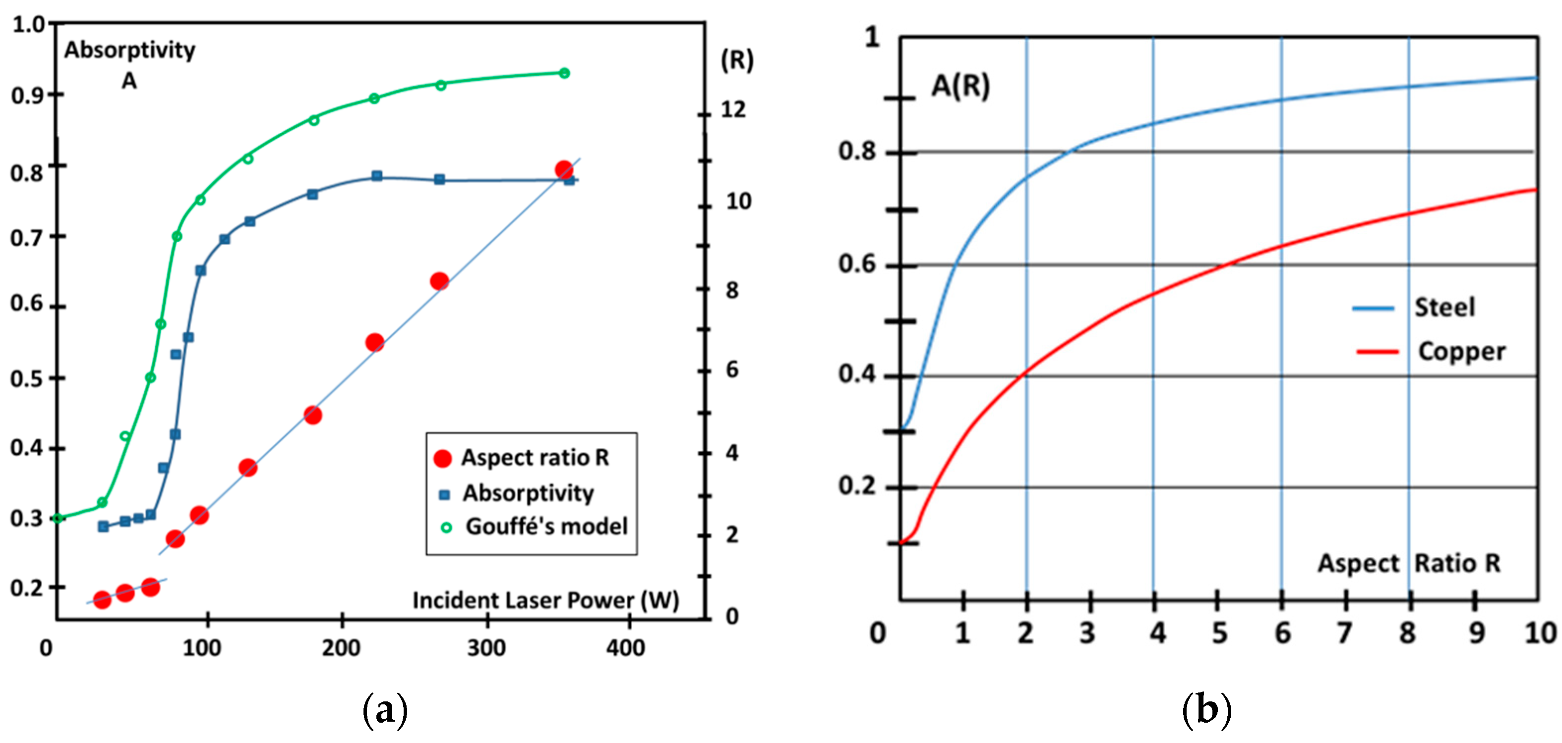
In the previous equations, one sees that the absorptivity A(R) of a KH is a determining parameter that controls the resulting aspect ratio R, and therefore, it must be known for any R. For a rather wide range of aspect ratios, the KHs absorptivity has been measured [30,31]. For example, Trapp et al. [30] realized calorimetric time integrated measurements on SS 316L steel. In Figure 8a, an example of their measured absorptivity for a welding speed of 0.5 m/s has been reproduced with the corresponding aspect ratio. A clear transition occurs at KH threshold when R ≈ 1. For comparison, for each aspect ratio R, the corresponding absorptivity using the Gouffé’s model [32] of beam trapping inside a cone-shape geometry (with A₀ ≈ 0.31) has been also reported. If the general trend is relatively well reproduced, we can nevertheless see that Gouffé’s model overestimates the absorptivity, and the transition around R = 1, which is quite different from the one observed experimentally. These deviations must mainly result from the difference in geometry between the real KH and the cone shape used in the Gouffé’s model.

In fact, if one considers the geometry of KH when R < 1, A(R) is rather well known, because of the well-defined KH front geometry that allows for the use of the Fresnel equations. But when R > 1, because the reflected beam is directed downwards and then the multiple reflections process starts, A(R) should increase and the total absorptivity of the KH should be higher than that given by the Fresnel equation, and this discrepancy increases with the aspect ratio.

Now for 1 < R < 2–3, the reflected beam from the KH front is not very strongly deflected downwards [29]; it is quite horizontal and it irradiates the KH rear wall, the height of which is equivalent to that of the KH front. (See for example, numerical simulations of Martin et al. [33]). But the effect of this interaction on the KH rear wall depends of the location of this wall, which is defined by the length of the KH aperture itself controlled by the welding speed. At high welding speed, as the melt ejection velocity V_m is high (see Figure 7), the KH is elongated and its geometry is controlled by this high melt velocity, and the KH aperture is then much larger than the focal spot (confirmed by X-ray radiographies of the KH at these high welding speeds [21,22]). This is a regime where humping is likely to start in the melt flow behind the KH. As a consequence, for this elongated KH, the interaction of the reflected beam with the KH rear wall does not modify its overall depth or the KH geometry, which is then stable.

But at low welding speed, the KH aperture is quite circular with a dimension of the order of the spot diameter. Therefore, when R begins to be greater than one, the interaction of the reflected beam on this rather close KH rear wall increases the overall absorptivity of the incoming laser beam. Typically, for these conditions, after this second interaction of the incoming beam, if one considers that the reflected beam exits from this KH aperture (because of some inclination of the KH rear wall towards the rear melt pool due to the melt flow [33]), the total absorptivity after these two reflections would be 1 − (1 − A₀)², where A₀ is a characteristic absorptivity of the melted KH surface. Then from there, if R continues to increase, the KH absorptivity increases further due to the increasing number of multi-reflections. Therefore, it is only inside a transition region located around R = 1 that A(R) cannot be clearly defined; however, one can expect that A(R) increases from A_F(1⁻), (when R is slightly lower than 1), which is typically given by the Fresnel absorptivity for α = π/4, and ends up joining an absorptivity close to the Gouffé’s absorptivity A_G(1⁺) (when R is slightly greater than 1). The effects of these possible variations of A(R) inside this transition zone on the KH stability are discussed now.

4.2. Dependance of the KH Front Inclination for a Given Incident Laser Power

We have previously seen that both regimes can be described by an equation similar to Equation (13) that relates the aspect ratio R as a function of incident power P, the corresponding absorptivity A(R) and the power threshold A(1)P_t ≈ d(a + b(V_wd)). But because rather similar parameters a and b have been obtained for both regimes, for the sake of simplicity, we will assume the same power threshold A(1)P_t in what follows. Therefore, for a given incident power P, the resulting aspect ratio R will then be a solution to Equation (18):

$$\frac{\mathrm{R}}{\mathrm{A}\left(\mathrm{R}\right)}=\frac{\mathrm{P}}{\mathrm{A}\left(1\right){\mathrm{P}}_{\mathrm{t}}}={\mathrm{P}}_{\mathrm{n}},$$

(18)

In Equation (18), a normalized incident power P_n = P/(A(1)P_t) has been defined.

For a given incident normalized power P_n, we have examined the solution of Equation (18) by using three different variations of A(R) around R = 1. These three cases are reported on Figure 9a. They all have the same constant absorptivity A₀ from for 0 < R < 1⁻. The first one considers a discontinuous (non-realistic) variation at R = 1 from A₀ to A_G(1) (A_G(1) is given by the Gouffé’s model for R = 1). The two others show more realistic evolutions, with a continuous transition being rather sharp (red curve) or smooth (green curve) for 1⁻ < R < 1⁺. For R > 1⁺, these three variations follow the Gouffé’s model of absorptivity A_G(R). The corresponding evolutions of R/A(R) have been reported on Figure 9b, and different values of P_n have been considered.

In the case of the discontinuous variation of A(R) (blue curves in Figure 9), it is easy to see that R/A(R) varies linearly from 0 to 1/A₀ for 0 < R <1. For R > 1, it increases quite linearly from 1/A_G(1) with a slope locally defined by the Gouffé’s model. One can see that the discontinuity of A(R) at R = 1 induces for R/A(R) two separate branches on each side of R = 1. Therefore, if P_n < 1/A_G(1) or P_n > 1/A₀, there is a unique solution of Equation (18) for R. However if 1/A_G(1) < P_n < 1/A₀, two solutions for R are obtained: one being such that R₁ < 1, and for the other one, R₂ >1 (see Figure 9a). One must note that these two solutions are physically possible because they both correspond to positive derivatives of R with incident power P_n.

In order to estimate the corresponding normalized incident power P/P_t instead of P_n, we assume here that A(1) ≈ 1 − (1 − A₀)² = 0.52, which would be the KH absorptivity when only two reflections occur inside (see Figure 2c). Therefore, the previous power ranges can be also written as (for steel):

-

For P/P_t < (P/P_t)_min = A(1)/A_G(1) ≈ 0.8, only one solution with R < 1 is obtained, which does not correspond to a KH. It can be considered as some “forced” conductive regime, where the melt pool surface is depressed with an inclination angle α > π/4.

-

For P/P_t > (P/P_t)_max = A(1)/A₀(≈1.7), only one solution also exists for R such that R > R_max ≈ 2.6 (with R_max being the solution of A₀R_max=A_G(R_max)).

-

For (P/P_t)_min < P/P_t < (P/P_t)_max, two solutions, R₁ and R₂, are such that R_min = A₀/A_G(1)(≈0.5) < R₁, R₂ < R_max.

In fact, it is tempting to consider that for this discontinuous variation of A(R), these two solutions for R, obtained in the power range ≈0.8 < P/Pt < ≈1.7, are representative of some unstable regime that could occur on the KH front. Indeed, as these two solutions are physically possible, there is no reason that the KH is stabilized on only one solution, because the melt KH surface is not static; it is a moving fluid with ripples on its surface [34], so switching from one geometry to another is quite possible.

Now, if one considers the effect of the second type of A(R) variation, which has a continuous but rather sharp transition at R = 1 (red curves in Figure 9), one can see that R/A(R) shows a decreasing part located between a maximum and a minimum located on either side of R = 1. But for the same reason as previously, this decreasing part is not physically possible because it would correspond to an increase of the aspect ratio when the incident power decreases. Therefore again, two solutions for R would be possible for a given range of normalized power P_n, but now inside a reduced range compared to the first case.

Finally, for the third type of A(R) variation with a smoother transition around R = 1 (green curves, in Figure 9), one observes that R/A(R) is always a monotonous increasing function. Therefore, only one solution for R can be obtained, which means that a stable geometry of the KH front is obtained for any value of the incident power P_n.

This model-based approach of the effect of the absorptivity variation around R = 1, seems to show that a stable KH front geometry is unlikely for these conditions. Due to the fact that the corresponding real variation of A(R) is rather unknown, in order to avoid this unstable zone, the use of incident powers P high enough in order to obtain aspect ratios R greater than about R_max (≈2 for steel) seems recommendable.

One can also add that the range of P/P_t that corresponds to the instable behavior is also dependent of the absorptivity A₀ of the used material. For example, by using the same discontinuous variation model of A(R), inside the “unstable” zone, one can compare the ranges of P/P_t and the corresponding solutions R₁ and R₂ for copper (with A₀ ≈ 0.1) and for steel (with A₀ ≈ 0.31) (it should be recalled, however, that more realistic conditions for A(R) should of course show narrower ranges). For steel, we have seen that 0.8 < P/P_t < 1.7 with R₁, R₂ varying from 0.5 to 2.6. For copper, (with A₀ ≈ 0.10), one obtains 0.6 < P/P_t < 1.9, but with R₁, R₂ varying from 0.35 to 6.5. Therefore, one sees that the resulting range for the variations of R₁ and R₂ is enlarged when the material absorptivity decreases, and higher laser power is required to enter in the stable KH regime. It is interesting to notice that Heider’s experiments on copper welding [27], clearly show that only high incident laser powers, which generate deep KHs, produce high quality welds. A possible consequence of this result would be to consider that any increase of the absorptivity, either by using materials with higher absorptivities or by using shorter laser wavelengths, should improve the stability of the KH front for these operating conditions.

4.3. Experimental Observation of These Unstable Behaviors

4.3.1. Welding Experiments

In order to test the prediction of our model of the occurrence of some unstable behavior around the KH threshold P_t, a set of very simple experiments has been undertaken. In order to cover the conduction to the KH modes, weld seams have been realized for different incident laser powers, at several welding speeds. A continuous-wave laser light with a wavelength of 1.03 µm was used, with a uniform beam intensity distribution inside a spot size of 600 µm diameter. The melt pool was also observed with a PHOTRON Fastcam high speed video camera at 10 kHz frame rate. One expects that this unstable regime is characterized by some fluctuations of the melt pool that could lead to some melt ejection, and therefore, to the occurrence of blow-holes inside the weld seam. Therefore, the number of blow-holes that appeared along the weld seam track should be an indicator of the stability of the welding process. For a welding speed V_w = 1 m/min, Figure 10 shows the number of blow-holes observed along a 45 mm bead length on mild steel, as a function of the incident laser power. It is remarkable to notice that these blowholes appear only within a range of laser powers extending from 400 to 1000 W. Additionally, the corresponding depths of these blow-holes have been reported.

Finally, the corresponding threshold laser power P_t can be estimated by using Equations (5) and (6), and the evaluation of the constants a and b. This kind of determination is fairly approximate, because there is a rather large uncertainty on the different involved thermophysical parameters. However, for mild steel, by using the following thermophysical data: ρ ≈ 7800 kg/m³, C_p ≈ 800 J/kgK, K ≈ 30 W/mK, T_v ≈ 3100 K, T₀ ≈ 300 K, one finds that a ≈ 2.5 × 10⁵ W/m and b ≈ 2 × 10¹⁰ J/m³. The constants m and n used are those involved in the thermal model; typically, m ≈ 2.4 and n ≈ 3, and A(1) is about 0.6.

As a result, with these parameters one finds that P_t ≈ 450 W for a welding speed V_w = 1 m/min, and if one uses the previous range of 0.8 < P/P_t < 1.7 for the critical zone, it would correspond for our conditions to 360 W < P < 765 W, which is in a surprising agreement with the experimental power range where blow-holes are observed.

High speed videos of a sequence leading to the occurrence of this blow-hole show that the melt pool surface is first lifted and then explodes, leaving a blow-hole behind the melt pool. One interpretation would be that the interaction of the metallic vapor ejected perpendicularly from the KH front with the melt pool plays an important role in the complex dynamics of the melt pool [28,35]. For these operating conditions, as the KH front inclination should be around 45° and with the rear KH wall being rather close, this vapor jet leaving the KH front could penetrate inside the liquid KH rear wall and cause the observed lifting of the melt pool. But if this effect should occur here, it should be also accompanied by the emission of spatters usually observed to be ejected from the KH rim, which was not seen at all. Therefore, the effect of this vapor jet, if it cannot be completely excluded, may not be entirely satisfying to explain the observed dynamics of the melt pool.

The multi-physics simulations of Martin et al. [33] that take into account ray-tracing of the laser beam propagation inside the KH, show that due to this multi-reflections process, the rear KH wall can be directly irradiated by the reflected beam from the KH front wall when its inclination is about 45°. The resulting recoil pressure on this rear wall of the KH prevents the KH from closing due to surface tension and controls the position of the rear wall. However, this rear wall is subject to many fluctuations due to this unstable balance of the inner geometry of the KH, which is controlled by the distribution of the surface tension pressure and the recoil pressure resulting from these multi-reflections.

These simulations were realized for operating conditions of additive manufacturing (V ≈ 0.8 m/s, spot diameter d ≈ 50 µm), where the KH length is rather elongated (about 250 µm) and strongly fluctuates inside the melt pool of about 600 µm length (see an example in Figure 11a). These conditions are of course very different from the ones we used. But this mechanism could also be applied to our conditions, and it is possible to propose another scenario based on multi-reflections for explaining the previous experimental results.

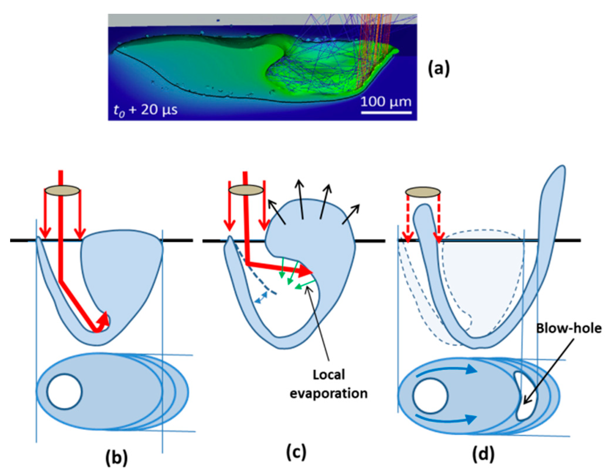
One starts with a given incident laser power that is high enough to generate a corresponding KH of low aspect ratio, (typically R ≈ 1–2); therefore, with an inclination angle lower than π/4 (Figure 11b). At some point, probably due to fluctuations within the melting front we have seen that for the same operating conditions, the inclination of the KH front can be switched to the other solution described in Section 4.1 for which R < 1, and thus an inclination α > π/4 exists. This incident laser power which is capable of generating the KH inside the solid sample is therefore suddenly mainly redirected toward the melt (Figure 11c). A strong evaporation must therefore occur locally at the impact, as the video shows that the melt pool surface rises in a few milliseconds, like a bubble, which eventually bursts, but with practically no loss of melt through this ejection. Then, the melt returns to the inside of the cavity thus produced, and during the reorganization of this melt—the laser beam being ever-present and continuing to move forward—a blow-hole is then left on the rear side of the melt pool (Figure 11d). It is obvious that the use of a time-resolved X-ray radiography would be much more appropriate to visualize the internal geometry of this liquid bubble during its expansion.

These experiments have been reproduced at welding speeds of 5 and 9 m/min with higher incident laser powers varying from 0.5 to 10 kW, (the corresponding power thresholds P_t being estimated respectively to 1250 and 2000 W). In fact, no significant appearance of similar blow-holes was observed in these cases. Because of these higher welding speeds and the large focal spot diameter used here, the velocity of the melt ejected backwards is higher than at V_w = 1 m/min, and consequently makes the KH aperture appear rather elongated, particularly for V_w = 9 m/min. Moreover, for these high welding speeds, the width of the melt pool is narrower; this geometry should be therefore less prone to being lifted by the reflected beam. Therefore, this result seems to confirm that this unstable regime should mainly occur when the KH rear wall is rather close to the KH front, and more generally, when the velocity of ejected melt backwards is low (see corresponding conditions on Figure 7).

4.3.2. Spot-Welding Experiments

The previous absorptivity measurements, based on time-integrated measurements with calorimetry techniques, are not representative of the time-dependent variations of the absorptivity that should occur inside the KH for R ≈ 1. We have seen that these two solutions R₁ or R₂ are obtained when an absorptivity A(R₁) or A(R₂) of about A₀ and A_G(1) respectively occurs. Only time-dependent measurement of the absorptivity, obtained for example by measuring the reflected laser power from the sample by using an integrating sphere, can be suitable to follow its evolution. This technique has been employed by Simmonds et al. [36], but during a “spot welding” (SP) process, where the welding speed V_w = 0, so the sample was irradiated locally in a pulsed mode in order to generate a weld nugget. In fact, one can also apply the previous scheme of KH formation by considering that there is also a threshold for generating the keyhole for these static conditions. Indeed, when the melt pool surface with a cylindrical symmetry is depressed from the beginning of the interaction, its inclination also decreases, and the reflected beam that was initially reflected upwards is gradually deflected downwards and can be refocused downwards on its axis, when the mean inclination of the melt pool surface becomes greater than π/4. It then follows that the depression increases sharply and oscillates (similar conditions have also been visualized using coherent X-ray radiography by Cunningham et al. [21]), and leads to generating a deep KH that induces an increase of the absorptivity [37].

Experimentally, by using an integrating sphere, the time dependence of the reflected beam was measured for different incident laser powers, and a power threshold P_t-SP (defined such that the melt pool depth equals the spot diameter) has been estimated [36]. As expected, for P < P_t-SP, the absorptivity of the melt pool surface is constant at about 0.30, and for P > P_t-SP, because of the multiple reflections inside the increasing depth of the cylindrical KH, the absorptivity increases with the incident laser power while remaining stable. But for P ≈ P_t-SP, the time-dependent absorptivity during the pulse duration shows several humps where the absorptivity varies from about 0.30 (the typical absorptivity of the melt pool surface) to about 0.50 (some absorptivity of a non-completely developed KH). The time interval between the observed oscillations peaks of absorptivity probably corresponds to the delay for achieving the maximum penetration of the KH that follows its closure due to the surface tension effect. One can understand that for these threshold conditions, the intensity distribution at the bottom of the depression that controls the recoil pressure, which roughly equilibrates the local surface tension pressure, can be easily perturbed by the unavoidable fluctuations of the KH surface.

Experimentally, the threshold seems to appear for an incident pulse energy range from ≈2 J to ≈2.9 J, delivered with a pulse duration of 10 ms, which corresponds to a power range ≈200 W < P < ≈290 W. But these experiments that use a short pulse duration are not characteristic of a stationary regime. Nevertheless, for a rough estimation of the corresponding threshold, and to compare it with the experimental one, Equation (6) could be used in the limiting case of low welding speeds V_w, which would give P_t ≈ ad/A(1). The parameter a = nK(T_v − T₀) is evaluated using the 316 L material properties utilized for these experiments [36]. With n ≈ 3, K ≈ 30 W/mK, T_v = 3300 K, T₀ = 300 K; a spot diameter of 300 µm (with uniform intensity distribution); and using A(1) ≈ 0.6, one obtains P_t = ad/A(1) ≈ 135 W, which is about half the value obtained experimentally. Despite this observed difference, given the various uncertainties associated with the estimation of the parameters a or A(1), and more particularly in the experimental determination of the threshold power (which in fact must depend on the pulse duration used, decreasing as the pulse duration increases), this approach can nevertheless be considered appropriate, as it confirms the unsteady nature of the keyhole absorptivity near its threshold.

5. Conclusions

Several issues addressed in this study concern the analysis of the KH behavior for different regimes of laser welding used in several industrial applications: These processes cover deep KHs with large aspect ratios obtained at low welding speeds with multi-kilowatt lasers, and those with much smaller aspect ratios, realized at high welding speeds, with small focal spots and lasers with low incident power. One important issue is about the determination of the scaling law of the resulting aspect ratios for these very different operating conditions.

By using a generalized piston model, it has been shown that the scaling laws obtained in the case of the “thermal” model applied to low welding speeds or high aspect ratios, can be formally extended to operating conditions where the laser absorption occurs mainly on the inclined absorbing KH front, which are characteristic of high welding speed processes or low aspect ratios.

This generalized piston model has allowed us to study the behavior of several parameters of the ejected melt flow and to define the threshold conditions for KH formation, when the aspect ratio is equal to one. Moreover, it has been shown that operating parameters around this threshold should induce unstable behavior of the rear KH wall, and therefore defects in the resulting weld seam at low welding speeds. Therefore, experimental observations could be explained by this mechanism.

As a more general result of this study, it could be proposed that a necessary condition for obtaining a stable laser welding process in the KH mode would be to generate KHs with fairly high aspect ratios, above a specified limit, this limit being dependent on the laser absorptivity of the material. It would increase as this laser absorptivity decreases. This tendency also seems to be verified when comparing laser welding of copper alloys or steels. Furthermore, it is known that weld seams obtained by the laser power bed fusion process have rather low aspect ratios, which could make them sensitive to this kind of instability as well.

In the same vein, it can be also concluded that the use of a short laser wavelength (green or blue) which strongly increases the absorptivity of any material—and thus decreases the effect of multi-reflections within the KH—should be an efficient way to easily reduce the range of the operating parameters leading to process instability. Future experiments in this direction are of course highly expected.

References

- Gu, D.D.; Meiners, W.; Wissenbach, K.; Poprawe, R. Laser additive manufacturing of metallic components: Materials, processes and mechanisms. Int. Mater. Rev. 2012, 57, 133–164. [Google Scholar] [CrossRef]
- Yap, C.Y.; Chua, C.K.; Dong, Z.L.; Liu, Z.H.; Zhang, D.Q.; Loh, L.E.; Sing, S.L. Review of selective laser melting: Materials and applications. Appl. Phys. Rev. 2015, 2, 041101. [Google Scholar] [CrossRef]
- Rosenthal, D. The theory of moving sources of heat and its application to metal treatments. Trans. ASME 1946, 68, 849–866. [Google Scholar]
- Swift-Hook, D.T.; Gick, A.E.F. Penetration welding with lasers. Weld. Res. Suppl. J. 1973, 52, 492–499. [Google Scholar]
- Dowden, J.; Postacioglu, N.; Davis, M.; Kapadia, P. A keyhole model in penetration welding with a laser. J. Phys. D Appl. Phys. 1987, 20, 36–44. [Google Scholar] [CrossRef]
- Noller, F. The stationary shapes of vapor cavity and molten zone in EB-welding. In Proceedings of the 3rd CISFFEL, International Colloquium on Welding and Melting by Electrons and Laser Beam, Lyon, France, 5–9 September 1983; pp. 89–97. [Google Scholar]
- Kroos, J.; Gratzke, U.; Simon, G. Towards a-self-consistent model of the keyhole in penetration laser beam welding. J. Phys. D Appl. Phys. 1993, 26, 474–480. [Google Scholar] [CrossRef]
- Kaplan, A. A model of deep penetration laser welding based on calculation of the keyhole. J. Phys. D Appl. Phys. 1994, 27, 1805–1814. [Google Scholar] [CrossRef]
- Sudnik, D.; Radaj, D.; Erofeew, W. Computerized simulation of laser beam welding, modelling and verification. J. Phys. D Appl. Phys. 1996, 29, 2811–2817. [Google Scholar] [CrossRef]
- Ki, H.; Mohanty, P.S.; Mazumder, J. Modeling of laser keyhole welding: Part I. Mathematical modeling, numerical methodology, role of recoil pressure, multiple reflections, and free surface evolution. Metall. Mater. Trans. A 2002, 33, 1817–1830. [Google Scholar] [CrossRef]
- Geiger, M.; Leitz, K.H.; Koch, H.; Otto, A. A 3D transient model of keyhole and melt pool dynamics in laser beam welding applied to the joining of zinc coated sheets. Prod. Eng. 2009, 3, 127–136. [Google Scholar] [CrossRef]
- Pang, S.; Chen, L.; Zhou, J.; Yin, Y.; Chen, T. A three-dimensional sharp interface model for self-consistent keyhole and weld pool dynamics in deep penetration laser welding. J. Phys. D Appl. Phys. 2011, 44, 025301. [Google Scholar] [CrossRef]
- Courtois, M.; Carin, M.; Masson, P.; Gaied, S.; Balabane, M. A new approach to compute multi-reflections of laser beam in a keyhole for heat transfer and fluid flow modelling in laser welding. J. Phys. D Appl. Phys. 2013, 46, 505305. [Google Scholar] [CrossRef]
- Tan, W.; Shin, Y.C. Analysis of multi-phase interaction and its effects on keyhole dynamics with a multi-physics numerical model. J. Phys. D: Appl. Phys. 2014, 47, 345501. [Google Scholar] [CrossRef]
- Zhao, H.; Niu, W.; Zhang, B.; Lei, Y.; Kodoma, M.; Ishide, T. Modelling of keyhole dynamics and porosity formation considering the adaptive keyhole shape and three-phase coupling during deep-penetration laser welding. J. Phys. D Appl. Phys. 2011, 40, 5753–5766. [Google Scholar] [CrossRef]
- Fabbro, R.; Dal, M.; Peyre, P.; Coste, F.; Schneider, M.; Gunenthiram, V. Analysis and possible estimation of keyhole depths evolution, using laser operating parameters and material properties. J. Laser Appl. 2018, 30, 032410. [Google Scholar] [CrossRef]
- Rubenchick, A.M.; King, W.E.; Wu, S.S. Scaling laws for additive manufacturing. J. Mater. Process. Technol. 2018, 257, 234–243. [Google Scholar] [CrossRef]
- King, W.E.; Barth, H.D.; Castillo, V.M.; Gallegos, G.F.; Gibbs, J.W.; Hahn, D.E.; Kamath, C.; Rubenchik, A.M. Observation of keyhole-mode laser melting in laser powder-bed fusion additive manufacturing. J. Mater. Process. Technol. 2014, 214, 2915–2925. [Google Scholar] [CrossRef]
- Fabbro, R. Scaling laws for the welding process in keyhole mode. J. Mater. Process. Technol. 2019, 264, 346–351. [Google Scholar] [CrossRef] [Green Version]
- Berger, P.; Hügel, H. Fluid dynamic effect in keyhole welding – an attempt to characterize different regimes. Phys. Procedia 2013, 41, 216–224. [Google Scholar] [CrossRef] [Green Version]
- Cunningham, R.; Zhao, C.; Parab, N.; Kantzos, C.; Pauza, J.; Fezzaa, K.; Sun, T.; Rollett, A.D. Keyhole threshold and morphology in laser melting revealed by ultrahigh-speed x-ray imaging. Science 2019, 363, 849–852. [Google Scholar] [CrossRef]
- Kouraytem, N.; Li, X.; Cunningham, R.; Zhao, C.; Parab, N.; Sun, T.; Rollett, A.D.; Spear, A.D.; Tan, W. Effect of Laser-Matter Interaction on Molten Pool Flow and Keyhole Dynamics. Phys. Rev. Appl. 2019, 11, 064054. [Google Scholar] [CrossRef]
- Semak, V.; Matsunawa, A. The role of recoil pressure in energy balance during laser materials processing. J. Phys. D Appl. Phys. 1997, 30, 2541–2552. [Google Scholar] [CrossRef]
- Lankalapalli, K.N.; Tu, J.T.; Gartner, M. A model for estimating penetration depth of laser welding processes. J. Phys. D Appl. Phys. 1996, 29, 1831–1841. [Google Scholar] [CrossRef]
- Miyazaki, T.; Giedt, W.H. Heat transfer from an elliptical cylinder moving through an infinite plate applied to electron beam welding. Int. J. Heat Mass Transf. Theory Appl. 1982, 25, 807–814. [Google Scholar]
- Suder, W.J.; Williams, S. Power factor model for selection of welding parameters for CW laser welding. Opt. Laser Technol. 2014, 56, 223–229. [Google Scholar] [CrossRef]
- Heider, A.; Stritt, P.; Weber, R.; Graf, T. High power laser sources enable high-quality laser welding of copper. In Proceedings of the ICALEO Conference, San Diego, CA, USA, 19–23 October 2014; pp. 343–348. [Google Scholar]
- Fabbro, R. Melt pool and keyhole behavior analysis for deep penetration laser welding. J. Phys. D Appl. Phys. 2010, 43, 445501. [Google Scholar] [CrossRef]
- Fabbro, R.; Chouf, K. Keyhole modeling during laser welding. J. Appl. Phys. 2000, 87, 4075. [Google Scholar] [CrossRef]
- Trapp, J.; Rubenchik, A.M.; Guss, G.; Matthews, M.J. In situ absorptivity measurements of metallic powders during laser powder-bed fusion additive manufacturing. Appl. Mater. Today 2017, 9, 341–349. [Google Scholar] [CrossRef]
- Ye, J.; Khairallah, S.A.; Rubenchik, A.M.; Crumb, M.F.; Guss, G.; Belak, J.; Matthews, M.J. Energy Coupling Mechanisms and Scaling Behavior Associated with Laser Powder Bed Fusion Additive Manufacturing. Adv. Eng. Mater. 2019, 21, 1900185. [Google Scholar] [CrossRef]
- Gouffe, A. Correction d’ouverture des corps noirs artificiels compte tenu des diffusions multiples internes. Rev. Opt. 1945, 24, 1–10. [Google Scholar]
- Martin, A.A.; Nicholas, P.; Calta, P.; Joshua, A.; Hammons, J.A.; Khairallah, S.A.; Nielsen, M.H.; Shuttlesworth, R.S.; Sinclair, N.; Matthews, M.J.; et al. Ultrafast dynamics of laser-metal interactions in additive manufacturing alloys captured by in situ X-ray imaging. Mater. Today Adv. 2019, 1, 100002. [Google Scholar] [CrossRef]
- Kaplan, A.F.H.; Samarjy, R.S.M. Absorption peaks depending on topology of the keyhole front and wavelength. J. Laser Appl. 2015, 27, S29012. [Google Scholar] [CrossRef]
- Weberpals, J.-P. Nutzen und Grenzen Starker Fokussierung Beim Laserschweißen. Ph.D. Thesis, University of Stuttgart, Stuttgart, Germany, 2010. [Google Scholar]
- Simonds, B.J.; Sowards, J.; Hadler, J.; Pfeif, E.; Wiltham, B.; Tanner, J.; Harris, C.; Williams, P.; Lehman, J. Time-Resolved Absorptance and Melt Pool Dynamics during Intense Laser Irradiation of a Metal. Phys. Rev. Appl. 2018, 10, 044061. [Google Scholar] [CrossRef]
- Ki, H.; Mohanty, P.S.; Mazumder, J. Multiple reflection and its influence on keyhole evolution. J. Laser Appl. 2002, 14, 39–45. [Google Scholar] [CrossRef]
- Mas, C.; Fabbro, R.; Gouedard, Y. Steady state laser cutting modeling. J. Laser Appl. 2003, 15, 145–152. [Google Scholar] [CrossRef]
- Dausinger, F.; Shen, J. Energy coupling efficiency in laser surface treatment. ISIJ Int. 1993, 33, 925–933. [Google Scholar] [CrossRef] [Green Version]
- Knight, C.J. Theoretical modeling of rapid surface vaporization with back pressure. AIAA J. 1979, 17, 519–523. [Google Scholar] [CrossRef]
- Samokhin, A.A. First-order Phase Transitions Induced by Laser Radiation in Absorbing Condensed Matter; Effect of Laser Radiation on Absorbing Condensed Matter, Nova Science Publishers: Commack, NY, USA, 1990; pp. 1–161. [Google Scholar]
- Abe, Y.; Mizutani, M.; Kawahito, Y.; Katayama, S. Deep penetration welding with high power laser under vacuum. In Proceedings of the ICALEO, Anaheim, CA, USA, 26–30 September 2010; LIA, Ed.; pp. 648–653. [Google Scholar]
- Borner, C.; Dilger, K.; Rominger, V.; Harrer, T.; Krussel, T.; Lower, T. Influence of ambient pressure on spattering and weld seam quality in laser beam welding with the solid-state laser. In Proceedings of the ICALEO, Orlando, FL, USA, 23–27 October 2011; LIA, Ed.; pp. 621–629. [Google Scholar]
- Rominger, V.; Berger, P.; Hügel, H. Effects of reduced ambient pressure on spattering during the laser beam welding of mild steel. J. Laser Appl. 2019, 31, 042016. [Google Scholar] [CrossRef]
- Fabbro, R.; Hirano, K.; Pang, S. Analysis of the physical processes occurring during deep penetration laser welding under reduced pressure. J. Laser Appl. 2016, 28, 022427. [Google Scholar] [CrossRef] [Green Version]
Figure 1.
For different operating parameters (incident power P and spot diameters d), the plot of P/dR as a function of (Vwd), corresponding best linear fit using Equation (4) [19] (from data published by Suder and Williams [26]).
Figure 2.
Characteristic longitudinal profile of the keyhole (KH) fronts for different welding speeds. (a) At low welding speed, a KH with a high aspect ratio R is obtained due to multi-reflections inside it. (b) At high welding speed only the KH front is irradiated; the reflected beam is directed upwards. (c) At KH threshold, (R = 1), the reflected beam is horizontal and interacts with the KH rear wall. Corresponding views of the KH aperture (d = 0.6mm, P = 4 kW; 316L material) [28].
Figure 3.
Scheme of the half-cone shape of the KH front used for applying the GPM that describes the dynamic welding regime.
Figure 4.
Examples of the aspect ratio R dependence with the incident power P for different welding speeds Vw (a spot diameter d = 120 µm is used).
Figure 5.
Plot of AF(1)Pt/d and AF(R)Pt/dR as a function of (Vwd) and corresponding best linear fit.
Figure 6.
Variations of the normalized inclination angle of the KH front α/(π/4) and the aspect ratio R as a function of the normalized incident power P/Pt.
Figure 7.
Variation of ΔVm/Vw = (Vm/Vw − 1) for the three welding speeds Vw and the three spot diameters used, inside the range of the aspect ratios 0.5 < R < 2.5.
Figure 8.
(a) From Trapp et al. [30]: time integrated absorptivity of 316l SS steel as a function of incident power for a welding speed Vw = 0.5 m/s (blue squares); corresponding measured aspect ratios R = e/d0.5 (d0.5 ≈ 40 µm) (red dots). For each aspect ratio, the resulting absorptivity from the Gouffé’s model for a conical geometry has been reported (green dots). (b) Examples of absorptivity from the Gouffé’s model for a conical geometry (for steel, with A0 ≈ 0.31) and copper, with A0 ≈ 0.1).
Figure 9.
(a) Three examples of variation of the absorptivity A(R) around R = 1. Blue curve: discontinuous variation from A0 to AG(1) at R = 1. Red curve: smooth but rather sharp transition around R = 1. Green curve: much smoother transition. Dotted curve: Gouffé’s absorptivity for a cone (for steel, λ = 1.03 µm). (b) Corresponding evolutions of R/A(R) for these three cases of variation of the absorptivity. (A0 ≈ 0.31 for steel at λ = 1.06 µm is used, and AG(1) is the absorptivity given by the Gouffé’s law at R = 1).
Figure 10.
Number of blow-holes on a 45 mm bead length and depth of the blow-holes, as a function of the incident laser power (on mild steel material, 0.6 mm spot diameter; Vw = 1 m/min). Typical aspects of surface weld seams for these welding regimes: the conduction, unstable and KH regime.
Figure 11.
(a) Example of multi-physics simulations of the multi-reflections mechanism inside the KH [33]. Sequence of events leading to melt pool perturbation: (b) A low aspect ratio KH is first generated. (c) Due to fluctuations that modify the KH front inclination, the incident laser beam is redirected toward the melt pool whose surface is lifted and then tears; a transient cavity forms and then fills (d) A new melt pool is reconstructed but with a blow-hole left behind.
© 2020 by the author. Licensee MDPI, Basel, Switzerland. This article is an open access article distributed under the terms and conditions of the Creative Commons Attribution (CC BY) license (http://creativecommons.org/licenses/by/4.0/).
Share and Cite
MDPI and ACS Style
Fabbro, R. Depth Dependence and Keyhole Stability at Threshold, for Different Laser Welding Regimes. Appl. Sci. 2020, 10, 1487. https://doi.org/10.3390/app10041487
AMA Style
Fabbro R. Depth Dependence and Keyhole Stability at Threshold, for Different Laser Welding Regimes. Applied Sciences. 2020; 10(4):1487. https://doi.org/10.3390/app10041487
Chicago/Turabian StyleFabbro, Remy. 2020. "Depth Dependence and Keyhole Stability at Threshold, for Different Laser Welding Regimes" Applied Sciences 10, no. 4: 1487. https://doi.org/10.3390/app10041487
Note that from the first issue of 2016, this journal uses article numbers instead of page numbers. See further details here.