Simulation of Three Constitutive Behaviors Based on Nonlinear Ultrasound


State Key Laboratory of Power System, Department of Electrical Engineering, Tsinghua University, Beijing 100084, China
*
Author to whom correspondence should be addressed.
Appl. Sci. 2020, 10(6), 1982; https://doi.org/10.3390/app10061982
Submission received: 12 February 2020
/
Revised: 5 March 2020
/
Accepted: 6 March 2020
/
Published: 13 March 2020
(This article belongs to the Special Issue Nondestructive Testing (NDT))
Abstract
:Nonlinear ultrasound has attracted more and more attention. In classical acoustic nonlinear theory, the source of nonlinearity is the change of constitutive relation of materials. Structure response that distorts after a single tone ultrasound wave is important to detect imperfection. This is rarely found in current simulations. The current simulation always introduces defects which do not match to the classical acoustic nonlinear theory. In this manuscript, the recurrence expressions of three kinds of imperfect materials for subroutine are given. The verifying simulation model that is used for verifying recurrence equations and wave propagation model that are used for analysing the process of ultrasonic propagation are established. The results show that the two constitutive models are effective in the verifying simulation and the hysteresis material has some special characteristics. Finally, ultrasonic propagation in two types of materials produce the expected harmonics, which build foundations for simulations of nonlinear ultrasound.
1. Introduction
Under cyclic loads or harsh environments, no matter what materials, parts and complete structures will undergo material properties degradation. Continuous degradation leads to predictable and unpredictable problems, sometimes with serious consequences. Therefore, it is necessary to do health testing for structures or materials in practical engineering [1,2,3,4,5].
The early degradation of the mechanical properties takes up most of the life of the structures. Generally in metals, the damage first appears in the form of dislocation substructures such as veins and persistent slip bands (PSBs), and these accumulate at grain boundaries to produce strain localization and then further produce micro-cracks. This process accounts for 80–90% [6,7] of the life of the whole structure when the metal material structure is bearing a cyclic load or harsh environment. When the cracks show, the life the of material is almost over, so the testing of the early properties of the materials is particularly important.
With the development of ultrasonic non-destructive testing technology, linear ultrasound cannot satisfy the current testing needs, because linear ultrasound technology has no high sensitivity in the early stage of deterioration of material mechanical properties [8]. Studies show that the dislocation substructures and resulting microplastic deformation do not cause large changes in the macroscopic properties such as elastic modulus, sound speed and attenuation of a material [9,10], thus the changes in the linear ultrasonic quantities are not large enough to be accurately measured with conventional linear ultrasound.
The testing method of nonlinear ultrasound has attracted considerable attention in recent years [3,11,12,13,14,15,16]. Ultrasonic waves are highly sensitive to material damage, propagate in all directions, spread quickly and have high penetration into materials [17]. The nonlinear phenomenon manifests itself with second, third and even more harmonic generation: when a sinusoidal ultrasonic wave of finite amplitude at the f frequency crosses a nonlinear elastic material, harmonics at the 2f,3f (et al.) frequency are generated [18]. In refs [8,9,10], experimental results and physical models show that the harmonic amplitude is directly related to material damage. Therefore, it can be expected that the degree of material degradation can be evaluated by measuring the nonlinearity of the ultrasonic wave propagated through the target material.
The sources of nonlinearity can be divided into classical acoustic nonlinearity and contact acoustic nonlinearity (CAN). CAN manifests the phenomenon of nonlinearity by introducing a micrometer- or even nanometer-level small crack, which has been done in many simulations [17,19,20,21,22,23] and experiments [17,24,25,26]. However, it is known that when the material is under a load or in a severe environment, not only a small area of the material is damaged (e.g., micro-cracks), but also every under-service part of a structure is damaged to different degrees, which is rarely discovered in the current simulation. It is difficult to decide where to set micro-cracks in simulation for the structure under uniform load, but the material or structure must be damaged in service, so it is necessary to study the degradation of the mechanical properties of the material or structure.
The work of this manuscript is based on classical acoustic nonlinearity. When the material is undamaged, it complies with the linear constitutive relation. The wave propagation in the material is linear. However, when the material is damaged, the mechanical constitutive behavior no longer obeys the linear relation and the relation is complex and nonlinear [16,27,28]. As a result, the distortion of the wave form appears and the harmonics are derived because the constitutive relation is no longer linear.
Different materials exhibit different constitutive behaviors when damaged. The coefficient of material constitutive relation is also different for different damage degrees. In current simulation research, no one has carefully studied the constitutive relationship of materials. In addition, few researchers has verified the constitutive behavior of material in the simulation. Almost all simulations show the nonlinear results directly, but it is not known whether the nonlinearity is caused by the nonlinear constitutive relationship. In this manuscript, subroutines are written to defined three constitutive relationships which are first and second order perturbation of classic nonlinearity and nonlinear hysteresis respectively. Ref [28] compares linear wave propagation of a monofrequency signal with the results for the various nonlinear and hysteretic contributions. The results of the comparison are shown in Figure 1.
The remainder of this manuscript is organized as follows: Section 2 introduces not only the basic theoretical background of nonlinear ultrasound and higher harmonics generation in theory but also three constitutive behaviors which are written by a subroutine in simulations. In Section 3, a finite element model of the propagation of nonlinear longitudinal waves is described in detail. finite element method (FEM) simulation results are presented and discussed in Section 4, and conclusions are drawn and future studies proposed in Section 5.
2. Classical Nonlinear Elasticity
In this section, the derivation of nonlinear wave equations in classical nonlinearity will be reviewed, then we will introduce the constitutive relation of general materials. The general constitutive relation can be decomposed to three basic constitutive relations.
In order to save computing resources, the stress is calculated by strain thorough recurrence expression of the stress-strain relationship in simulations. Therefore, the recurrence relation of each constitutive relation will be given in the follow subsection.
In order to unify the symbols in equations and make it easy for readers, the parameters involved in this paper and their meanings are shown in Table 1.
2.1. Nonlinear Wave Equation
This subsection will begin with Hooke’s law and simply study the source of classical acoustic nonlinearity through theoretical analysis.
This is the general expression for the free energy of a deformed isotropic body [27]:
where, is the strain tensor whose linear expression is [27]:
When nonlinearity is considered, the strain tensor should be expanded [27]:
If only a one-dimensional situation is considered, the linear wave equation:
should be amended to:
There is another simpler theoretical explanation that when the material is undamaged, the relationship between stress and strain is linear:
When the material is damaged, however, the relationship between stress and strain is no longer linear:
Substituting this relation into the one-directional wave equation:
Then the nonlinear wave equation is obtained:
Therefore, it is found that when the material constitutive relation changes, the wave equation is no longer linear. Based on this theory, when the material is damaged, the input of the system is monochromatic, and the output must contain harmonics.
The derivation of wave equation above does not consider the nonlinear hysteresis for simplicity.
2.2. General Constitutive Relationship
To first approximation, the one-dimensional constitutive relation between the stress and the strain used in simulations of the dynamic behavior of solids can be expressed as follows [28]:
with E the nonlinear and hysteretic modulus given by [28]
where is the linear modulus, is the local strain amplitude over the previous period, if and if .
In simulation, the component of constitutive relation is needed:
where is the Kronecker Symbol, if and if .
2.3. Nonlinear Classic: 1st Perturbation ()
If only the first perturbation is considered, the nonlinear modulus will be simplified to:
The one-dimensional constitutive relation between the stress and the strain should be:
In the simulations, the code of the recursive constitutive equations are programmed as follows:
where, and are Lamé coefficients when the material is linear.
2.4. Nonlinear Classic: 2nd Perturbation ()
If only the second perturbation is considered, the nonlinear modulus will be simplified to:
The one-dimensional constitutive relation between the stress and the strain should be:
In the simulations, the code of the recursive constitutive equations are programmed as follows:
2.5. Nonlinear Hysteretic ()
If only the hysteresis of material is considered, the nonlinear modulus will be simplified to:
In simulations, increment step and mesh elements are both set very small. Therefore, eliminating the can be simple and satisfy the accuracy at the same time. The one-dimensional constitutive relation between the stress and the strain should be:
In the simulations, the code of recursive constitutive equations are programmed as follows:
3. Numerical Simulation
Two two-dimensional (2D) finite element method (FEM) models were built with Abaqus/CAE and dynamic simulations were conducted with Abaqus/Explicit software.
The Explicit solver of Abaqus specializes in solving complex problems. It does not solve the coupled equation of systems or generate the total stiffness matrix in each increment step, but recurs the result in a small increment step in the time domain. It only calculates the total energy in the simulation to determine whether there is divergence in each increment step.
What is more, the solver provides an interface—VUMAT, which is used to define the mechanical constitutive behavior of a material thorough FORTRAN language. Recursive expressions mentioned in Section 2 are achieved by subroutine.
There are two 2D FEM models were build. The first model was built for verifying the correctness of the codes. The propagation of the longitudinal wave was simulated in the second model.
3.1. Verifying the Model
In order to verify the reliability of the program, the following model was established.
The 2D verifying model was a square with 10 mm side length as shown in Figure 2. The boundary condition set on the left side was encastré which means that the left edge could not move in the x and y directions during the whole process. Displacement in the y direction of the top and bottom edges was set to 0 so it could not move in the y direction. In the right side of the model, the displacement boundary condition was used to produce deformation so as to analyze the relation between stress and strain. The displacement signal in the right side of the verifying model was a triangular wave which is shown in Figure 3. The amplitude of the boundary condition was set to 0.25 mm.
We chose steel as the simulation material because it is widely used. The material properties are shown in Table 2. In this manuscript, all materials in the simulation were steel.
Abaqus software contains a wealth of mesh elements libraries. We chose CPE4R (i.e., linear reduction integral plane strain type) as the element type. It should be noted that the linear reduced integral refers to the linear interpolation used by the mesh elements in the calculation, which has nothing to do with the nonlinear source mentioned in this manuscript, but only for saving calculation resources and meeting the algorithm of Abaqus/Explicit solver.
The most important consideration is that only one mesh element was formed in the verifying model which means the whole model was an element. It can be clearly known that the constitutive relation does change in simulations by observing the stress and strain of an element. The whole simulation can only be correct when the constitutive behavior of one element is correct.
3.2. Wave Propagation Model
After the code written for the different constitutive behavior was verified, the wave propagation in a solid was simulated to study different nonlinear phenomena from different materials whose constitutive behavior was different.
The 2D model was 40 mm long and 20 mm thick as shown in Figure 4 The material properties are in Table 2. The boundary conditions of four sides in the model were free boundary conditions which means the stress on the boundary was zero.
The excitation was applied in the left edge of model within the width of 6 mm and the excitation amplitude was 90 nm. The excitation signal was a five cycle tone-burst, as shown in Figure 5. The window function was used to prevent spectrum leakage. The excitation signal adopted a frequency of 3 Hz, and its expression was as follows:
Mesh generation is important in FEM. The mesh element size should be much smaller than the wavelength, otherwise there is no wave propagation phenomenon. The accuracy requires that the smallest wavelength must be correctly sampled to describe the propagating mode in the frequency range for analysis. The denser the mesh, the more accurate the result. However, more density means more computing resource usage. The mesh element size should balance the accuracy of results with computing resources usage. Therefore, the spatial discretization of and of each element of the mesh satisfies the condition [30]:
Due to the need to measure harmonics, the of mesh elements was set to 0.05 mm. The type of mesh element was CPE4R which specializes in plane strain problems.
Another stability condition is that the time step must be chosen so that no wave can propagate across one mesh spacing in less than one time step. Typically, the time discretization must satisfy the condition [30]:
where is the velocity of the longitudinal wave. Therefore, in order to be precise, the step time was set as s, and the total simulation time was s.
4. Simulation Result and Discussion
This section firstly presents and discusses the simulation results generated from three group verifying models. Simulation results from models of first and second order perturbation of classic nonlinearity agreed with the nonlinear theory. However, the results of nonlinear hysteresis had some differences from the ideal situation. Some analysis will be made based on the results. Finally, two stable codes of classic nonlinearity were used in the simulation of wave propagation. The growth of harmonics in different materials was obtained by multiple simulations.
4.1. Verification Simulation
4.1.1. Nonlinear Classic: 1st Perturbation ()
When the first order perturbation was added to the verifying model, three deformation results of model are shown in Figure 6.
The solid line represents the deformation when the displacement was zero. The thick dotted line and thin dotted line are deformation of maximum tension and compression respectively.
From the deformation in Figure 6, it can be seen that verifying model only deformed in the x direction. Owing to the whole model being just one element and none of the other three sides can move, this element only produced strain in x direction, which was .
In Figure 7, two groups of simulations show that the constitutive relation was changed by the subroutine. Figure 7a,b is the change of strain in the simulation process. They were exactly the same because of the boundary condition. The stress of the verifying model was very different as shown in Figure 7c,d. We can see that stress-time curve did distort when . It is obvious that the upper part and the lower part of the stress were no longer symmetrical. Although it can be seen that the stress changed obviously, it was not intuitive enough. Every point of stress and strain at every moment can be found and connected, which is shown in Figure 7e,f. It is clear that the stress-strain relationship was no longer linear. Therefore, it can be confirmed that the constitutive behavior of the material was indeed changed to what we want.
A series of stress-strain curves could be obtained by changing the value of as shown in Figure 8. It can be seen that the degree of stress-strain nonlinearity increased with the increase of the first-order perturbation. In the following simulation, several values of perturbation were selected to simulate the propagation of ultrasound.
4.1.2. Nonlinear Classic: 2nd Perturbation ()
When only adding the second order perturbation to the verifying model, three comparison results of verifying model are shown in Figure 9 like the last subsection. In the same way, the comparison between two groups of simulations verified the code of the second perturbation.
It is clear that the constitutive relationship changed by comparison in Figure 9. Figure 9a,b is the change of strain in the simulation process. The stress of the verifying model was very different as shown in Figure 9c,d when was different. It is certain that stress-time curve distorted when , which led to the change of constitutive behavior as shown in Figure 9e,f.
In addition, lots of simulations were conducted and the curve of relation between strain and stress were obtained as shown in Figure 10. Figure 10 shows that the constitutive relation became more and more complicated with the change of the perturbation coefficient . Therefore, it can be confirmed that the constitutive behavior of the material was indeed changed to meet the expected goal.
In Figure 9d, waveform distortion was more serious by comparison with Figure 7d. However, the stress upper and lower waveform was symmetrical in this simulation. This phenomenon also explains why the second order perturbation only produced odd harmonics which was exhibited in Figure 1 of the Introduction section. This was the main difference between the first order perturbation and the second order perturbation. It is a reminder that the properties of materials can be judged by a stress curve. For example, in Ref [21], a strain curve is used to measure the damage of materials.
4.1.3. Nonlinear Hysteresis ()
In th everifying model, the nonlinear hysteresis was only added to a constitutive relationship. The modified constitutive relationship is Equation (18).
Figure 11a is the result of stress of verifying model when . The distortion of stress curve was more severe compared with the previous two results. It can be found that, in the process of tension and compression, the stress curve showed an upward trend. Similarly, the whole curve of stress-strain relationship rose in the process of deformation which is shown in Figure 11b. This is because of the recursive equations and the curve must start at the origin point (0,0).
Simulations were conducted and the curves of relation between strain and stress are shown in Figure 12.
The result in Figure 11 and Figure 12 also means that repeated tension and compression made the materials reach the ideal hysteretic properties in the degradation process. In the simulation, if the target is to study the constitutive relation of hysteretic materials, the best way is the look-up table method. However, this method is limited because different damage degrees correspond to different constitutive curves. The constitutive formula of hysteretic materials has been defined by Nazarov and Ostrovsky [31] in 1988 but there are several coefficients involved in the formula. These coefficients need to be measured by actual experiments. Therefore, it is difficult to involve several coefficients in the simulation before conducting experiments.
4.2. Wave Propagation Simulation
4.2.1. Nonlinear Classic: 1st Perturbation ()
The models were built as described in Section 3.2. A group of simulations were conducted by changing the value of the simplified first perturbation coefficient . was respectively set to 0, −2000, −20,000, −200,000, and −2,000,000. When equals 0, the material was not damaged.
The propagation of wave in simulation was exhibited by the stress nephogram which is more intuitive as shown in Figure 13. From this figure, it can be seen that the excitation produced not only longitudinal waves but also transverse waves, and the longitudinal wave beam spread in propagation. As a result, some longitudinal waves reflected in the upper and lower surfaces. It was difficult to find the difference from the stress nephogram after material constitutive relation changed. Therefore, the stress nephogram was not used to compare the result.
The resulting signal is shown in Figure 14 when 2,000,000. The second and third harmonics are shown very clearly. Due to the phenomenon of diffraction in the process of propagation, however, the harmonic magnitude can be not directly compared because of diffraction in the process of wave propagation.
In order to characterize the accumulation of harmonics better in the process of ultrasonic propagation, the nonlinear parameter was introduced as nonlinear ultrasonic detection coefficients. The expression of is as follows:
where, is the amplitude of the ith harmonic.
Figure 15a shows that, under different perturbation coefficients, the nonlinear ultrasonic detection coefficient changed with wave propagation distance. When the perturbation coefficient was larger than a certain value, the coefficient increased with the propagation distance. Figure 15b is the result of Ref [17] which also used the subroutine to define the material. However, it did not give a definite value of . The correctness of simulation result was verified by contrast, which also verified the code that is clearly described in Section 2.
4.2.2. Nonlinear Classic: 2nd Perturbation ()
A group of simulations in which the second perturbation coefficient was different were conducted by Abaqus software.
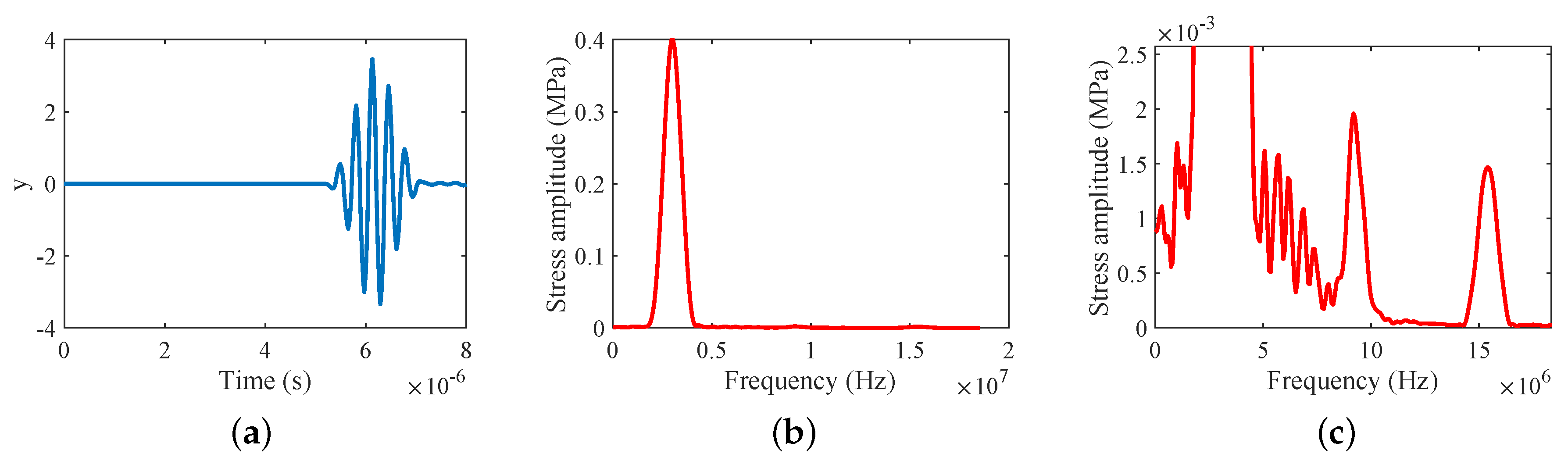
The resulting signal is shown in the Figure 16 when . It can be obviously seen that the third and fifth harmonics were generated by the second perturbation.
Current finite element simulation software requires that the deformation of mesh elements in simulation should not be too large or it can not guarantee the correctness of result. Therefore, the mesh elements should not be too small. On the other hand, if the objective is to measure the third or fifth harmonics, mesh elements must be small enough as described in Equation (24). There is a contradiction between the two theories, so there was no need to compare the amplitude of the third and fifth harmonics in wave propagation.
5. Conclusions
In this manuscript, three types of constitutive relations are reviewed and their subroutines with recursive expression are written. Two kinds of simulation models are established. One is to verify the correctness of subroutines, and the other is to conduct ultrasonic simulation. From the result of the verifying model, the subroutines of the first and second order perturbations satisfy the nonlinear theory. Hysteretic material simulation shows the deterioration process of materials, but it cannot be directly used to simulate the damaged materials and some analyses are made on it. Finally, the simulation of the first and second order perturbation shows that the harmonics appear. Especially, nonlinear coefficient increases with propagation distance in first order perturbation simulations and odd harmonics of the second order perturbation simulations are obvious. The work in this manuscript provides a new idea for the simulation of nonlinear ultrasonic testing.
There is still some follow-up work to be studied. Firstly, although recurrence equations can improve the calculation speed, it is not suitable to study the hysteresis material directly. Secondly, the current FE simulation software cannot guarantee the accuracy when the mesh element deformation is too large. Thirdly, the recurrence equations are not verified in three-dimensional simulation.
Author Contributions
Conceptualization, Z.Z., S.W. and F.W.; data curation, Z.Z.; formal analysis, Z.Z.; funding acquisition, F.W. and S.H.; investigation, Z.Z. and S.W.; methodology, Z.Z.; project administration, S.W. and F.W.; resources, Z.Z., S.W. and F.W.; supervision, S.W. and F.W.; validation, Z.Z.; writing—original draft, Z.Z.; writing—review and editing, Z.Z., S.W., F.W., S.H., W.Z. and Z.W. All authors have read and agreed to the published version of the manuscript.
Funding
This research was funded by National Key Research and Development Program grant number 2018YFC0809002.
Acknowledgments
The author greatly appreciates the help of translator Mengyuan Cui.
Conflicts of Interest
The authors declare no conflicts of interest.
References
- Farrar, C.R.; Worden, K. An introduction to structural health monitoring. Philos. Trans. A Math. Phys. Eng. Sci. 2007, 365, 303–315. [Google Scholar] [CrossRef] [PubMed]
- Marcantonio, V.; Monarca, D.; Colantoni, A.; Cecchini, M. Ultrasonic waves for materials evaluation in fatigue, thermal and corrosion damage: A review. Mech. Syst. Signal Process. 2019, 120, 32–42. [Google Scholar] [CrossRef]
- Blanloeuil, P.; Rose, L.; Veidt, M.; Wang, C.H. Time reversal invariance for a nonlinear scatterer exhibiting contact acoustic nonlinearity. J. Sound Vib. 2019, 417, 413–431. [Google Scholar] [CrossRef]
- Aleshin, V.; Delrue, S.; Trifonov, A.; Matar, O.B.; Abeele, K.V.D. Two dimensional modeling of elastic wave propagation in solids containing cracks with rough surfaces and friction—Part I: Theoretical background. Ultrasonics 2017, 82, 11–17. [Google Scholar] [CrossRef]
- Kim, J.; Park, S.J.; Yim, H. Nonlinear Resonance Vibration Assessment to Evaluate the Freezing and Thawing Resistance of Concrete. Materials 2019, 12, 325. [Google Scholar] [CrossRef] [Green Version]
- Meyendorf, N.G.; Rösner, H.; Kramb, V.; Sathish, S. Thermo-acoustic fatigue characterization. Ultrasonics 2002, 40, 427–434. [Google Scholar] [CrossRef]
- Cantrell, J.H. Substructural organization, dislocation plasticity and harmonic generation in cyclically stressed wavy slip metals. Proc. R. Soc. A Math. Phys. Eng. Sci. 2004, 460, 757–780. [Google Scholar] [CrossRef]
- Nagy, P.B. Fatigue damage assessment by nonlinear ultrasonic materials characterization. Ultrasonics 1998, 36, 375–381. [Google Scholar] [CrossRef]
- Herrmann, J.; Kim, J.Y.; Jacobs, L.J.; Qu, J.; Littles, J.W.; Savage, M.F. Assessment of material damage in a nickel-base superalloy using nonlinear Rayleigh surface waves. J. Appl. Phys. 2006, 99, 124913. [Google Scholar] [CrossRef]
- Kim, J.Y. Experimental characterization of fatigue damage in a nickel-base superalloy using nonlinear ultrasonic waves. J. Acoust. Soc. Am. 2006, 120, 1266–1273. [Google Scholar] [CrossRef]
- Raghavan, A. Guided-wave structural health monitoring. Diss. Abstr. Int. 2007, 975, 91–114. [Google Scholar] [CrossRef]
- Solodov, I.Y.; Krohn, N.; Busse, G. CAN: An example of nonclassical acoustic nonlinearity in solids. Ultrasonics 2002, 40, 621–625. [Google Scholar] [CrossRef]
- Zarembo, I.K.; Krasil’Nikov, V.A. Nonlinear Phenomena in the Propagation of Elastic Waves in Solids. Sov. Phys. Uspekhi 1970, 102, 778. [Google Scholar] [CrossRef] [Green Version]
- Jhang, K.Y.; Kim, K.C. Evaluation of material degradation using nonlinear acoustic effect. Ultrasonics 1999, 37, 39–44. [Google Scholar] [CrossRef]
- Zheng, Y.; Maev, R.G.; Solodov, I.Y. Nonlinear acoustic applications for material characterization: A review. Can. J. Phys. 1999, 77, 927–967. [Google Scholar] [CrossRef]
- Broda, D.; Staszewski, W.; Martowicz, A.; Uhl, T.; Silberschmidt, V. Modelling of nonlinear crack–wave interactions for damage detection based on ultrasound—A review. J. Sound Vib. 2014, 333, 1097–1118. [Google Scholar] [CrossRef]
- Hong, M.; Su, Z.; Wang, Q.; Cheng, L.; Qing, X. Modeling nonlinearities of ultrasonic waves for fatigue damage characterization: Theory, simulation, and experimental validation. Ultrasonics 2014, 54, 770–778. [Google Scholar] [CrossRef]
- Ruiz, A.; Ortiz, N.; Medina, A.; Kim, J.Y.; Jacobs, L. Application of ultrasonic methods for early detection of thermal damage in 2205 duplex stainless steel. NDT E Int. 2013, 54, 19–26. [Google Scholar] [CrossRef]
- Fierro, G.M.; Ciampa, F.; Ginzburg, D.; Onder, E.; Meo, M. Nonlinear ultrasound modelling and validation of fatigue damage. J. Sound Vib. 2015, 343, 121–130. [Google Scholar] [CrossRef] [Green Version]
- Ding, X.; Feilong, L.; Youxuan, Z.; Yongmei, X.; Ning, H.; Peng, C.; Mingxi, D. Generation Mechanism of Nonlinear Rayleigh Surface Waves for Randomly Distributed Surface Micro-Cracks. Materials 2019, 11, 644. [Google Scholar] [CrossRef] [Green Version]
- Wan, X.; Zhang, Q.; Xu, G.; Tse, P. Numerical Simulation of Nonlinear Lamb Waves Used in a Thin Plate for Detecting Buried Micro-Cracks. Sensors 2014, 14, 8528–8546. [Google Scholar] [CrossRef] [PubMed] [Green Version]
- Melchora, J.; Parnell, W.; Bochud, N.; Peralta, L.; Rusa, G. Damage prediction via nonlinear ultrasound: A micro-mechanical approach. Ultrasonics 2019, 93, 145–155. [Google Scholar] [CrossRef] [PubMed]
- Šofer, M.; Ferfecki, P.; Fusek, M.; Šofer, P.; Gnatowska, R.; Malujda, I.; Dudziak, M.; Krawiec, P.; Talaśka, K.; Wilczyński, D.A. The numerical analysis of the interaction between the low-order Lamb wave modes and surface breaking cracks. MATEC Web Conf. 2019, 254. [Google Scholar] [CrossRef]
- Cantrell, J.H.; Yost, W.T. Nonlinear ultrasonic characterization of fatigue microstructures. Int. J. Fatigue 2001, 23, 487–490. [Google Scholar] [CrossRef]
- Shui, G.; Wang, Y.; Qu, J. Advances in nodestructive test and evaluation of material degradation using nonlinear ultrasound. Adv. Mech. 2005, 35, 54–70. [Google Scholar]
- Jiao, J.; Lv, H.; He, C.; Wu, B. Fatigue crack evaluation using the non-collinear wave mixing technique. Smart Mater. Struct. 2017, 26, 65–71. [Google Scholar] [CrossRef]
- Landau, L.D.; Pitaevskii, L.P.; Kosevich, A.M.; Lifshitz, E.M. Theory of Elasticity; Elsevier Ltd.: Oxford, UK, 1986. [Google Scholar]
- Van Den Abeele, K.A.; Johnson, P.A.; Sutin, A. Nonlinear Elastic Wave Spectroscopy (NEWS) Techniques to Discern Material Damage, Part I: Nonlinear Wave Modulation Spectroscopy (NWMS). Res. Nondestruct. Eval. 2000, 12, 31–42. [Google Scholar] [CrossRef]
- Van Den Abeele, K.; Breazeale, M.A. Theoretical model to describe dispersive nonlinear properties of lead zirconate–titanate ceramics. J. Acoust. Soc. Am. 1996, 99, 1430–1437. [Google Scholar] [CrossRef]
- Jingpin, J.; Xiangji, M.; Cunfu, H.; Bin, W. Nonlinear Lamb wave-mixing technique for micro-crack detection in plates. NDT E Int. 2016, 85, 63–71. [Google Scholar] [CrossRef]
- Ostrovsky, L.A.; Johnson, P.A. Dynamic nonlinear elasticity in geomaterials. Riv. Nuovo Cimento della Soc. Ital. Fis. 2001, 24, 1–46. [Google Scholar]
Figure 1.
Schematic overview of the nonlinear contributions to the constitutive equation and its implication for dynamic one-dimensional wave propagation of a finite-amplitude monofrequency signal.
Figure 1.
Schematic overview of the nonlinear contributions to the constitutive equation and its implication for dynamic one-dimensional wave propagation of a finite-amplitude monofrequency signal.

Figure 2.
Geometry of the verifying model for simulations.

Figure 3.
Displacement signal for the right side boundary condition of the verifying model.

Figure 4.
The 2D wave propagation model and the place of excitation.

Figure 5.
(a) Temporal waveform of the excited tone burst signal. (b) Frequency spectrum of the excited tone burst signal.
Figure 5.
(a) Temporal waveform of the excited tone burst signal. (b) Frequency spectrum of the excited tone burst signal.

Figure 6.
Deformation of verifying model.

Figure 7.
Comparative analysis of strain and stress when is equal to 0 and −4,000,000 respectively.


Figure 8.
Stress-strain curves under different first order perturbations.
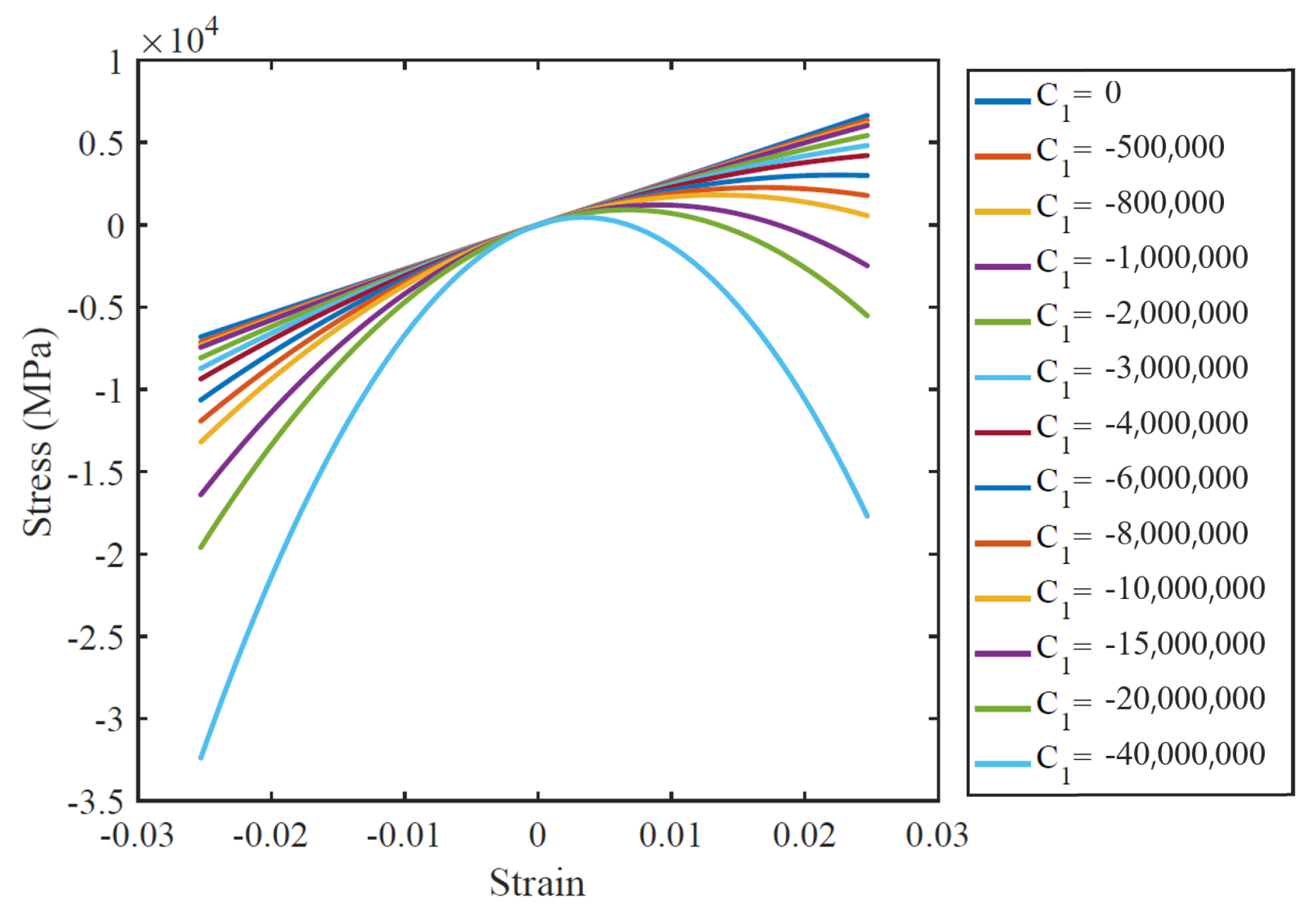
Figure 9.
Comparative analysis of strain and stress when is equal to 0 and respectively.
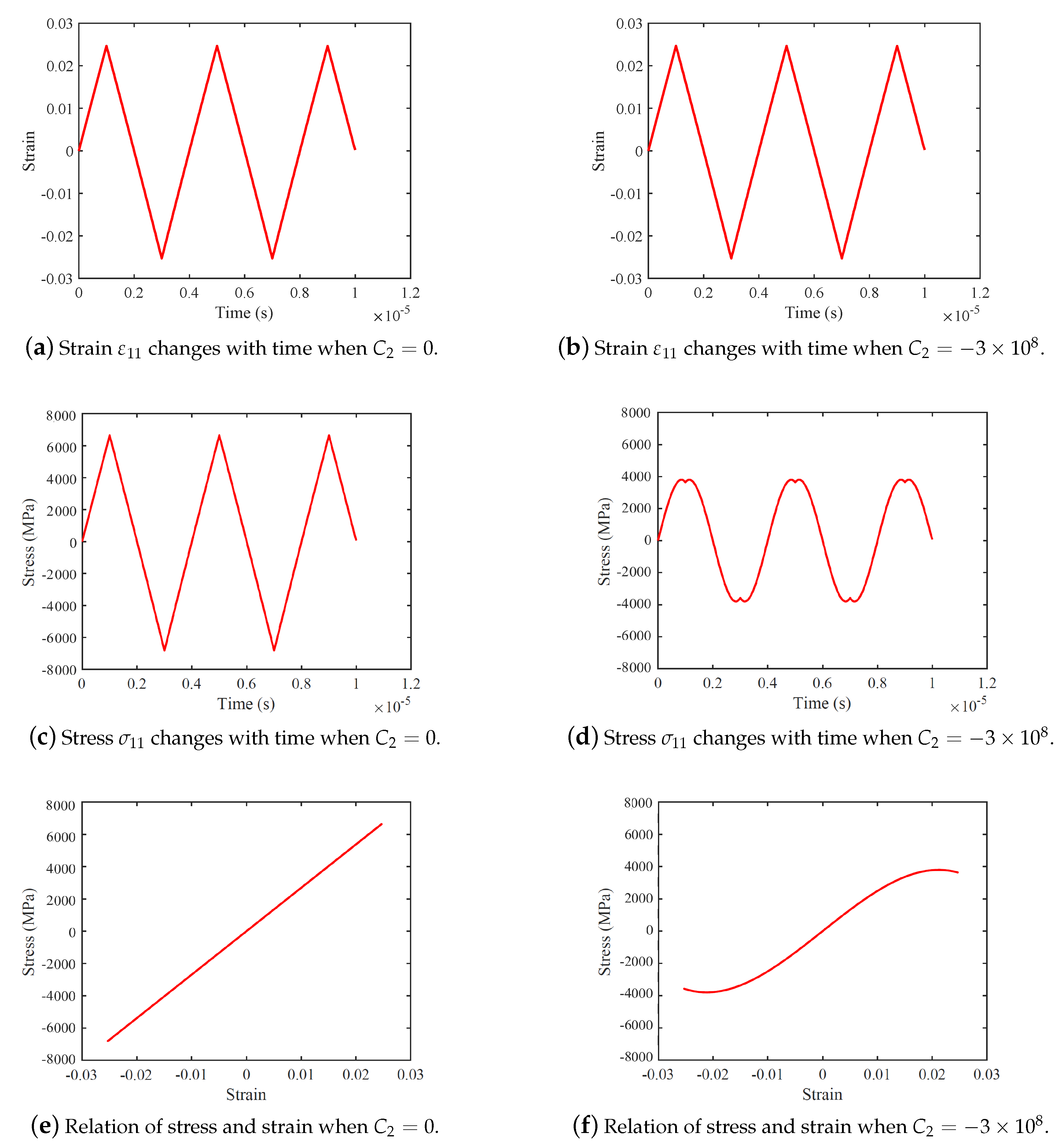
Figure 10.
Stress-strain curves under different second order perturbations.

Figure 11.
Simulation result of hysteretic material in the verifying model when .

Figure 12.
Stress-strain curves for different hysteresis.

Figure 13.
Stress nephogram at different times during ultrasonic propagation.


Figure 14.
Simulation result of the first order perturbation when 2,000,000: (a) Time domain signal. (b) Spectrum of signal. (c) Harmonic of signal.
Figure 14.
Simulation result of the first order perturbation when 2,000,000: (a) Time domain signal. (b) Spectrum of signal. (c) Harmonic of signal.
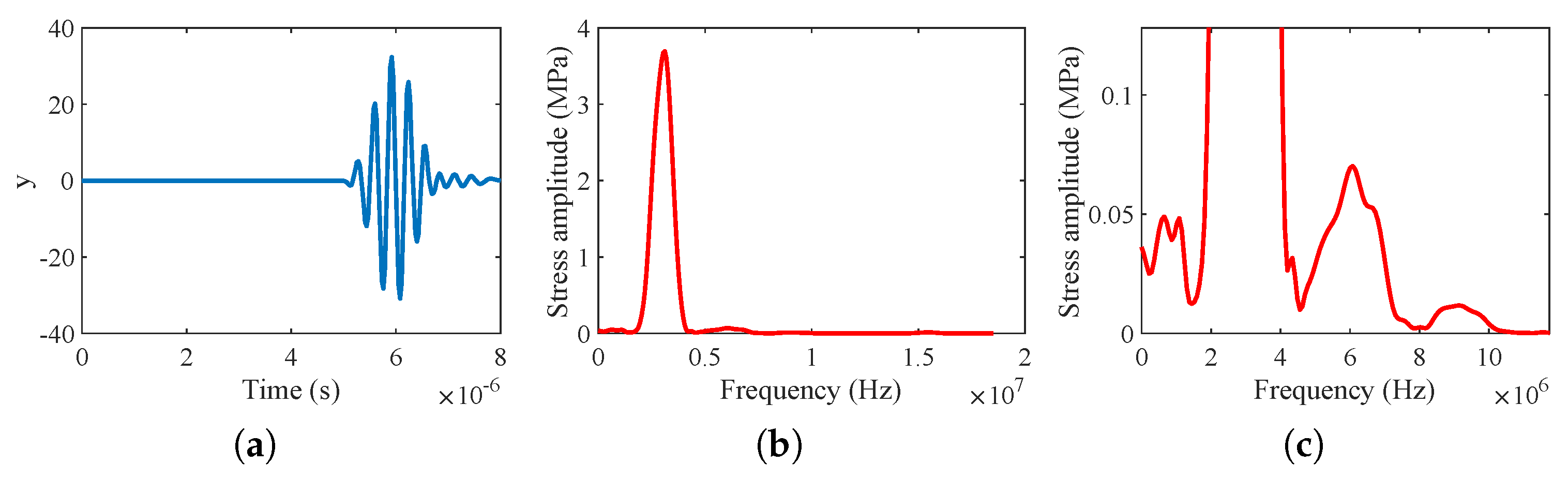
Figure 15.
Coefficient changes with propagation distance. (a) result of wave propagation model. (b) result from Ref [17].
Figure 15.
Coefficient changes with propagation distance. (a) result of wave propagation model. (b) result from Ref [17].

Figure 16.
Simulation result of second order perturbation when : (a) Time domain signal. (b) Spectrum of signal. (c) Harmonic of signal.
Figure 16.
Simulation result of second order perturbation when : (a) Time domain signal. (b) Spectrum of signal. (c) Harmonic of signal.

Table 1.
Main symbols used in the equation.
| Free energy | F |
| Lamé coefficients | , |
| Strain tensor | |
| Displacement component | |
| Cartesian coordinate | |
| Quadratic nonlinear perturbation coefficient | |
| Cubic nonlinear perturbation coefficient | |
| Hysteresis | |
| Simplified first perturbation coefficient | |
| Simplified second perturbation coefficient | |
| Simplified nonlinear hysteretic coefficient | |
| Young’s modulus | E |
| Kronecker symbol | |
| Strain rate |
Table 2.
Material properties in simulations.
| Material Type | Mass Density | Young’s Modulus | Poisson’s Ratio |
|---|---|---|---|
| Steel | 7800 kg/m | Pa | 0.3 |
© 2020 by the authors. Licensee MDPI, Basel, Switzerland. This article is an open access article distributed under the terms and conditions of the Creative Commons Attribution (CC BY) license (http://creativecommons.org/licenses/by/4.0/).
Share and Cite
MDPI and ACS Style
Zhan, Z.; Wang, S.; Wang, F.; Huang, S.; Zhao, W.; Wang, Z. Simulation of Three Constitutive Behaviors Based on Nonlinear Ultrasound. Appl. Sci. 2020, 10, 1982. https://doi.org/10.3390/app10061982
AMA Style
Zhan Z, Wang S, Wang F, Huang S, Zhao W, Wang Z. Simulation of Three Constitutive Behaviors Based on Nonlinear Ultrasound. Applied Sciences. 2020; 10(6):1982. https://doi.org/10.3390/app10061982
Chicago/Turabian StyleZhan, Zaifu, Shen Wang, Fuping Wang, Songling Huang, Wei Zhao, and Zhe Wang. 2020. "Simulation of Three Constitutive Behaviors Based on Nonlinear Ultrasound" Applied Sciences 10, no. 6: 1982. https://doi.org/10.3390/app10061982
Note that from the first issue of 2016, this journal uses article numbers instead of page numbers. See further details here.