Analysis of the Vibration Characteristics of Ballastless Track on Bridges Using an Energy Method


School of Civil Engineering, Beijing Jiaotong University, Beijing 100044, China
*
Author to whom correspondence should be addressed.
Appl. Sci. 2020, 10(7), 2289; https://doi.org/10.3390/app10072289
Submission received: 18 February 2020
/
Revised: 20 March 2020
/
Accepted: 23 March 2020
/
Published: 27 March 2020
(This article belongs to the Special Issue Interactions between Railway Subsystems)
Abstract
:Although the high-speed railway (HSR) system has been widely agreed to be a sustainable and convenient means of transportation, the vibration induced has already been deemed an urgent environmental problem. For the sake of investigating the vibration characteristics of the ballastless track on bridges in the HSR system from the point of view of energy, a numerical model of the vehicle–track–bridge coupled system is developed herein and the energy method based on power flow theory is employed. In addition, a corresponding evaluation method of the power flow theory is developed to evaluate the vibration characteristics of the track–bridge system. The conclusions indicate that (1) the vibration energy gradually attenuates from top to bottom of the track–bridge system in its transfer process. Moreover, the attenuation effects are mainly the result of the elasticity and damping effects of the fasteners and the slab mat layer. (2) With increasing slab mat layer stiffness, the vibration energy of the rail slightly decreases; on the contrary, that of the slab track and the bridge obviously increases. (3) With increasing fastener stiffness, the vibration energy of the entire track–bridge system increases. (4) With increasing running speed, the vibration energy of the entire track–bridge system rises obviously. The results reveal that the reasonable stiffness levels of the fasteners and the slab mat layer are 40 to 60 kN/mm and 40 to 60 MPa/m, respectively, under the investigated condition in this work. This work also presents a novel way to study the vibration characteristics of the ballastless track on bridges of HSRs in terms of energy.
1. Introduction
With the rapid development of the high-speed railway (HSR) system, the length of HSRs in service in China has exceeded 35,000 km, and the convenience brought has been obvious to all. However, the induced vibration and noise have become increasingly acute. Faced with these problems, numerous researchers have worked to address them. Liu et al. [1] proposed a vehicle–track coupled model in the frequency domain and utilized the compliance method to investigate the dynamic compliance for the vehicle–track system. Further, the structure-borne noises of a viaduct were analyzed via the finite element method (FEM). Jiang et al. [2] established a coupled model of the HSR simply supported beam bridge–track structure system (HSRBTS), in which the effect of shear deformation was taken into account. Moreover, the natural vibration characteristics of HSRBTS under different interlayer stiffness and lengths of rails at different subgrade sections were evaluated by means of the analytic method put forward in that paper. Wang et al. [3] carried out in situ testing on the environmental vibration response of the surrounding buildings and the ground caused by HSR trains, and the spectrum analysis method was used to study the vibration characteristics of the surrounding buildings and ground. Finally, the environmental vibration levels of HSRs were analyzed and evaluated. Toydemir et al. [4] used the FEM to determine the seismic performance levels of four bridges based on ambient vibration testing. For the vibration testing, they selected the Ankara–Sivas HSR line for analytical and experimental studies. To sum up, the vibration responses of the bridge were investigated by various methods.
Ballastless track systems have been widely adopted in the HSRs, such as the China Railways Track System (CRTS), and have the advantages of longer service life, lower cost of maintenance, better control of the track geometry, etc. For the ballastless track on bridges, laying a slab mat layer between the track and the bridge is an effective measure to reduce vibration. In all types of the CRTSs, the CRTS-II track, which consists of a track slab, CA (cement asphalt) mortar, base slab, and so on [5], has been widely employed in the HSR lines Beijing–Tianjin, Beijing–Shanghai, Beijing–Shijiazhuang, etc. Further, it has shown good performance overall.
For studying the vibration and noise induced by the HSRs, many scholars and researchers have focused on those induced in the CRTS-II track system. Li et al. [6] developed a coupled train–track–soil model, in which the multibody theory, FEM, and perfectly matched layers method were combined together to investigate the ground vibrations in HSR systems using the CRTS-II track. Wang et al. [7] established a frequency domain model to investigate the frequency response of the CRTS-II track. The vibrations of a vehicle–track coupled model of HSRs were studied. Liu et al. [8] developed a vehicle–track–subgrade coupled model based on the dynamic Biot’s equations to investigate the vibration responses of the coupled model, in which fluid–solid interaction was considered. Li et al. [9] established a vehicle–track–bridge–soil coupled model to analyze the influence of elastic bearings on ground vibrations when vehicles pass over the bridge. Wang et al. [10] established a vehicle–track–subgrade coupled model based on the vehicle–track coupling theory to investigate the effects of mortar debonding on the vibration properties of the CRTS-II track. The influences of different debonding lengths on the dynamic responses of the vehicle–track system were also researched by means of the FEM. Zhu and Cai [11] presented a 3D model based on the FEM to simulate interface damage between the track slab and CA mortar of the CRTS-II track, and they also established a vehicle–track coupled model to study the effects of interface damage of the slab track on vibrations.
At present, the methods of investigating the vibration of the track structure include field testing, FEM, numerical methods, etc. However, these methods are mainly focused on the instantaneous vibration responses in the time domain. Although many researchers and scholars have attached importance to the vibration responses in the frequency domain, the widely used indices, like the acceleration level, mobility, etc., are single evaluation indices. Further, the track–bridge system is a typical stratified structure from top to bottom, so its vibration mainly manifests as the transfer, storage, and consumption of energy in each component. To study the vibration characteristics of the track–bridge system, an energy method must be utilized. The energy method on the basis of power flow theory involves the amplitude and phase information of the force and velocity, which is not a single evaluation index. Its energy indices can be employed to evaluate the vibration damping performance. Goyder and White [12] and Pinnington and White [13] made contributions to the conceptual development of conducting power flow analysis of vibration isolation systems. Furthermore, research in many areas, like marine engineering, mechanical engineering, aerospace engineering, etc., has previously been conducted to study vibration characteristics based on this method. Therefore, the power flow method has potential applicability to investigating the vibration characteristics of the track–bridge system.
Bridges have been widely used in the HSR system because of their higher stability, but the induced vibration problem urgently needs to be solved. However, few researchers and scholars have carried out studies on the vibration energy of the ballastless track on bridges of the HSRs. Accordingly, the energy method based on power flow theory is applied in this work to study the vibration characteristics of the ballastless track on bridges of the HSRs. Further, a numerical model of the vehicle–track–bridge coupled system is established. The CRTS-II track, which has been widely employed in the HSR system in China, is taken into account. By means of the model, the effects of different track conditions and running speeds on the vibration energy are investigated.
2. Methods
In this section, the vehicle–track–bridge coupled system, which is composed of the vehicle model with two bogies, track–bridge model, and wheel/rail contact model, is established. The simulation results obtained by the system in the frequency domain are applied to conduct analysis of the power flows and corresponding evaluation indices.
2.1. Vehicle Model
This study takes the CRH3 vehicle (a vehicle which widely operates in the HSR system in China) as the modeling target, which is made up of one car body, two bogies, four wheelsets, suspension systems, etc. The vehicle model was developed according to multibody dynamic theory, and a rigid body with six degrees of freedom (DOF), which are in the vertical, lateral, longitudinal, pitching, yawing, and rolling directions, was employed to simulate the car body, bogies, and wheelsets. As a result, the elastic deformations of the components were ignored, and the total number of DOF was 42. Further, the suspension systems, which consist of the primary and secondary suspensions, were regarded as nonlinear springs connecting the car body, bogies, and wheelsets. This rigid vehicle model can be adopted to investigate the vibration of the vehicle–track–bridge system. However, due to neglect of the elastic deformation of the wheels, the rigid vehicle mode is deficient for investigating rail corrugation, wheel polygons, etc. A topological graph of the vehicle model is shown in Figure 1.
The dynamic formula of the vehicle motion is presented in Equation (1):
where Mv, Cv, and Kv denote the mass, damping, and stiffness matrices of the vehicle model; , and Zv refer to the acceleration, velocity, and displacement vectors; and Fv represents the force vector, which includes the external and internal force of the system. The parameters of the CRH3 vehicle are presented in Table 1.
2.2. Track–Bridge Model
The track–bridge model consists of the CRTS-II slab track and the simply supported beam bridge, as shown in Figure 2. The track structure includes the rails, fasteners, track slab, CA mortar, base slab, and slab mat layer. The bridge structure contains the bridge bodies and bridge piers, which are connected by bridge bearings. In order to depict the physical and geometric characteristics, except that the fasteners, the slab mat layer, and the bridge bearings were regarded as spring damper elements; the rest of the components in the track–bridge model were all simulated by solid elements, which can take deflection and shear deformation into account.
The kinematic equation of the track–bridge model is expressed by Equation (2):
where , and denote the mass, damping, and stiffness matrices of the track–bridge model, which are extracted and assembled by the mode superposition method; , and Zt refer to the acceleration, velocity, and displacement vectors of the track–bridge model; and Ft represents the load vector. The parameters of the track–bridge model are listed in Table 2.
2.3. Wheel/Rail Interaction Model
The vehicle and the track–bridge model are coupled by the interaction between the rails and wheels. In addition, the wheel/rail interaction model consists of two parts: (1) the solution of the wheel/rail contact geometry; (2) the solution of the wheel/rail contact force.
2.3.1. Wheel/Rail Contact Geometry
To solve the wheel/rail contact geometry, some assumptions need to be explained:
- (1)
- The wheels and rails are all considered rigid bodies.
- (2)
- The wheel/rail profiles are all discretized by means of cubic interpolation.
Based on those assumptions, the function of the wheel/rail relative displacement in the lateral direction can be employed to obtain the contact patch [14].
The contact geometry is illustrated in Figure 3. The coordinates of the wheel/rail contact point can be obtained by Equation (3):
where denotes the lateral distance between the rolling circle and the center of the wheelset axle; is the rolling radius of the wheel; represents the contact angle of the wheel tread; represents the lateral displacement of the wheelset; and . , , and refer to the cosine in the x, y, and z directions, which can be derived by Equation (4):
where and denote the rolling and yawing angles of the wheelset, respectively.
2.3.2. Wheel/Rail Contact Force
The solution of the wheel/rail contact force can be divided into two parts: a. the solution of the normal contact force; b. the solution of the tangent contact force.
(1) The Normal Contact Force
The solution of the normal contact force in this work is based on the theory presented by Hertz [15], which is not appropriate for solving the contact condition in turnouts or sharp curves. The mathematical expression is shown in Equation (5):
where is the elastic penetration at time t. G refers to the wheel/rail contact constant, which can be obtained by Equation (6):
where R represents the radius of the wheel.
The elastic penetration can be derived by the wheel/rail relative displacement, which is presented in Equation (7):
where Zwi(t) denotes the vertical displacement of wheels and Zri(t) refers to the vertical displacement of rails at the corresponding contact point.
(2) The Tangent Contact Force
Considering the occurrence of friction between the wheel and rail, tangent force is generated at the contact patch, namely, creep force. The solution of the tangent contact force is found on the basis of Kalker‘s linear theory [16], in which the distribution of the creep force is assumed to be symmetric, and Shen’s theory is employed to conduct nonlinear modification [17]. Based on the aforementioned two theories, the creep rates in the longitudinal, lateral, and spin directions are respectively defined in Equation (8):
where Vw1, Vw2, and Ωw3 denote the velocities of the wheel in the longitudinal, lateral, and spin directions, respectively; and Vr1, Vr2, and Ωr3 represent denote the velocities of the rail in the longitudinal, lateral, and spin directions, respectively.
The tangent contact force can be obtained by Equation (9):
where Tx and Ty refer to the creep forces in the longitudinal and lateral directions, respectively; Mz is the spin creep moment of force; E denotes the elastic modulus; a and b are the lengths of the semi-axes of the elliptical contact patch; and Cij represents Kalker’s coefficient, which can be obtained as a function of a/b and Poisson’s ratio.
2.4. Vibration Coupling Equation
The vibration coupling formula of the vehicle–track–bridge coupled system is presented in Equation (10):
where the notation is as defined before.
The motions of the vehicle–track–bridge coupled system are calculated and updated in each time step. Further, the vibration coupling equation is solved using the Newmark-β method.
2.5. Model Verification
To verify the validity of the model established in this paper, the simulated results in this work were compared with those by Chen et al. [18]. The simulation conditions are the same as those used by Chen et al. [18], including the vehicle speed of 360km/h, the track structure of the CRTS-II slab track on bridges, the vehicle type, etc. We consider that the critical indices in this work are the forces and velocities, and the acceleration can be converted into velocity by integration over time and is also the reflection of the forces. Therefore, we chose acceleration as the parameter for comparison. The comparisons of the dynamic responses are presented in Table 3. From Table 3, it can be observed that the simulation results of the numerical model developed in this work show little difference from those obtained by Chen et al. [18]. Accordingly, the model developed in this work can describe vibration responses of the track–bridge system accurately, and further simulations can be conducted using this model.
2.6. Description of Power Flow Theory
The average power flow method in the frequency domain was adopted in this paper to conduct analysis of the vibration energy. The mathematical expression [19] of the average power flow method is shown in Equation (11):
where F is the complex number value of forces in the frequency domain, that is, ; v denotes the complex number value of velocities in the frequency domain, that is, ; Re(.) represents the real part of a complex number; and superscript * refers to the complex conjugate.
To describe the influence of the impact effect on the vibration energy of the track–bridge system, the node power flows of the research area need to be summed up. The mathematical expression of the total power flow is presented in Equation (12):
where f denotes the calculated frequency and n is the number of nodes.
The power flow of the track–bridge system reflects the transfer of vibration energy in the components of the track–bridge system, and the vertical transfer of vibration energy is illustrated in Figure 4. In order to balance the accuracy and calculation cost and eliminate the influence of the boundary effect, a proper length of research area needs to be chosen. In this work, a length of track slab in the middle of the vehicle–track–bridge system was selected. Furthermore, the power flows of the rail and connecting elastic elements of the fasteners were regarded as the input vibration energy of the track–bridge system with the symbol Pin. The power flows of the slab track and connecting elastic elements of the slab mat layer were regarded as the input vibration energy of the slab track with the symbol P1. The power flows of the bridge body and the connecting elastic elements of the slab mat layer were then summed up as the input vibration energy of the bridge with the symbol P2. Finally, the power flow transfer from the bridge to the ground was denoted Pout.
After the total power flow of the track–bridge system is obtained, the relative power flow needs to be calculated for obvious comparisons. The mathematical expression is depicted in Equation (13):
where P(f) is the total power flow, which is determined by Equation (12); P0 denotes the reference power flow with a value of 1 × 10⁻⁸ N·m/s.
2.7. Evaluation Methodology
To evaluate the vibration energy of the track–bridge system, the average energy level of vibration (AELV) and the power flow transfer rate (PFTR) were proposed [20], which are the evaluation methodologies of the vibration energy and its vertical transfer, respectively.
The mathematical expression of the AELV is presented in Equation (14):
where F denotes the number of calculated frequency points.
The mathematical expression of the PFTR is presented in Equation (15):
where is the power flow of the lower component connected by the elastic elements, and refers to the power flow of the upper component connected by the elastic elements.
3. Results and Discussion
3.1. Vertical Transfer Characteristics of Vibration Energy
The running speed of the vehicle was set to 300km/h, and the power flows of the track–bridge system and corresponding evaluation indices were obtained under this condition. The frequency-domain velocity and force results of the rail and fasteners are shown in Figure 5 as an example.
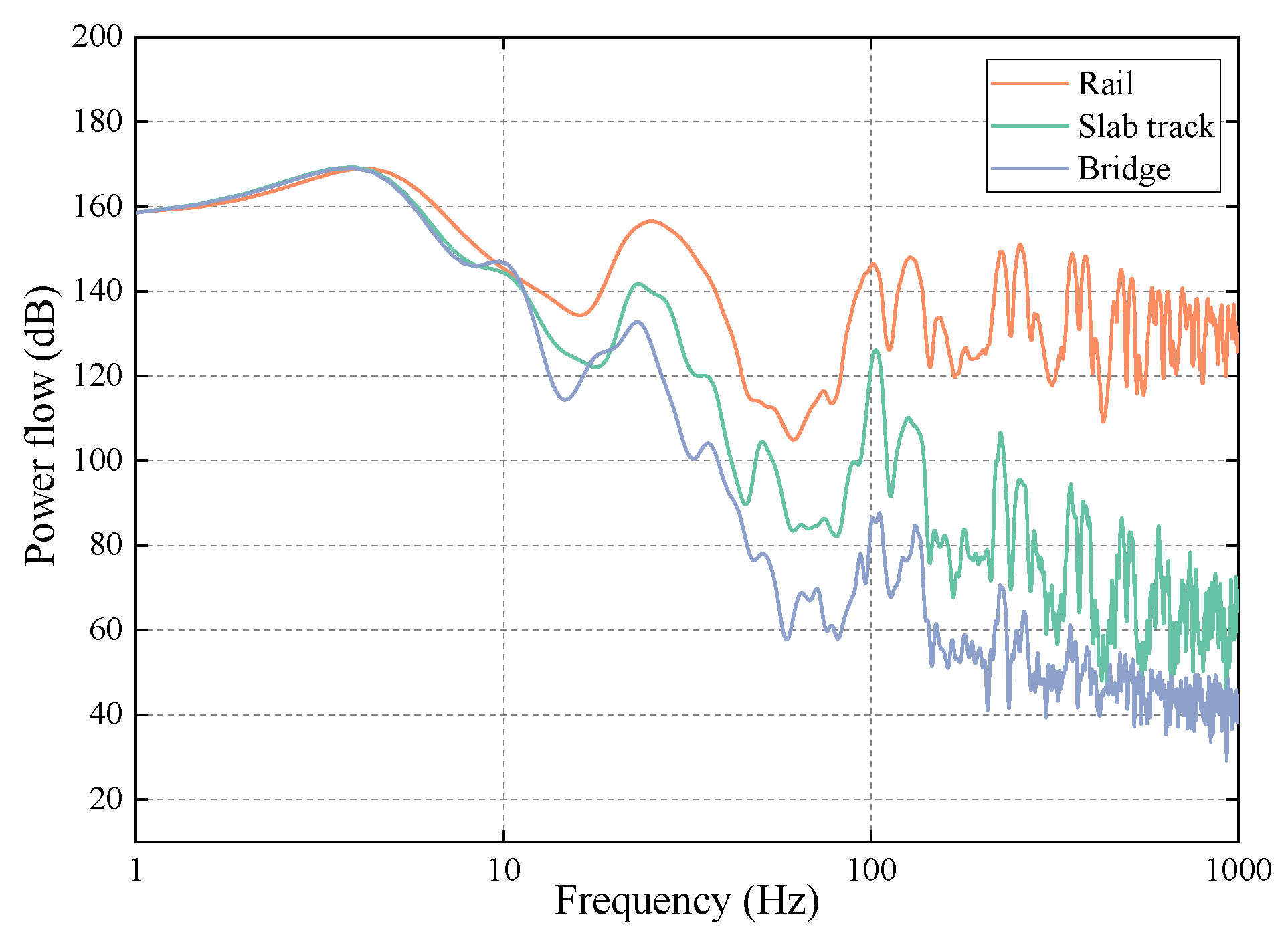
Figure 6 reveals that there were many peaks of power flows in the frequency range investigated. In addition, the power flows decreased obviously from top to bottom of the track–bridge system. This is because the vibration gradually attenuates from top to bottom of the track–bridge system in the transfer process. The differences in power flows between the rail and the slab track reflect the attenuation effect of the fasteners. In addition, the differences in power flows between the slab track and the bridge reflect the attenuation effect of the slab mat layer as well. Furthermore, the attenuation effect of fasteners is more significant in the frequency range of 150 Hz to 1000 Hz, that is, at a high frequency range, whereas the attenuation effect of the slab mat layer is more obvious in the frequency range of 45 Hz to 200 Hz, that is, at a low frequency range. Therefore, it can be inferred that the fasteners have an obvious damping effect at a high frequency range; on the contrary, the slab mat layer presents an evident damping effect at a low frequency range.
The PFTRs of the track–bridge system are shown in Figure 7. It can be observed that the PFTRs of the track–bridge system were all below 1.0, except for the power flows from the slab track to the bridge at some frequencies. In addition, the PFTRs from the rail to the slab track present a decreasing trend above 200 Hz, which is a result of the elasticity and damping effects of the fasteners. Nevertheless, the PFTRs from the slab track to the bridge show a downward trend in the frequency range of 10 Hz to 200 Hz, which is caused by the elasticity and damping effects of the slab mat layer. Therefore, conclusions can be drawn that the fasteners have a remarkable damping effect at a high frequency range, whereas the slab mat layer has a remarkable damping effect at a low frequency range.
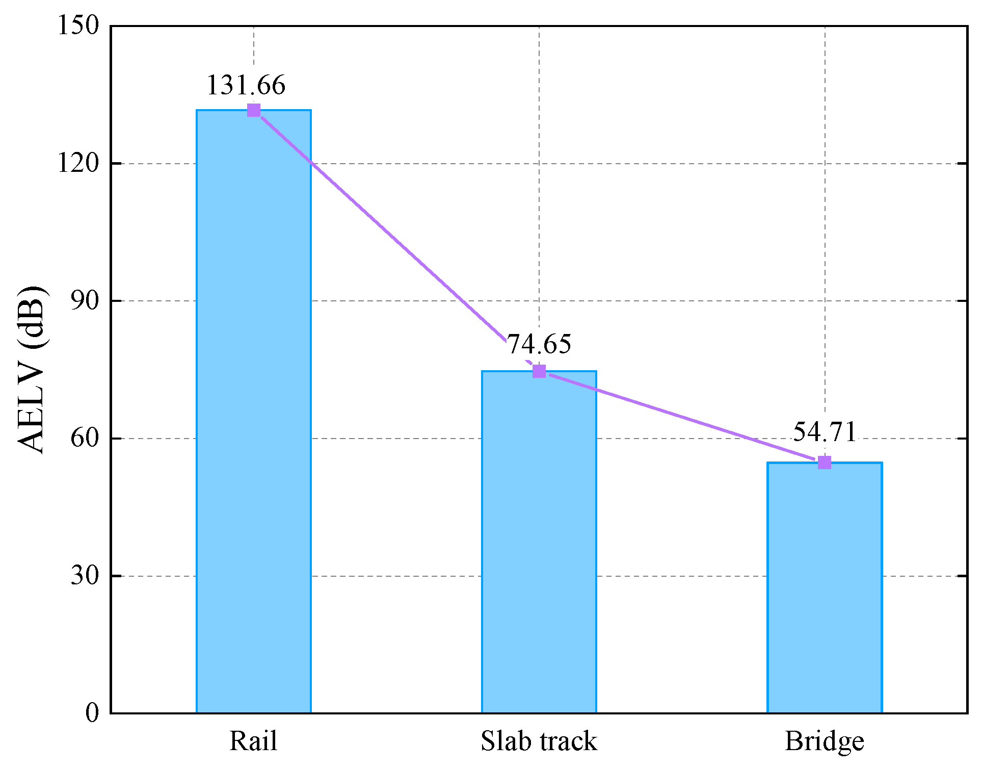
The AELVs of the track–bridge system are depicted in Figure 8. It can be observed that the AELVs of the rail, the slab, and the bridge present an order of large, medium, and small, respectively. This phenomenon arises from the elasticity and damping effects of fasteners and the slab mat layer. Moreover, the fasteners had a better vibration damping effect on the AELVs than the slab mat layer.
3.2. Influence of the Slab Mat Layer’s Stiffness
With the running speed of the vehicle set to the typical value of 300 km/h, conditions of the stiffness of the slab mat layer of 20 MPa/m, 40 MPa/m, 60 MPa/m, and 80 MPa/m were included. The influence of the slab mat layer’s stiffness on the vibration energy was thus investigated.
Figure 9 presents the influence of different stiffness levels of the slab mat layer on the power flows. It can be observed from Figure 9a that the changes in the slab mat layer’s stiffness mainly influenced the power flows of the rail below 80 Hz and scarcely affected the power flows above 80 Hz. In addition, the rail’s power flows decreased with increasing slab mat layer stiffness, except for at certain frequencies. Further, the changes from 20 MPa/m to 40 MPa/m are more obvious than those from 60 MPa/m to 80 MPa/m among the frequency ranges of 6 Hz to 28 Hz and 44 Hz to 66 Hz.
From Figure 9b, it can be observed that the variations in the slab track’s power flows were complicated with increasing slab mat layer stiffness. However, the slab track’s power flows for 20 MPa/m reached minima at frequencies of 60 Hz to 82 Hz and 161 Hz to 211 Hz, whereas they reached maxima at frequencies of 4 Hz to 9 Hz, 12 Hz to 28 Hz, and 37 Hz to 55 Hz. There were small differences in the power flows at other frequencies. From the above analysis, the influence of the stiffness of the slab mat layer on the power flows of the slab track mainly occurs below 80 Hz, that is, the low frequency range.
Figure 9c demonstrates that the bridge’s power flows for 80 MPa/m attained maxima at frequencies of 5 Hz to 12 Hz, 28 Hz to 48 Hz, 57 Hz to 150 Hz, and 217 Hz to 267 Hz. Further, the bridge’s power flows rose with increasing stiffness of the slab mat layer within the frequency ranges of 5 Hz to 12 Hz and 87 Hz to 139 Hz, and in those frequency ranges, greater stiffness of the slab mat layer was not in favor of reducing vibration. Besides this, differences in the stiffness of the slab mat layer had little effect on the power flows of the bridge above 270 Hz.
Figure 10 demonstrates the PFTRs of the track–bridge system with different stiffness levels of the slab mat layer. It can be observed from Figure 10a that the PFTRs were all below 1.0 when the vibration energy transferred from the rail to the slab track. In addition, the PFTRs for 20 MPa/m reached maxima at frequencies of 12 Hz to 30 Hz and 37 Hz to 46 Hz, whereas they reached minima at frequencies of 58 Hz to 92 Hz and 160 Hz to 212 Hz. There were few differences in the remaining frequency ranges.
Figure 10b shows that the PFTRs from the slab track to the bridge were all below 1.0, except for at some frequencies. Moreover, the PFTRs basically rose with increasing slab mat layer stiffness below 158 Hz; that is, the stiffness mainly plays a role in the PFTRs at a low frequency range. Therefore, if we employ greater stiffness of the slab mat layer in the low frequency range, more vibration energy will transfer to the bridge, which will go against the reduction of ambient vibration.
Figure 11 indicates the AELVs of the track–bridge system. It can be observed that although the variations of the AELVs of the rail were slight, the AELVs of the rail increased when the slab mat layer stiffness decreased. On the contrary, the changes in the AELVs of the slab track and the bridge are obvious, and the AELVs of the slab track and the bridge increased when the slab mat layer stiffness increased. Therefore, the AELVs of the slab tack and the bridge are more sensitive to changes in the slab mat layer’s stiffness than are those of the rail.
3.3. Influence of the Fasteners’ Stiffness
In this subsection, the power flows and corresponding indices are calculated for the running speed of 300 km/h when the fasteners’ stiffness is set to 20 kN/mm, 40 kN/mm, 60 kN/mm, and 80 kN/mm.
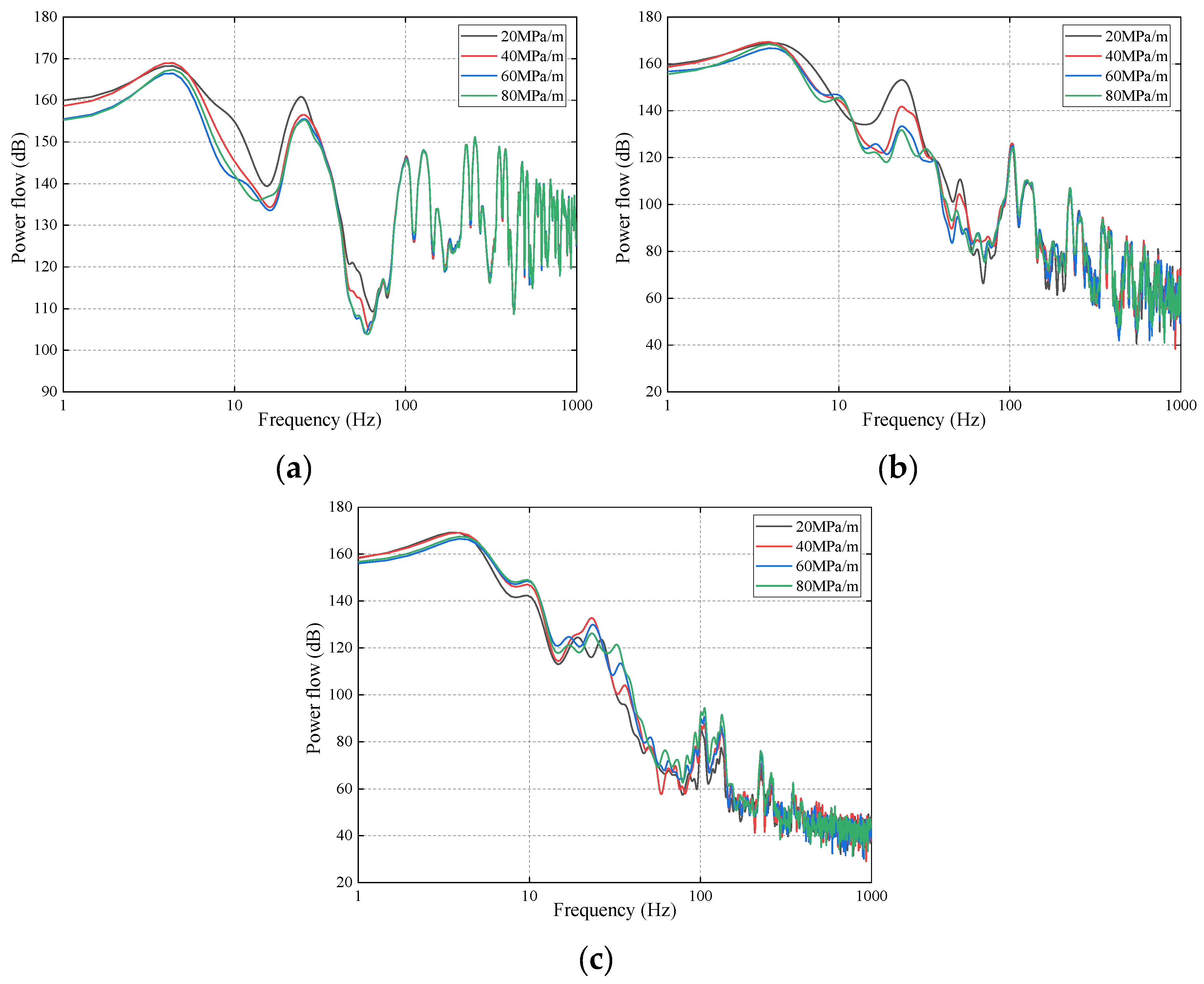
The power flows of the track–bridge system under different stiffness conditions are depicted in Figure 12. It can be observed from Figure 12a that the changes in the fasteners’ stiffness mainly had an effect on the power flows of the rail below 200 Hz, and there were little differences in the rail’s power flows above 200 Hz. In addition, the rail’s power flows decreased at frequencies below 200 Hz when the fasteners’ stiffness increased. Therefore, it can be said that variation in the fasteners’ stiffness mainly influences the power flows of the rail in a low frequency range. For the purpose of reducing rail vibration at the low frequency range, greater stiffness of the fasteners is recommended.
Figure 12b indicates that the slab track’s power flows increased when the fasteners’ stiffness rose at frequencies of 14 Hz to 67 Hz. The power flows of the slab track when applying fasteners of 20 kN/mm reached minima at frequencies of 1 Hz to 8 Hz as well. Although the power flows of the slab track showed little differences above 80 Hz, it can be inferred that the power flows with fastener stiffness of 80kN/mm were basically at maximum.
From Figure 12c, it can be observed that the bridge’s power flows did not simply vary when the fastener stiffness increased. The bridge’s power flows for 20 kN/mm reached minima at frequencies of 1 Hz to 7 Hz, 17 Hz to 30 Hz, and 63 Hz to 75 Hz. The bridge’s power flows for 40 kN/mm also reached minima at frequencies of 13 Hz to 17 Hz and 50 Hz to 62 Hz. Nevertheless, the bridge’s power flows when adopting the 80 kN/mm fasteners were mainly at maximum at the frequencies investigated.
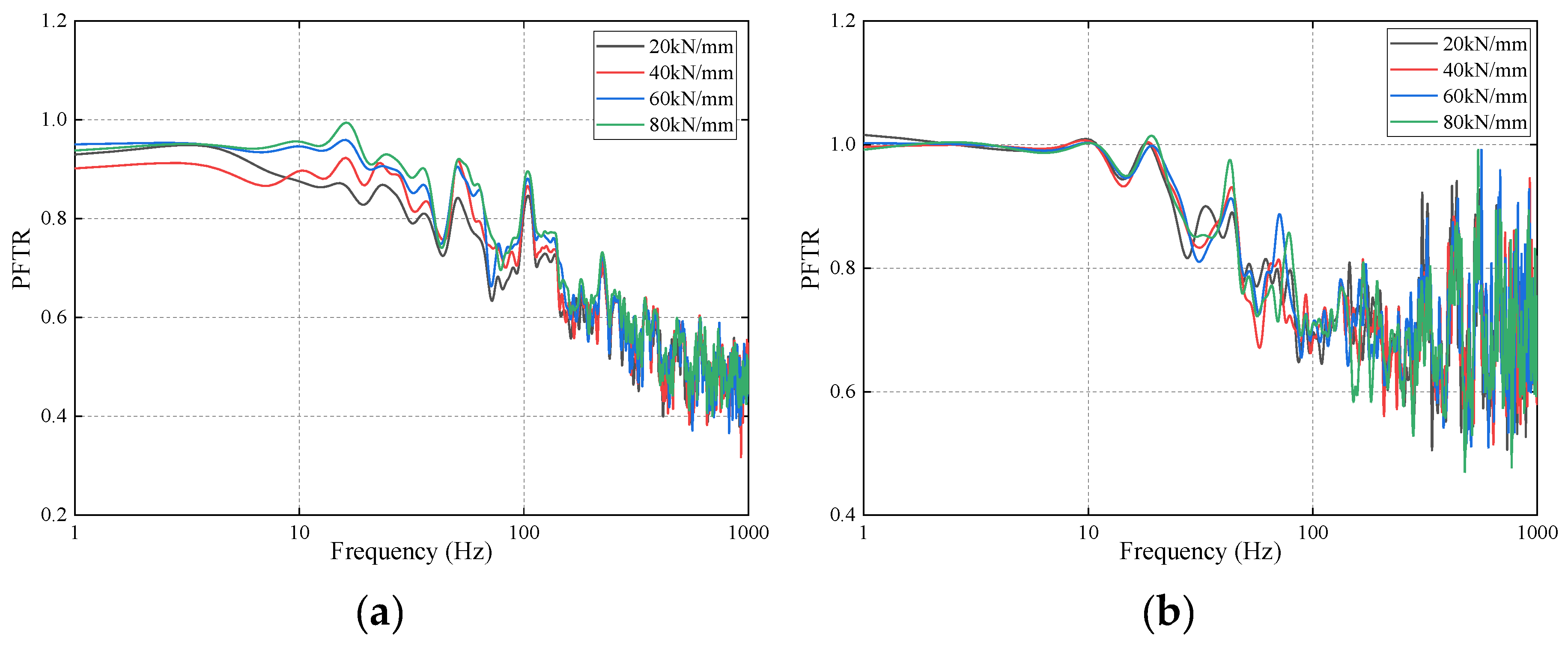
The PFTRs of the track–bridge system with different fastener stiffness levels are depicted in Figure 13. It can be seen from Figure 13a that the PFTRs were all below 1.0 when the vibration energy transferred from the rail to the slab track. Besides this, the PFTRs increased as the fasteners’ stiffness rose at frequencies of 9 Hz to 139 Hz, except for some frequencies. In addition, the PFTRs for 40kN/mm reached minima for frequencies below 9 Hz. The PFTRs for 80 kN/mm were basically at maximum in the frequency range investigated.
Figure 13b indicates that the PFTRs from the slab track to the bridge were around 1.0 when the frequencies were below 10 Hz and the PFTRs were smaller than 1.0, expect for some frequencies. The PFTRs of the bridge were maximum at the frequency of 19 Hz, reaching 1.015 with the stiffness of 80 kN/mm. The PFTRs under all four stiffness conditions presented little variation when the frequencies were larger than 190 Hz.
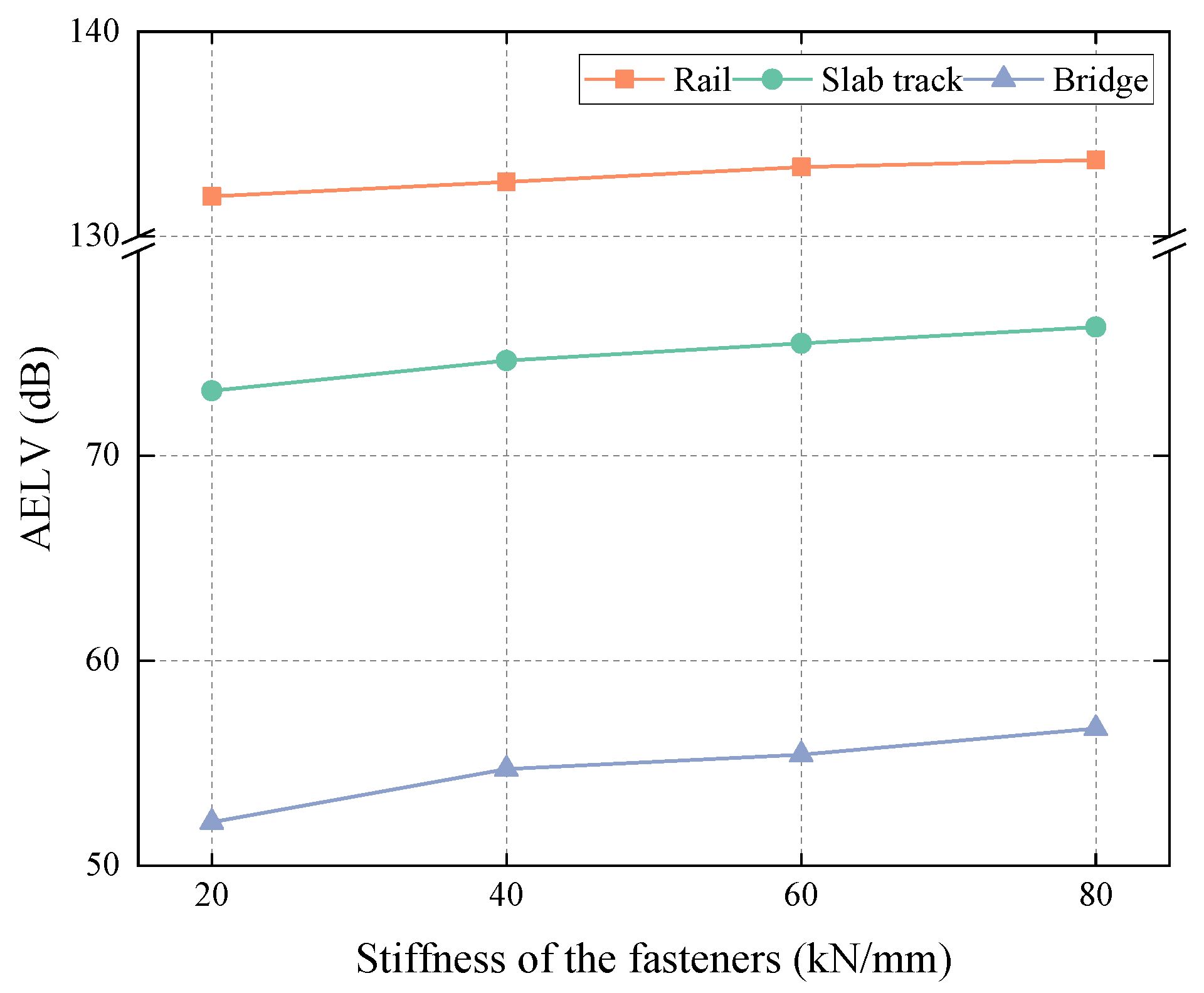
Figure 14 shows the AELVs of the track–bridge system. It can be clearly observed that the AELVs of the track–bridge system all increased as the fasteners’ stiffness rose. In other words, the track–bridge system stores more vibration energy when the fasteners’ stiffness increases. It can be concluded that the AELVs of the track–bridge system are sensitive to changes in the stiffness of the fasteners.
3.4. Influence of the Running Speed
The running speeds of 250 km/h, 300 km/h, and 350 km/h were selected to analyze their influence on the power flows and corresponding indices.
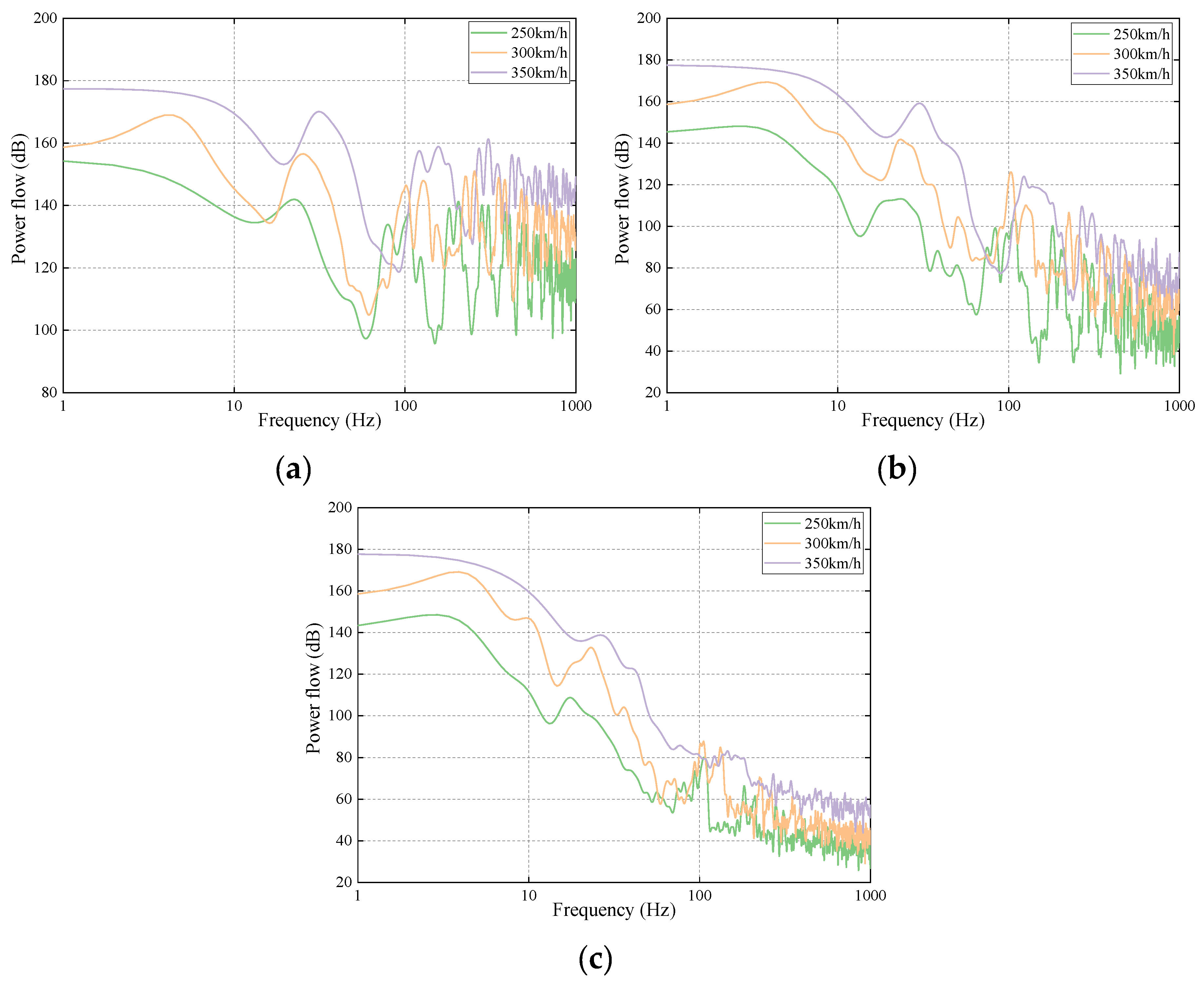
The power flows of the track–bridge system under different running speeds are depicted in Figure 15. It can be observed that there were phase differences in the power flows of the rail and the slab track, and the phase differences in the rail and the slab track were more obvious than those in the bridge. Considering these phase differences, it can be observed that the power flows of the track–bridge system rise as the running speeds increase, on the whole.
Figure 16 illustrates the track–bridge system’s PFTRs. It can be observed from Figure 16 that the PFTRs were all smaller than 1.0, except for those from the slab track to the bridge at certain frequencies. Further, the PFTRs rose obviously when the running speeds increased at low frequency range, on the whole. Although the differences under different running speeds were small at the high frequency range, it also can be seen that the PFTRs basically increased with increasing running speed. Therefore, it can be said that the PFTRs of the track–bridge system increase with rising running speeds, on the whole.
From Figure 17, it can be observed that the AELVs of the track–bridge system all increased with the growth of the running speed; that is, the higher the running speed, the more vibration energy the track–bridge system stored. The increments of the bridge were a little smaller than those of the rail and the slab track. Finally, it can be concluded that the AELVs of the track–bridge system are all sensitive to variation in the running speed.
4. Conclusions
In this paper we presented an energy method based on power flow theory to investigate the vibration characteristics of the ballastless track on bridges. Firstly, the methodology of the numerical model of the vehicle–track–bridge coupled system, power flow theory, and the corresponding evaluation methods were presented. Then, the vibration characteristics under different running speeds and various stiffness levels of the fasteners and slab mat layer were investigated. The major conclusions of this work are as below:
- (1)
- The vibration energy declined obviously from top to bottom of the track–bridge system at the frequencies investigated. This is because the energy gradually attenuates from top to bottom in the transfer process. Moreover, the attenuation effects are mainly the result of the elasticity and damping effects of the fasteners and the slab mat layer.
- (2)
- With increasing slab mat layer stiffness, the vibration energy of the rail decreased slightly; on the contrary, that of the slab track and the bridge increased obviously. That is to say, the vibration energy of the rail is less sensitive than that of the slab tack and the bridge to changes in the slab mat layer stiffness. Therefore, the stiffness of the slab mat layer employed ought to be a suitable value; a larger one would cause more environmental vibration, and a smaller one would cause rail defects, even polygonal wheels.
- (3)
- With increasing fastener stiffness, the vibration energy of the entire track–bridge system increased, as the track–bridge system stores more vibration energy under such conditions. It can be inferred that variation in the fasteners’ stiffness plays an important part in the vibration energy of the track–bridge system. To sum up, the stiffness of the fasteners employed ought to be a suitable value as well; larger stiffness would cause an increase in the ambient vibration, while smaller stiffness would affect the running safety of the vehicle.
- (4)
- With increasing running speed, the vibration energy of the track–bridge system increased obviously. That is to say, the running speed is a sensitive index for the vibration energy of the track–bridge system. Therefore, it can be concluded that the running speed plays an important part in the vibration energy of the track–bridge system as well.
The results reveal that reasonable stiffness levels of the fasteners and the slab mat layer are 40 to 60kN/mm and 40 to 60 MPa/m, respectively, under the conditions investigated in this work. Further, the findings in this work provide a novel way to investigate the vibration characteristics of track–bridge systems in terms of energy, and the developed model can be adopted to study the vibration characteristics of the ballastless track on bridges of HSRs once the corresponding parameters have been determined.
Author Contributions
Conceptualization, H.J. and L.G.; methodology, H.J. and L.G.; validation, H.J. and L.G.; formal analysis, H.J. and L.G.; investigation, H.J. and L.G.; data curation, H.J. and L.G.; writing—original draft preparation, H.J. and L.G.; writing—review and editing, H.J. and L.G.; visualization, H.J. and L.G.; funding acquisition, L.G. All authors have read and agreed to the published version of the manuscript.
Funding
This research was funded by the National Natural Science Foundation of China under Grant 51827813, and by the Key Program of National Natural Science Foundation of China under Grant U1734206.
Acknowledgments
The authors express their gratitude to the anonymous reviewers and Yinan Zhao for their valuable advice.
Conflicts of Interest
The authors declare no conflict of interest.
References
- Liu, L.; Song, R.; Zhou, Y.; Qin, J. Noise and Vibration Mitigation Performance of Damping Pad under CRTS-III Ballastless Track in High Speed Rail Viaduct. KSCE J. Civ. Eng. 2019, 23, 3525–3534. [Google Scholar] [CrossRef]
- Jiang, L.; Feng, Y.; Zhou, W.; He, B. Vibration characteristic analysis of high-speed railway simply supported beam bridge-track structure system. Steel Compos. Struct. 2019, 31, 591–600. [Google Scholar]
- Wang, X.; Zhang, H.; Xie, W. Field test and analysis of the environmental vibration characteristics of building nearby the high speed railway. J. Civ. Archit. Environ. Eng. 2018, 3, 16–22. [Google Scholar]
- Toydemir, B.; Kocak, A.; Sevim, B.; Zengin, B. Ambient vibration testing and seismic performance of precast I beam bridges on a high-speed railway line. Steel Compos. Struct. 2017, 23, 557–570. [Google Scholar] [CrossRef]
- Feng, Q.; Chao, H.; Lei, X. Influence of the Seam between Slab and CA Mortar of CRTSII Ballastless Track on Vibration Characteristics of Vehicle-Track System. Procedia Eng. 2017, 199, 2543–2548. [Google Scholar] [CrossRef]
- Li, T.; Su, Q.; Kaewunruen, S. Influences of piles on the ground vibration considering the train-track-soil dynamic interactions. Comput. Geotech. 2020, 120, 103455. [Google Scholar] [CrossRef]
- Wang, P.; Xu, J.; Wang, L.; Wei, K. Calculation model of the vehicle-CRTS II coupling system with symplectic method. Proc. Inst. Mech. Eng. Part F 2018, 232, 959–969. [Google Scholar] [CrossRef]
- Liu, K.; Yue, F.; Su, Q.; Liu, B.; Zhou, P. Investigation of Concrete Base-Roadbed Surface Contact Variation-Induced Vibration Characteristics of Vehicle-Slab Track-Subgrade System considering Fluid-Solid Interaction. Shock Vib. 2019, 2019, 1570736. [Google Scholar] [CrossRef]
- Li, X.; Zhang, Z.; Zhang, X. Using elastic bridge bearings to reduce train-induced ground vibrations: An experimental and numerical study. Soil Dyn. Earthq. Eng. 2016, 85, 78–90. [Google Scholar] [CrossRef]
- Wang, P.; Xu, H.; Chen, R. Effect of cement asphalt mortar debonding on dynamic properties of CRTS II slab ballastless track. Adv. Mater. Sci. Eng. 2014, 2014, 193128. [Google Scholar] [CrossRef] [Green Version]
- Zhu, S.; Cai, C. Interface damage and its effect on vibrations of slab track under temperature and vehicle dynamic loads. Int. J. Nonlin. Mech. 2014, 58, 222–232. [Google Scholar] [CrossRef]
- Goyder, H.G.D.; White, R.G. Vibrational power flow from machines into built-up structures. J. Sound Vib. 1980, 68, 59–117. [Google Scholar] [CrossRef]
- Pinnington, R.J.; White, R.G. Power flow through machine isolators to resonant and non-resonant beams. J. Sound Vib. 1981, 75, 179–197. [Google Scholar] [CrossRef]
- Kalker, J.J. The computation of three-dimensional rolling contact with dry friction. Int. J. Numer. Meth. Eng. 1979, 14, 1293–1307. [Google Scholar] [CrossRef]
- Hertz, H. Uber die beruhrung fester elastische korper und uber die harte (On the contact of rigid elastic solids and on hardness). Verhandlungen des Vereins zur Beforderung des Gewerbefleisses Leipzig 1882, 1882, 156–171. [Google Scholar]
- Kalker, J.J. A fast algorithm for the simplified theory of rolling contact. Veh. Syst. Dyn. 1982, 11, 1–13. [Google Scholar] [CrossRef]
- Shen, Z.Y.; Hedrick, J.K.; Elkins, J.A. A comparison of alternative creep force models for rail vehicle dynamic analysis. Veh. Syst. Dyn. 1983, 12, 79–83. [Google Scholar] [CrossRef]
- Chen, Z.; Zhai, W.; Yin, Q. Analysis of structural stresses of tracks and vehicle dynamic responses in train-track-bridge system with pier settlement. Proc. Inst. Mech. Eng. Part F 2018, 232, 421–434. [Google Scholar] [CrossRef]
- Li, W.L.; Lavrich, P. Prediction of power flows through machine vibration isolators. J. Sound Vib. 1999, 224, 757–774. [Google Scholar] [CrossRef]
- Jiang, H.; Gao, L. Study of the Vibration-Energy Properties of the CRTS-III Track Based on the Power Flow Method. Symmetry 2020, 12, 69. [Google Scholar] [CrossRef] [Green Version]
Figure 1.
A topological graph of the vehicle model.

Figure 2.
The track–bridge model.

Figure 3.
The contact geometry of the wheel/rail.
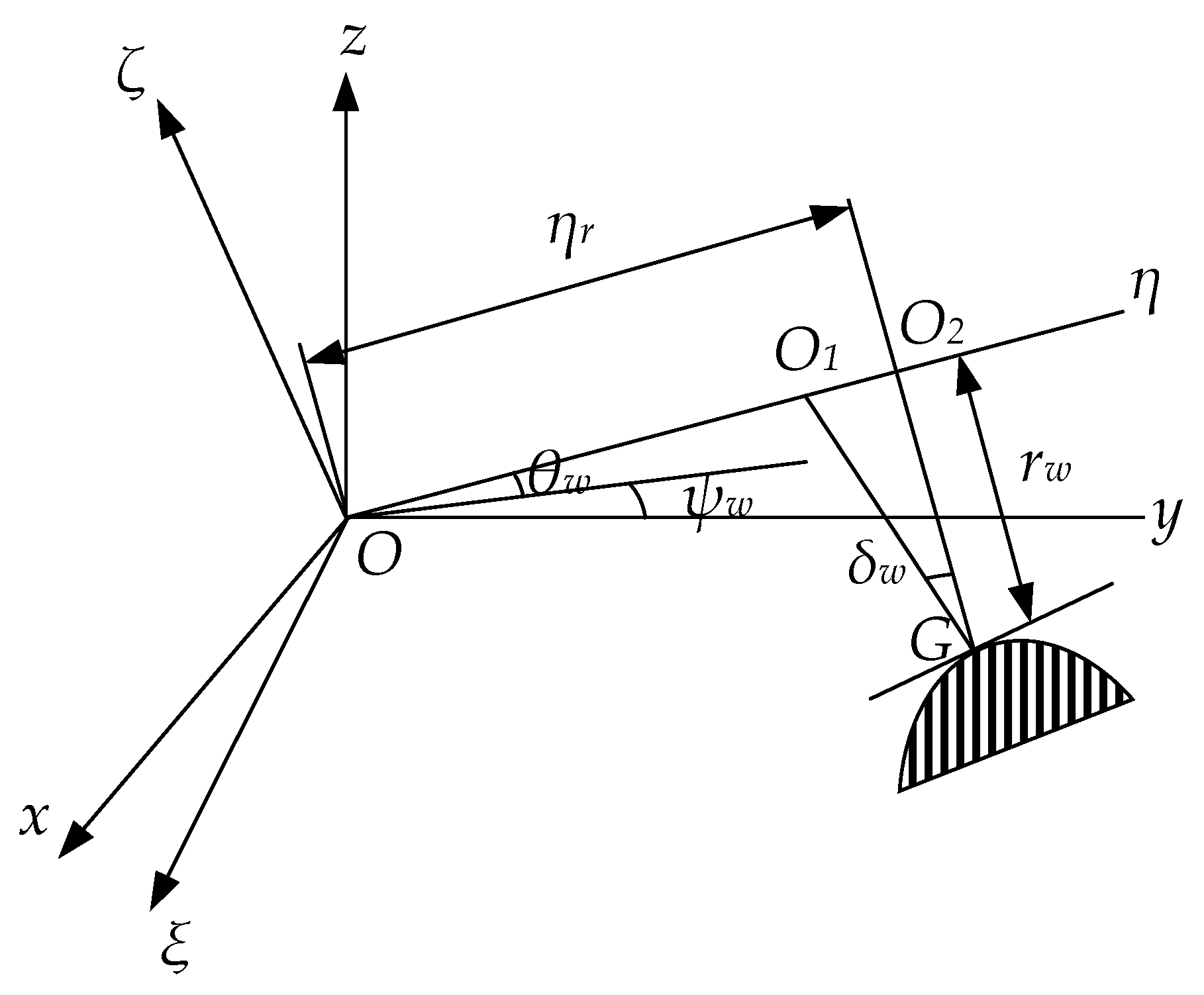
Figure 4.
The transfer of vibration energy.
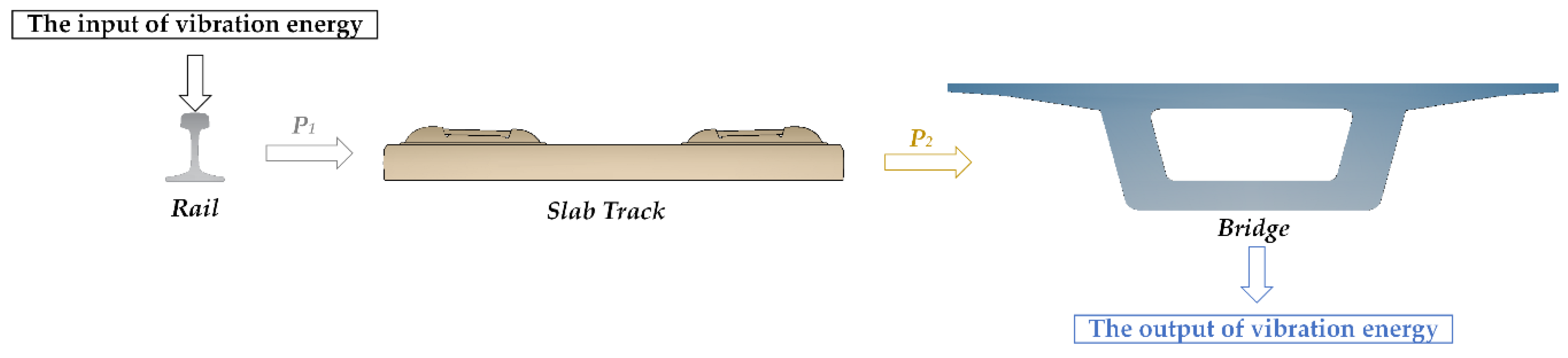
Figure 5.
The frequency-domain (a) velocity and (b) force results.
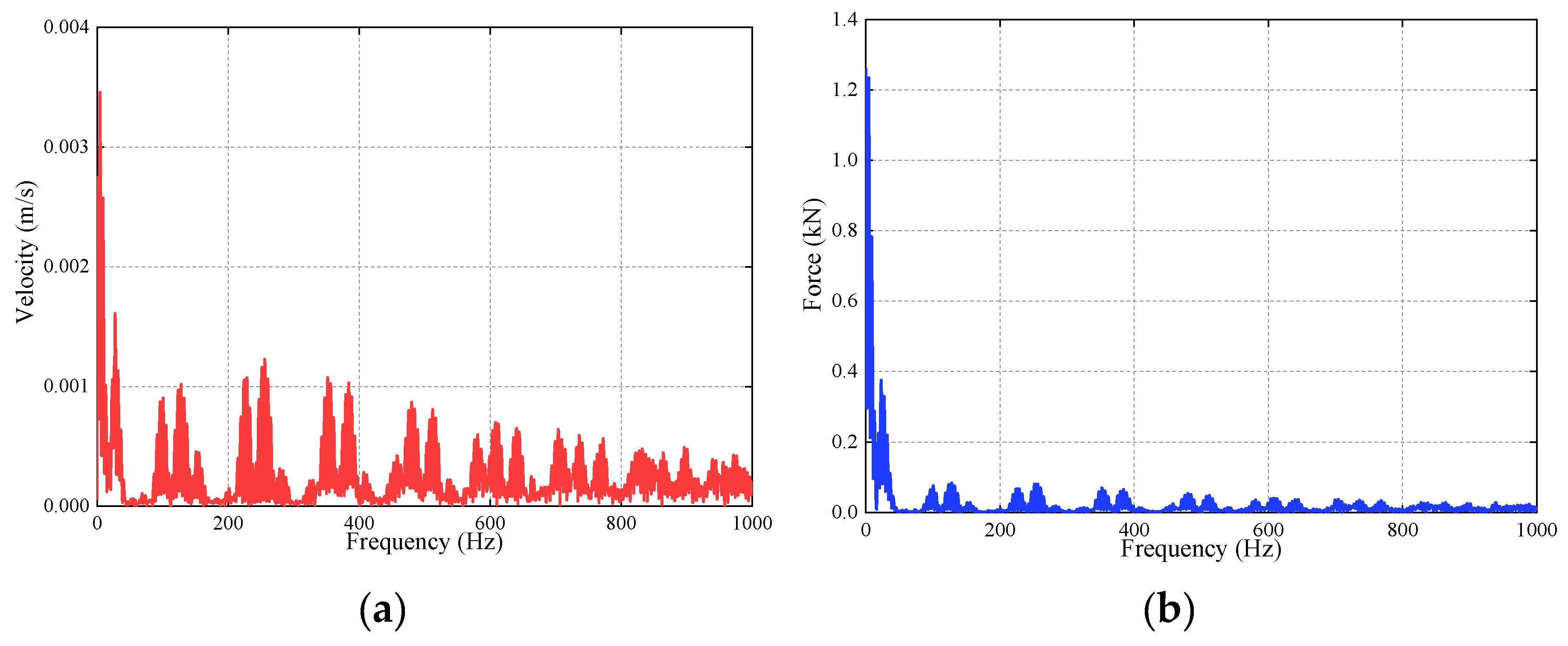
Figure 6.
The power flows of the track–bridge system.

Figure 7.
The power flow transfer rates (PFTRs) from (a) the rail to the slab track and (b) the slab track to the bridge.
Figure 7.
The power flow transfer rates (PFTRs) from (a) the rail to the slab track and (b) the slab track to the bridge.

Figure 8.
The average energy levels of vibration (AELVs) of the track–bridge system.

Figure 9.
The power flows of (a) the rail, (b) the slab track, and (c) the bridge.

Figure 10.
The PFTRs from (a) the rail to the slab track and (b) the slab track to the bridge.

Figure 11.
The AELVs of the track–bridge system.

Figure 12.
The power flows of (a) the rail, (b) the slab track, and (c) the bridge.

Figure 13.
The PFTRs from (a) the rail to the slab track and (b) the slab track to the bridge.

Figure 14.
The AELVs of the track–bridge system.

Figure 15.
The power flows of (a) the rail, (b) the slab track, and (c) the bridge.

Figure 16.
The PFTRs from (a) the rail to the slab track and (b) the slab track to the bridge.

Figure 17.
The AELVs of the track-bridge system.


Table 1.
The parameters of the CRH3 vehicle.
| Parameter | Unit | Value |
|---|---|---|
| Mass of car body/bogie/wheelset | kg | 40,200/2056/1627 |
| Car body pitching/yawing/rolling inertia | kg·m2 | 1.88 × 10⁶/1.85 × 106/1.06 × 105 |
| Bogie pitching/yawing/rolling inertia | kg·m2 | 7200/6800/3200 |
| Wheelset pitching/yawing/rolling inertia | kg·m2 | 120/1210/1210 |
| Lateral/vertical/longitudinal stiffness of primary suspension | MN/m | 3/1.04/9 |
| Lateral/vertical/longitudinal stiffness of secondary suspension | MN/m | 0.24/0.4/0.24 |
| Lateral/vertical/longitudinal damping of primary suspension | kN·s/m | 0/45/0 |
| Lateral/vertical/longitudinal damping of secondary suspension | kN·s/m | 30/50/500 |
| Radius of wheel | m | 0.46 |
| Distance between bogies | m | 17.375 |
| Distance between wheelsets | m | 2.5 |
Table 2.
The track–bridge model parameters.
| Parameter | Unit | Value |
|---|---|---|
| Mass of rail | kg/m | 60.64 |
| Cant of rail | 1:40 | |
| Elastic modulus of rail | GPa | 210 |
| Vertical/lateral stiffness of fasteners | kN/mm | 40/50 |
| Spacing distance of fasteners | m | 0.65 |
| Density of track slab | kg/m3 | 2500 |
| Elastic modulus of track slab | GPa | 35.5 |
| Density of CA mortar | kg/m3 | 2400 |
| Elastic modulus of CA mortar | GPa | 8.5 |
| Density of base slab | kg/m3 | 2500 |
| Elastic modulus of base slab | GPa | 30 |
| Surface stiffness of the slab mat layer | MPa/m | 40 |
| Length of track slab/CA mortar/bridge | m | 6.45/6.45/32 (× 4 span) |
| Density of bridge body | kg/m3 | 2600 |
| Elastic modulus of bridge body | GPa | 35.5 |
| Density of bridge pier | kg/m3 | 2500 |
| Elastic modulus of bridge pier | GPa | 30 |
Table 3.
Comparisons of the maximum dynamic responses.
| Dynamic Response | Rail vertical Acceleration (g) | Track Slab Vertical Acceleration (g) | Bridge Vertical Acceleration (g) |
|---|---|---|---|
| Chen et al. [18] | 139.2 | 3.6 | 0.24 |
| This paper | 136.8 | 3.5 | 0.21 |
© 2020 by the authors. Licensee MDPI, Basel, Switzerland. This article is an open access article distributed under the terms and conditions of the Creative Commons Attribution (CC BY) license (http://creativecommons.org/licenses/by/4.0/).
Share and Cite
MDPI and ACS Style
Jiang, H.; Gao, L. Analysis of the Vibration Characteristics of Ballastless Track on Bridges Using an Energy Method. Appl. Sci. 2020, 10, 2289. https://doi.org/10.3390/app10072289
AMA Style
Jiang H, Gao L. Analysis of the Vibration Characteristics of Ballastless Track on Bridges Using an Energy Method. Applied Sciences. 2020; 10(7):2289. https://doi.org/10.3390/app10072289
Chicago/Turabian StyleJiang, Hanwen, and Liang Gao. 2020. "Analysis of the Vibration Characteristics of Ballastless Track on Bridges Using an Energy Method" Applied Sciences 10, no. 7: 2289. https://doi.org/10.3390/app10072289
Note that from the first issue of 2016, this journal uses article numbers instead of page numbers. See further details here.