Managing Energy Plus Performance in Data Centers and Battery-Based Devices Using an Online Non-Clairvoyant Speed-Bounded Multiprocessor Scheduling

Abstract

An efficient scheduling reduces the time required to process the jobs, and energy management decreases the service cost as well as increases the lifetime of a battery. A balanced trade-off between the energy consumed and processing time gives an ideal objective for scheduling jobs in data centers and battery based devices. An online multiprocessor scheduling multiprocessor with bounded speed (MBS) is proposed in this paper. The objective of MBS is to minimize the importance-based flow time plus energy (IbFt+E), wherein the jobs arrive over time and the job’s sizes are known only at completion time. Every processor can execute at a different speed, to reduce the energy consumption. MBS is using the tradition power function and bounded speed model. The functioning of MBS is evaluated by utilizing potential function analysis against an offline adversary. For processors m ≥ 2, MBS is O(1)-competitive. The working of a set of jobs is simulated to compare MBS with the best known non-clairvoyant scheduling. The comparative analysis shows that the MBS outperforms other algorithms. The competitiveness of MBS is the least to date.

1. Introduction

There are number of server farms equipped with hundreds of processors. The cost of energy used for cooling and running a machine for around three years surpasses the hardware cost of the machine [1]. Consequently, the major integrated chips manufacturers such as Intel and AMD are producing the dynamic speed scaling (DSS) enabled multiprocessor/multi-core machine and software such as Intel’s SpeedStep [2], which support the operating system in managing the energy by varying the execution speed of processors. A founder chip maker Tilera forecasted that the numbers of processors/cores will be doubled every eighteen months [3], which will increase the energy demand to a great extent. Data centers consume 1.5% of total electricity usage in United States [4]. To avoid such critical circumstances, the current issue in the scheduling is to attain the good quality of service by generating an optimal schedule of jobs and to save the energy consumption, which is a conflicting and complicated problem [5].

The power P consumed by a processor running at speed s is $s{V}^2$, where V is a voltage [6]. The traditional power function is $P=s^{\alpha }$ ($\alpha \ge 2$ for CMOS based chips [7,8]). There are two types of speed models: the first unbounded speed model, in which the processor’s speed range is, i.e., $\left[0, \infty \right)$; the second bounded speed model, in which the speed of a processor can range from zero to some maximum speed, i.e., $\left[0, \eta \right]$. This DSS plays a vital role in energy management, where in a processor can regulate its speed to save energy. A few qualities of service metrics are slowdown, throughput, makespan, flow time and weighted flow time. At low speed, the processor finishes jobs slower and save energy, whereas at high speed, the processor finishes jobs faster but consumes more energy, as shown in Figure 1. To get a better quality of service and low energy consumption the objective should be to minimize the sum of flow time and energy; in case, if the importance or priority is attached, the objective should be to minimize the sum of importance-based flow time and energy. The objective of minimizing the IbFt+Ehas a natural explanation, as it can be considered in monetary terms [9].

In the multiprocessor systems, there is a requirement of three different policies: the first policy is job selection, which decides the next job to be executed on every processor; the second policy is speed scaling, which decides every processor’s execution speed at all time; the third policy is job assignment, which indicates that to which processor the new job should be assigned. In the c-competitive online scheduling algorithm, for each input the cost received is less than or equal to c times the cost of optimal offline algorithm [9]. Unlike non-clairvoyant scheduling, the size of job is unknown at arrival time, such as in UNIX operating system where jobs arrive with no information of processing requirement. Unlike online modes, in the offline mode, the whole job progression is known in advance. No online algorithm can attain a constant competitiveness with equal maximum speed to optimal offline algorithm [10].

Motwani et al. [10] commenced the study of the non-clairvoyant scheduling algorithms. Yao et al. inducted the theoretical study of speed scaling scheduling algorithm [11]. Yao et al. proposed an algorithm average rate heuristic (AVR) with a competitive ratio at most $2^{\alpha -1}{\alpha }^{\alpha }$ using the traditional power function. Koren et al. [12] presented an optimal online scheduling algorithm $D^{over}$ for a overloaded uniprocessor system with competitive ratio-$\left(\frac{1}{{\left(1+\sqrt{k}\right)}^2}\right)$ for the objective of minimizing the throughput, where k is the importance ratio. The competitiveness of shortest remaining processing time (SRPT) for multiprocessor system is $O\left(min\left(log\left(\raisebox{1ex}{$m$}\!\left/ \!\raisebox{-1ex}{$n$}\right.\right), log \sigma \right)\right)$, where m is number of processors, n is total number of jobs and $\sigma$ represents the ratio of minimum to maximum job size [13]. Kalyanasundaram et al. [14] presented the idea of resource augmentation. If the resources are augmented and, $\left(2+\Delta \right)$-speed p processors are used then the competitive ratio of Equi-partition lies between $\frac{2}{3}\left(1+\Delta \right)$ and $\left(2+\frac{4}{\Delta }\right)$ [15]. Multilevel feedback queue, a randomized algorithm with n jobs is $O\left(log n\right)$-competitive [16,17]. The first algorithm with non trivial guarantee is $O\left({\log }^2\sigma \right)$-competitive [18], where $\sigma$ is the ratio of minimum to maximum job size. There are different algorithms proposed with different objectives over a span of time [19,20,21,22,23,24,25,26,27].

Chen et al. [19] proposed algorithms with different approximation bounds for processors with/without constraints on the maximum processor speed. The concept of merging dual objective of energy used and total flow time into single objective of energy used plus total flow time is proposed by Albers et al. [20]. Bansal et al. [21] proposed an algorithm, which uses highest density first (HDF) for the job selection with a traditional power function. Lam et al. [22] proposed a multiprocessor algorithm for homogeneous processors in which job assignment policy is a variant of round robin, the job selection. Random dispatching can provide $\left(1+\Delta \right)$-speed $O\left(\raisebox{1ex}{$1$}\!\left/ \!\raisebox{-1ex}{${\Delta }^3$}\right.\right)$-competitive non-migratory algorithm [23]. Chan et al. [24] proposed an $O\left(1\right)$-competitive algorithm using sleep management for the objective of minimizing the flow time plus energy. Albers et al. [25] studied an offline problem in polynomial time and proposed a fully combitorial algorithm that relies on repeated maximum flow computation. Gupta et al. [26] proved that highest density first, weighted shortest elapsed time first and weighted late arrival processor sharing are not $O\left(1\right)$-speed $O\left(1\right)$-competitive for the objective of minimizing the weighted flow time even in fixed variable speed processors for heterogeneous multiprocessor setting. Chan et al. [27] studied an online clairvoyant sleep management algorithm scheduling with arrival-time-alignment (SATA) which is $\left(1+\Delta \right)$-speed $O\left(\raisebox{1ex}{$1$}\!\left/ \!\raisebox{-1ex}{${\Delta }^2$}\right.\right)$-competitive for the objective of minimizing the flow time plus energy. For a detailed survey refer to [28,29,30,31,32,33,34].

In this paper, the problem of online non-clairvoyant (ON-C) DSS scheduling is studied and an algorithm multiprocessor with bounded speed (MBS) is proposed with an objective to minimize the IbFt+E. On the basis of potential function analysis MBS is O(1)- competitive. The notations used in this paper are mentioned in the

Table 1. Notations used.

Notations	Meaning
t	Current time
j	A job
u	A processor
$r\left(j\right)$ or $r_j$	Release/arrival time of a job j
$p\left(j\right)$	Processing requirement (size) of a job j
$m$	Number of processors
$l{g}_u$	On a processor u, the count of lagging jobs, at time t
$\eta$	Maximum speed of a processor using Opt
P	Power of a processor at speed s
$s\left(t\right)$ or $s$	At time t, speed of some processor
$\alpha$	A constant, commonly believed that its value is 2 or 3
$\Delta$	A constant, its value depends on the value of $\alpha$
I, S	A set of jobs and their schedule, respectively
$pwk\left(j, t\right)$, $pw{k}_a\left(j, t\right)$ and $pw{k}_o\left(j, t\right)$	Remaining/pending work of a job j at time t, using MBS and Opt, respectively
$F\left(j\right)$	Flow time of a job j
F	Total importance-based flow time
$im{p}_{uj}\left(t\right)$ or $im{p}_u\left(j\right)$	Importance/weight of a job j, at time t on a processor u
$im{p}_{ua}\left(t\right)$ or $im{p}_{ua}$ and $im{p}_{uo}\left(t\right)$ or $im{p}_{uo}$	Importance of all active jobs using MBS and Opt at time t on a processor u, respectively
$im{p}_{lg}\left(t\right)$ or $im{p}_{lg}$ and $im{p}_{l{g}_u}\left(t\right)$ or $im{p}_{l{g}_u}$	Total importance of lagging jobs, at time t on all m processors and on a processor u, respectively
$n_a\left(t\right)$ or $n_a$ and $n_o\left(t\right)$ or $n_o$	Total number of active jobs (NoAJ) in MBS and Opt at time t on all m processors, respectively
$n_{ua}\left(t\right)$ or $n_{ua}$ and $n_{uo}\left(t\right)$ or $n_{uo}$	NoAJ in MBS and Opt at time t on a processor u, respectively
$s_{ua}\left(t\right)$ or $s_{ua}$ and $s_{uo}\left(t\right)$ or $s_{uo}$	Speed of a processor u for MBS and Opt at time t, respectively
$imp\left(t\right)$	Total importance of all active jobs $n_a$, at time t
$E$	Energy consumed by processors
G	Total IbFt+E
$c$	Competitiveness
$\mu$	A constant ($0<\mu <1$), its value depends on the value of $\Delta$
$G_a\left(t\right)$ or $G_a$ and $G_o\left(t\right)$ or $G_o$	IbFt+E acquired till time t by the MBS and Opt, respectively
$\frac{d{G}_a\left(t\right)}{dt}$ or $\frac{d{G}_a}{dt}$ and $\frac{d{G}_o\left(t\right)}{dt}$ or $\frac{d{G}_o}{dt}$	Rate of change (RoC) of $G_a$ due to MBS and $G_o$ due to Opt at time t, respectively
$G_{ua}\left(t\right)$ or $G_{ua}$ and $G_{uo}\left(t\right)$ or $G_{uo}$	IbFt+E acquired on a processor u till time t by the MBS and Opt, respectively
$\frac{d{G}_{ua}\left(t\right)}{dt}$ or $\frac{d{G}_{ua}}{dt}$ and $\frac{d{G}_{uo}\left(t\right)}{dt}$ or $\frac{d{G}_{uo}}{dt}$	RoC of $G_a$ due to MBS and Opt at time t on a processor u, respectively
$\gamma$	A constant (> 0)
$c_i$	Coefficient of a job $j_i$ at time t
${\omega }_i$	Difference of pending work of a job $j_i$ using MBS and Opt at time t
$\delta$	A constant depends on $\alpha$, its value is $\left(\frac{1}{2\alpha }\right)$
$L{G}_u$	A set of lagging jobs using MBS on a processor u
$LG$	A set of all lagging jobs using MBS on all m processors
$\Phi \left(t\right)$ or $\Phi$	Total potential value of all m processors at time t
${\Phi }_u\left(t\right)$ or ${\Phi }_u$	Potential value of a processor u at time t
$\frac{d{\Phi }_o}{dt}$ and $\frac{d{\Phi }_a}{dt}$	RoC of $\Phi$ due to Opt and MBS, respectively
$\frac{d\Phi }{dt}$	RoC of $\Phi$ due to Opt and MBS
$\frac{d{\Phi }_{uo}}{dt}$ and $\frac{d{\Phi }_{ua}}{dt}$	RoC of $\Phi$ due to Opt and MBS on a processor u, respectively
$\frac{d{\Phi }_u}{dt}$	RoC of $\Phi$ due to Opt and MBS on a processor u

.

The organization of the paper is as follows. In Section 2, some related non-clairvoyant algorithms are explained and their competitive values are compared to the proposed algorithm MBS. Section 3 presents the preliminary definition and information for the proposed work. In Section 4, the proposed algorithm, its flow chart and potential function analysis is presented. The processing of a set of jobs are simulated using MBS and the best identified algorithm to observe the working of MBS. Section 6 provides the conclusion and future scope of the work.

2. Related Work

Gupta et al. [35] gave an online clairvoyant scheduling algorithm GKP (proposed by Gupta, Krishnaswamy and Pruhs) for the objective of minimizing the weighted flow time plus energy. Under the traditional power function, GKP is $O\left({\alpha }^2\right)$-competitive without a resource augmentation for power heterogeneous processors. GKP uses highest density first (HDF) for the selection of jobs on each processor; the speed of any processor scales such that the power of a processor is the fractional weight of unfinished jobs; jobs are assigned in such a way that it gives the least increase in the projected future weighted flow time. Gupta et al. [35] used a local competitiveness analysis to prove their work. Fox et al. [36] considered the problem of scheduling the parallelizable jobs in the non-clairvoyant speed scaling settings for the objective of minimizing the weighted flow time plus energy and they used the potential function analysis to prove it. Fox et al. presented weighted latest arrival processor sharing with energy (WLAPS+E), which schedules the late arrival jobs and every job use the same number of machines proportioned by the job weight. WLAPS+E spares some machines to save the energy. WLAPS+E is $\left(1+6\Delta \right)$-speed $\left(\raisebox{1ex}{$5$}\!\left/ \!\raisebox{-1ex}{${\Delta }^2$}\right.\right)$-competitive, where $0<\Delta \le \raisebox{1ex}{$1$}\!\left/ \!\raisebox{-1ex}{$6$}\right.$. Thang [37] studied the online clairvoyant scheduling problem for the objective of minimizing the weighted flow time plus energy in the unbounded speed model and using the traditional power function. Thang gave an algorithm (ALG_Thang) on unrelated machines and proved that ALG_Thang is $8\left(1+\raisebox{1ex}{$\alpha $}\!\left/ \!\raisebox{-1ex}{$ln\alpha $}\right.\right)$-competitive. In AlG_Thang, the speed of any processor depends on the total weight of pending jobs on that machine, and any new job is assigned to a processor that minimizes the total weighted flow time.

Im et al. [38] proposed an ON-C scheduling algorithm SelfishMigrate-Energy (SM-E) for the objective of minimizing the weighted flow time plus energy for the unrelated machines. Using the traditional power function SM-E is $O\left({\alpha }^2\right)$-competitive. In SM-E, a virtual queue is maintained on every processor where the new or migrated jobs are added at tail; the jobs migrate selfishly until equilibrium is gained. Im et al. simulates sequential best response (SBR) dynamics and they migrates each job to the machine that is provided by the Nash equilibrium. The scheduling policy applied on every processor is a variant of weighted round robin (WRR), wherein the larger speed is allotted to jobs residing at the tail of the queue (like Latest Arrival Processor Sharing (LAPS) and Weighted Latest Arrival Processor Sharing (WLAPS)). Bell et al. [39] proposed an online deterministic clairvoyant algorithm dual-classified round robin (DCRR) for the multiprocessor system using the traditional power function. The motive of $\left(2^{4\alpha }\left(lo{g}^{\alpha }P+{\alpha }^{\alpha }{2}^{\alpha -1}\right)\right)$-competitive DCRR is to schedule the jobs so that they can be completed within deadlines using minimum energy, i.e., the objective is to maximize the throughput and energy consumption. In DCRR, the sizes and the maximum densities (= size/(deadline – release time)) of jobs are known and the classification of jobs depends on the size and the maximum density both. The competitive ratio of DCRR is high, as it considers the jobs with deadlines and using a variation of round robin with the speed scaling.

Azar et al. [40] gave an ON-C scheduling algorithm NC-PAR (Non-Clairvoyant for Parallel Machine) for the identical parallel machines, wherein the job migration is not permitted. Using traditional function NC-PAR is $\left(\alpha +\frac{1}{\alpha -1}\right)$-competitive for the objective of minimizing the weighted flow time plus energy in unbounded speed model. In NC-PAR a global queue of unassigned jobs is maintained in First In First Out (FIFO) order. A new job is assigned to a machine, when a machine becomes free. In NC-PAR jobs are having uniform density (i.e., $weight/size=1$) and the jobs are not immediately allotted to the processors at release time. The speed of a processor using NC-PAR is based on the total remaining weight of the active jobs. In non-clairvoyant model with known arbitrary weights no results are known [40].

An ON-C multiprocessor speed scaling scheduling algorithm MBS is proposed and studied against an offline adversary with an objective of minimizing IbFt+E. The speed of a processor using MBS is proportional to the sum of importance of all active jobs on that processor. In MBS, the processor’s maximum speed can be $\left(1+\raisebox{1ex}{$\Delta $}\!\left/ \!\raisebox{-1ex}{$3m$}\right.\right)\eta$ (i.e., the range of speed is from zero to $\left(1+\raisebox{1ex}{$\Delta $}\!\left/ \!\raisebox{-1ex}{$3m$}\right.\right)\eta$), whereas the processor’s maximum speed using Opt (Optimal algorithm) is $\eta$, where m is number of processors and $0<\Delta \le {\left(3\alpha \right)}^{-1}$ a constant. In MBS, a new job is assigned to an idle processor (if available) or to a processor having the minimum sum of the ratio of importance and executed size for all jobs on that processor; the policy for job selection is weighted/importance-based round robin, and each active job receives the processor speed equal to the ratio of its importance to the total importance of jobs on that processor. In this paper, the performance of MBS is analysed using a competitive analysis, i.e., the worst-case comparison of MBS and optimal offline scheduling algorithm. MBS is $\left(1+\raisebox{1ex}{$\Delta $}\!\left/ \!\raisebox{-1ex}{$3m$}\right.\right)$-speed, $\left(\frac{9}{8}+\frac{3\Delta }{8}\right)·\left(1+{\left(1+\raisebox{1ex}{$\Delta $}\!\left/ \!\raisebox{-1ex}{$3m$}\right.\right)}^{\alpha }\right)=O\left(1\right)$ competitive, i.e., the value for competitive ratio c for $m=2$, $\alpha =2$ is 2.442; for $m=2$, $\alpha =3$ is 2.399; the detailed results for different values of m, $\Delta ={\left(3\alpha \right)}^{-1}$ and $\alpha =2 \& 3$ is shown in

Table 2. Results of multiprocessor with bounded speed (MBS).

Number of Processors (m)	$\mathit{\alpha }=2$		$\mathit{\alpha }=3$
	Speed Ratio $\left({\mathit{s}}_{\mathit{r}}\right)$	Competitive Ratio (c)	Speed Ratio $\left({\mathit{s}}_{\mathit{r}}\right)$	Competitive Ratio (c)
2	1.02778	2.44189	1.01852	2.39936
4	1.01389	2.40822	1.00926	2.36604
8	1.00694	2.39155	1.00463	2.34961
16	1.00347	2.38326	1.00231	2.34145
64	1.00086	2.37706	1.00058	2.33536
128	1.00043	2.37603	1.00029	2.33435
512	1.00010	2.37526	1.00007	2.33359
1024	1.00005	2.37513	1.00003	2.37513
4096	1.00001	2.37503	1.00001	2.33336
11,264	1.000004	2.37501	1.000003	2.33334

Note: the speed ratio $s_r=\frac{Maximum speed of a processor using MBS}{Maximum speed of a processor using Opt}$.

. The comparison of results is given along with the summary of results in

Table 3. Summary of Results.

Multiprocessor	Competitiveness for Weighted Flow Time + Energy			Modelling Criteria
Algorithms	General	$\mathit{\alpha }\mathbf{=}\mathbf{2}$	$\mathit{\alpha }\mathbf{=}\mathbf{3}$	(Bounded (BS)/Unbounded Speed(US)) (Clairvoyant (C)/Non-Clairvoyant (NC)
GKP [35]	${\alpha }^2$	4	9	US, C
WLAPS+E [36]	$\raisebox{1ex}{$5$}\!\left/ \!\raisebox{-1ex}{${\Delta }^2$}\right.$ (where $0<\Delta \le \frac{1}{6}$)	180	180	US, NC
ALGThang [37]	$8\left(1+\frac{\alpha }{ln\alpha }\right)$	31.085	29.85	US, C
SM-E [38]	${\alpha }^2$	4	9	US, NC
DCRR [39]	$2^{4\alpha }\left(lo{g}^{\alpha }P+{\alpha }^{\alpha }{2}^{\alpha -1}\right)$ $\begin{array}{c}where P is the ratio between the \\ maximum and minimum job size\end{array}$	>2048	>442368	US, C
NC-PAR [40]	$\left(\alpha +\frac{1}{\alpha -1}\right)$	3	3.5	US, NC
MBS [This Paper]	$\left(\frac{9}{8}+\frac{3\Delta }{8}\right)\left(1+{\left(1+\raisebox{1ex}{$\Delta $}\!\left/ \!\raisebox{-1ex}{$3m$}\right.\right)}^{\alpha }\right)$ (where $0<\Delta \le {\left(3\alpha \right)}^{-1}$)	2.442	2.399	BS, NC

.

On the basis of the values mentioned in the Table 2, it can be observed that in proposed algorithm MBS if the number of processor increases then the speed ratio and competitive ratio increases. The data mentioned in Table 3 describe the competitive values of different scheduling algorithm. Some clairvoyant and non-clairvoyant algorithms competitive ratio are considered at $\alpha =2$, $\alpha =3$. The lower competitive value represents the better algorithm. The value of competitiveness is least for the proposed algorithm MBS.

3. Definitions and Notations

An ON-C job scheduling on a multiprocessor using speed bounded setting is considered, where the jobs arrive over time, the job’s importance/weight are known at release time and the size of a job is revealed only after the job’s completion. Processor’s speed using Opt can vary dynamically from 0 to the maximum speed $\eta$ i.e., $\left[0, \eta \right]$. The nature of jobs is sequential as well as unrestricted pre-emption is permitted without penalty. The traditional power function $Power P=spee{d}^{\alpha }$ is considered, where $\alpha >1$ a fixed constant. If s is the processor’s speed then a processor executes s unit of work per unit time. An active job j has release time lesser than the current time t, and it is not completely executed. The flow time $F\left(j\right)$ of job j is the time duration since j released and until it is completed. The total importance-based flow time F is ${\sum }_{j\in I}imp\left(j\right)F\left(j\right)$. Amortized analysis is used for algorithms where an occasional operation is very slow, but most of the other operations are faster. In amortized analysis, we analyse a sequence of operations and guarantee a worst case average time which is lower than the worst case time of a particular expensive operation.

4. Methodology

In this study, the amortized potential function analysis of the objective is used to examine the performance of the proposed algorithm. Amortized analysis is a worst-case analysis of a sequence of operations—to obtain a tighter bound on the overall or average cost per operation in the sequence than is obtained by separately analyzing each operation in the sequence. The amortized potential method, in which we derive a potential function characterizing the amount of extra work we can do in each step. This potential either increases or decreases with each successive operation, but cannot be negative. The objective of study is to minimize the total IbFt+E, denoted by G = F + E. It reflects that the target is to minimize the quality of service and energy consumed. The input to the problem is the set of jobs I. A scheduler generates the schedule S of jobs in I. The total energy consumption E for the scheduling is ${\int }_0^{\infty }s{\left(t\right)}^{\alpha } dt$. Let Opt be an optimal offline algorithm such that for any job sequence I, IbFt+E $F_{Opt\left(I\right)}+E_{Opt\left(I\right)}$ of Opt is minimized among all schedule of I. The notations used in MBS are mentioned in the Table 1. Any online algorithm ALG is said to be c-competitive for c ≥ 1, if for all job sequences I and any input the cost incurred is never greater than c times the cost of optimal offline algorithm Opt, and the following inequality is satisfied:

$$\left(F_{ALG\left(I\right)}+E_{ALG\left(I\right)}\right)\le c·\left(F_{Opt\left(I\right)}+E_{Opt\left(I\right)}\right)$$

The traditional power function is utilized to simulate the working of the proposed algorithm and compare the effectiveness by comparing with the available best known algorithm. The jobs are taken of different sizes and the arrival of jobs is considered in different scenario to critically examine the performance of the proposed algorithm. Different parameters (such as IbFt, IbFt+E, speed of processor and speed growth) are considered to evaluate the algorithm.

5. An $\mathit{O}\mathbf{\left(}\mathbf{1}\mathbf{\right)}$-Competitive Algorithm

An ON-C multiprocessor scheduling algorithm multiprocessor with bounded speed (MBS) is explained in this section. The performance of MBS is observed by using potential function analysis, i.e., the worst-case comparison of MBS with an offline adversary Opt. The competitiveness of MBS is $O\left(1\right)$ with an objective to minimize the IbFt+E for m processors with the highest speed $\left(1+\raisebox{1ex}{$\Delta $}\!\left/ \!\raisebox{-1ex}{$3m$}\right.\right)\eta$.

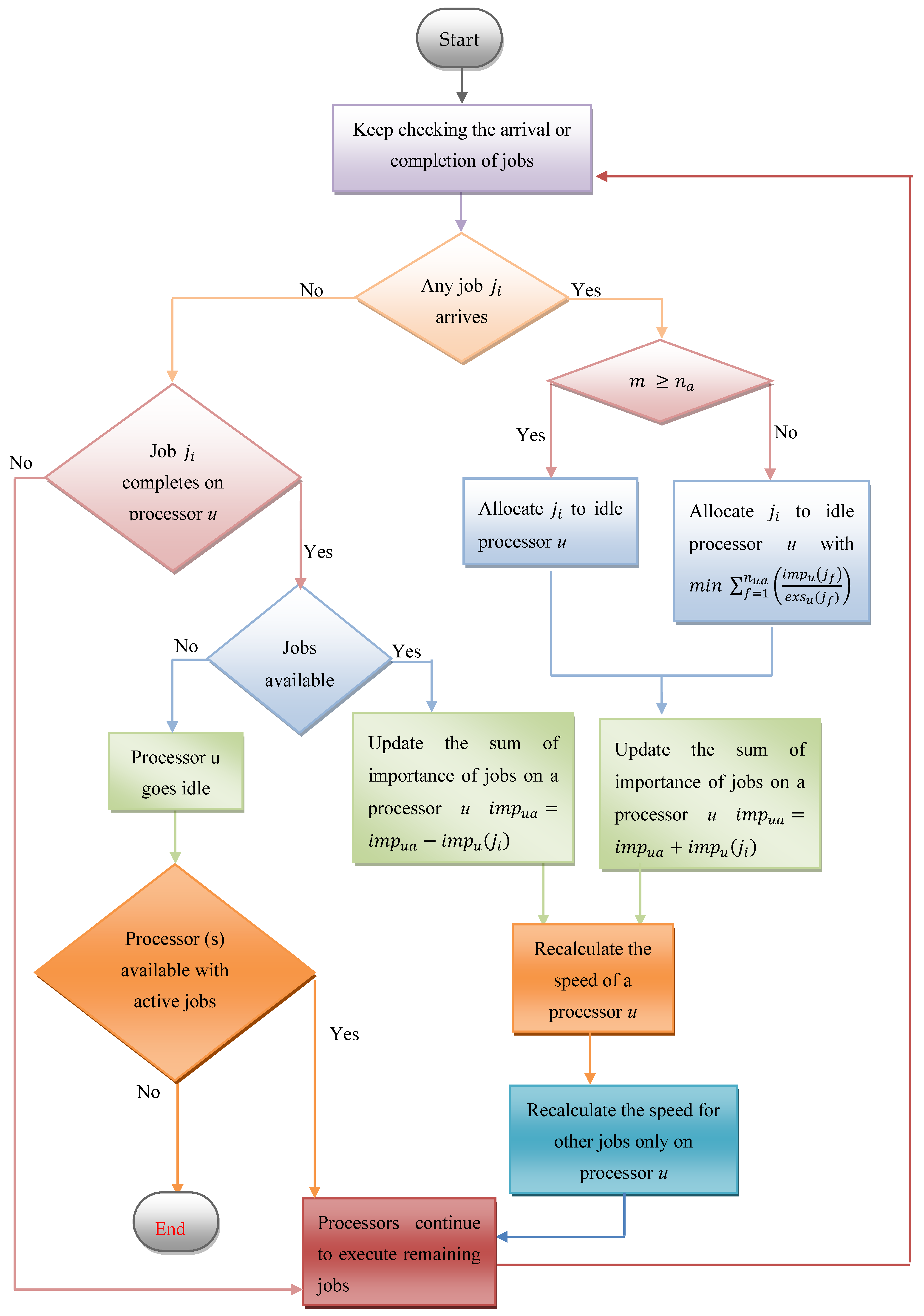
5.1. Multiprocessor with Bounded Speed Algorithm: MBS

At time t, the processing speed of u adjusts to $s_{ua}\left(t\right)=\left(1+\raisebox{1ex}{$\Delta $}\!\left/ \!\raisebox{-1ex}{$3m$}\right.\right)·min\left({\left(\frac{im{p}_{ua}\left(t\right)}{\mathsf{Ϯ}}\right)}^{\raisebox{1ex}{$1$}\!\left/ \!\raisebox{-1ex}{$\alpha $}\right.}, \eta \right)$, where $0<\Delta \le \left(\frac{1}{3\alpha }\right)$, $\mathsf{Ϯ}\ge 1$ and $\alpha \ge 2$ are constants. The importance $imp\left(j\right)$ of a job is uninformed and acknowledged only at release time $r\left(j\right)$. The policies considered for the multiprocessor scheduling MBS are as follows:

Job selection policy: The importance-based/weighted round robin is used on every processor.

Job assignment policy: a newly arrived job is allotted to an idle processor (if available) or to a processor having the minimum sum of the ratio of importance to the executed size for all jobs on that processor (i.e., $min {\sum }_{f=1}^{n_{ua}}\left(\frac{im{p}_u\left(j_f\right)}{ex{s}_u\left(j_f\right)}\right)$).

Speed scaling policy: The speed of every processor is scaled on the bases of the total importance of active jobs on that processor. Every active job $j_i$ on u obtains the fraction of speed:

$$processor’s speed\left(\frac{importance of{j}_i }{total importance of all active jobs on that processor}\right)$$

i.e., $s_{ua}·\left(\frac{im{p}_u\left(j_i\right)}{{\sum }_{k=1}^{n_{ua}}im{p}_u\left(j_k\right)}\right)$ or $s_{ua}·\left(\frac{im{p}_u\left(j_i\right)}{im{p}_{ua}}\right)$. The speed of any processor gets adjusted (re-evaluated) on alteration in total importance of active jobs on that processor. MBS is compared against an optimal offline algorithm Opt, using potential function analysis. The principal result of this study is stated in Theorem 1. The Algorithm 1 of MBS is given next and the flow chart for MBS is given in Figure 2.

Algorithm 1: MBS (Multiprocessor with Bounded Speed)

Input: total m number of processors $\left\{u_1,\dots ,u_k,\dots ,u_m\right\}$, $n_a$ NoAJ $\left\{j_1,\dots ,j_i,\dots ,j_{n_a}\right\}$ and the importance of all $n_a$ active jobs $\left\{\mathit{imp}\left(j_1\right),\dots ,\mathit{imp}\left(j_i\right),\dots ,\mathit{imp}\left(j_{n_a}\right)\right\}$. Output: number of jobs allocated to every processor, the speed of all processors, at any time and execution speed share of each active job. Repeat until all processors become idle: 1. If any job $j_i$ arrives 2. if $m\ge n_a$ 3. allocate job $j_i$ to a idle processor u 4. otherwise, when $m<n_a$ 5. allocate job $j_i$ to a processor u with $min{\sum }_{f=1}^{n_{\mathit{ua}}}\left(\frac{{\mathit{imp}}_u\left(j_f\right)}{{\mathit{exs}}_u\left(j_f\right)}\right)$ 6. ${\mathit{imp}}_{\mathit{ua}}={\mathit{imp}}_{\mathit{ua}}+{\mathit{imp}}_u\left(j_i\right)$ 7. $s_{\mathit{ua}}=\left(1+\raisebox{1ex}{$\Delta $}\!\left/ \!\raisebox{-1ex}{$3m$}\right.\right)·min\left({\left(\frac{{\mathit{imp}}_{\mathit{ua}}}{\mathsf{Ϯ}}\right)}^{\raisebox{1ex}{$1$}\!\left/ \!\raisebox{-1ex}{$\alpha $}\right.},\eta \right)$, where $0<\Delta \le \left(\frac{1}{3\alpha }\right)$ and $\mathsf{Ϯ}>1$ is a constant value 8. Otherwise, if any job $j_i$ completes on any processor u and other active jobs are available for execution on that processor then 9. ${\mathit{imp}}_{\mathit{ua}}={\mathit{imp}}_{\mathit{ua}}-{\mathit{imp}}_u\left(j_i\right)$ 10. $s_{\mathit{ua}}=\left(1+\raisebox{1ex}{$\Delta $}\!\left/ \!\raisebox{-1ex}{$3m$}\right.\right)·min\left({\left(\frac{{\mathit{imp}}_{\mathit{ua}}}{\mathsf{Ϯ}}\right)}^{\raisebox{1ex}{$1$}\!\left/ \!\raisebox{-1ex}{$\alpha $}\right.},\eta \right)$, where $0<\Delta \le \left(\frac{1}{3\alpha }\right)$ and $\mathsf{Ϯ}\ge 1$ is a constant value 11. the speed received by any job $j_i$, which is executing on a processor u, is $s_{\mathit{ua}}·\left(\frac{{\mathit{imp}}_u\left(j_i\right)}{{\mathit{imp}}_{\mathit{ua}}}\right)$ 12. otherwise, processors continue to execute remaining jobs

Theorem 1.

When using more than two processors $\left(i.e., m\ge 2\right)$ and each processor has the permitted maximum speed $\left(1+\raisebox{1ex}{$\Delta $}\!\left/ \!\raisebox{-1ex}{$3m$}\right.\right)\eta$, MBS is c-competitive for the objective of minimizing the IbFt+E, where $c=\left(\frac{9}{8}+\frac{3\Delta }{8}\right)·\left(1+{\left(1+\raisebox{1ex}{$\Delta $}\!\left/ \!\raisebox{-1ex}{$3m$}\right.\right)}^{\alpha }\right)=O\left(1\right)$ and $0<\Delta \le \frac{1}{3\alpha }$.

5.2. Necessary Conditions to be Fulfilled

A potential function is needed to calculate the c-competitiveness of an algorithm. An algorithm is called c-competitive if at any time t, the sum of augmentation in the objective cost of algorithm and the modification in the value of potential is at the most c times the augmentation in the objective cost of the optimal adversary algorithm. A potential function $\Phi \left(t\right)$ is required to demonstrate that MBS is c-competitive. A c-competitive algorithm should satisfy the conditions:

Boundary Condition: The value of potential function is zero before the release of any job and after the completion of all jobs.

Job Arrival and Completion Condition: The value of potential function remains same on arrival or completion of a job.

Running Condition: At time when the above condition do not exist, the sum of the (rate of change) RoC of $G_a$ and the RoC of $\Phi$ is at the most c times the RoC of $G_o$.

$$\frac{d{G}_a\left(t\right)}{dt}+\gamma ·\frac{d\Phi }{dt}\le c·\frac{d{G}_o\left(t\right)}{dt},\mathrm{where}\gamma >0.$$

(1)

5.3. Potential Function $\Phi \left(t\right)$

An active job j is lagging, if $\left(pw{k}_a\left(j, t\right)-pw{k}_o\left(j, t\right)\right)>0$. Since t is the instantaneous time, this factor is dropped from the rest of the analysis. For any processor u, let $L{G}_u=\left\{j_1, j_2, \dots , j_{l{g}_u}\right\}$ be a group of lagging jobs using MBS and these jobs are managed in the ascending order of latest time (when any job gets changed into lagging job). $LG={\sum }_{u=1}^{m}L{G}_u$ is a set of all lagging jobs on all m processors. Further, $im{p}_{l{g}_u}={\sum }_{i=1}^{l{g}_u}im{p}_u\left(j_i\right)$ is the sum of the importance of lagging jobs on a processor u. Following this, $im{p}_{lg}={\sum }_{u=1}^{m}im{p}_{l{g}_u}$ is the sum of the importance of lagging jobs on all m processors. Our potential function $\Phi \left(t\right)$ for IbFt+E is the addition of all potential values of m processors.

$$\Phi \left(t\right)={\displaystyle \sum }_{u=1}^m{\Phi }_u\left(t\right)$$

(2)

$${\Phi }_u\left(t\right)=\{\begin{array}{l}{\sum }_{i=1}^{l{g}_u}\left({\left({\sum }_{k=1}^{i}im{p}_u\left(j_k\right)\right)}^{1-2\delta }\right)·{\omega }_i\hspace{1em}\hspace{1em}if {\sum }_{k=1}^{i}im{p}_u\left(j_k\right) \le {\eta }^{\raisebox{1ex}{$1$}\!\left/ \!\raisebox{-1ex}{$2\delta $}\right.}\\ {\sum }_{i=1}^{l{g}_u}\left(\frac{1}{1-\delta }\right)·\left({\sum }_{k=1}^{i}im{p}_u\left(j_k\right)·{\eta }^{-1}\right)·{\omega }_i\hspace{1em}\hspace{1em}otherwise\end{array}$$

(3)

$$\begin{array}{c}\mathit{Where}\hspace{1em}{\omega }_i=max\left\{0, \left(pw{k}_a\left(j_i, t\right)-pw{k}_o\left(j_i, t\right)\right)\right\}\\ \delta =\raisebox{1ex}{$1$}\!\left/ \!\raisebox{-1ex}{$2\alpha $}\right.\mathrm{and}\end{array}$$

(4)

$${\left({\sum }_{k=1}^{i}im{p}_u\left(j_k\right)\right)}^{1-2\delta }\mathrm{and}\left(\frac{1}{1-\delta }\right)·\left({\sum }_{k=1}^{i}im{p}_u\left(j_k\right)·{\eta }^{-1}\right)$$

(5)

are the coefficients c_i of j_i on processor u

MBS is analyzed per machine basis. Firstly, the verification of boundary condition: the value of $\Phi$ is zero after finishing of all jobs and prior to release of any job on any processor. There will be no active job on any processor in both situations. Therefore, the boundary condition is true. Secondly, the verification of arrival and completion condition: at time t, on release of a new job $j_i$ in I, $j_i$ without execution is appended at end of I. ${\omega }_i$ is zero as $pw{k}_a\left(j_i, t\right)-pw{k}_o\left(j_i, t\right)=0$. The coefficient of all other jobs does not change and $\Phi$ remains unchanged. At the time of completion of a job $j_i$, ${\omega }_i$ becomes zero and other coefficients of lagging jobs either remains unchanged or decreases, so, $\Phi$ does not increase. Thus the arrival and completion criteria holds true. The third and last criterion to confirm is running condition, with no job arrival or completion.

According to previous discussion, for any processor u, let $\frac{d{G}_{ua}}{dt}=im{p}_{ua}+s_{ua}{}^{\alpha }$ and $\frac{d{G}_{uo}}{dt}=im{p}_{uo}+s_{uo}{}^{\alpha }$ be the alteration of IbFt+E in an infinitesimal period of time $\left[t, t+dt\right]$ by MBS and Opt, respectively. The alteration of $\Phi$ because of Opt and MBS in an infinitesimal period of time $\left[t, t+dt\right]$ by u is $\frac{d{\Phi }_{uo}}{dt}$ and $\frac{d{\Phi }_{ua}}{dt}$, respectively. The whole alteration in $\Phi$ because of Opt and MBS in infinitesimal period of time $\left[t, t+dt\right]$ by u is $\frac{d{\Phi }_u}{dt}=\frac{d{\Phi }_{uo}}{dt}+\frac{d{\Phi }_{ua}}{dt}$. As this is multiprocessor system therefore to bound the RoC of $\Phi$ by Opt and MBS, the analysis is divided in two cases based on $n_a$ and $m$, and then every case is further divided in three sub cases depending on whether $im{p}_{ua}>{\eta }^{\alpha }$ and $im{p}_{l_u}>{\eta }^{\alpha }$, afterwards each sub case is further divided in two sub cases depending on $im{p}_{lg}>\left(im{p}_a-\left(\frac{3}{3+\Delta }\right)·im{p}_a\right)$ and $im{p}_{lg}\le \left(im{p}_a-\left(\frac{3}{3+\Delta }\right)·im{p}_a\right)$, where $0<\Delta <1$, $\mu =\frac{3}{3+\Delta }$. The potential analysis is done on individual processor basis, the reason behind it is that all the processors will not face the same case at the same time; rather different processors may face same or different cases.

Lemma 1.

For the positive real numbers x, y, A and B, if $x^{-1}+y^{-1}=1$ holds then [2]:

$$x^{-1}·A^x+y^{-1}·B^y\ge A·B$$

(6)

Lemma 2.

If $n_a\le m$ and $im{p}_{l{g}_u}\le {\eta }^{\alpha }$

(a) $\frac{d{\Phi }_{uo}}{dt}\le \frac{s_{uo}{}^{\alpha }}{\alpha }+\left(1-2\delta \right)·im{p}_{l{g}_u}$; (b) $\frac{d{\Phi }_{ua}}{dt}\le -\left(s_{ua}·im{p}_{l{g}_u}{}^{1-2\delta }\right)$

Proof. 

If $n_a\le m$ then every processor executes not more than one job, i.e., every job is processed on individual processor.

(a) It is required to upper-bound $\frac{d{\Phi }_{uo}}{dt}$ for a processor u. To calculate the upper-bound, the worst-case is considered which occurs if Opt executes a job on u with the largest coefficient $c_{l{g}_u}=im{p}_{l{g}_u}{}^{1-2\delta }$. At this time, ${\omega }_i$ increases at the rate of $s_{uo}$ (because of Opt on u). The count of lagging jobs on some u may be only one.

$$\frac{d{\Phi }_{uo}}{dt}\le c_{l{g}_u}·s_{uo}\le im{p}_{l{g}_u}{}^{1-2\delta }·s_{uo}$$

(7)

Using Young’s inequality, Lemma 1 (Equation (6)) in (7) such that A = $s_{uo}$, B = ${\left(im{p}_{l{g}_u}\right)}^{1-2\delta }$, x = $\alpha$ and y = $\frac{1}{1-2\delta }$ we have:

$$\frac{d{\Phi }_{uo}}{dt}\le \frac{s_{uo}{}^{\alpha }}{\alpha }+\left(1-2\delta \right)·im{p}_{l{g}_u}$$

(8)

(b) Next, it is required to upper-bound $\frac{d{\Phi }_{ua}}{dt}$ for a processor u. To compute the upper-bound, consider that a lagging job $j_i$ on u is executed at the rate of $\left(s_{ua}·\frac{im{p}_u\left(j_i\right)}{{\sum }_{k=1}^{n_{ua}}im{p}_u\left(j_k\right)}\right)$ or $\left(s_{ua}·\frac{im{p}_u\left(j_i\right)}{im{p}_{ua}}\right)$, therefore, the change in ${\omega }_i$ is at the rate of $\left(-s_{ua}·\frac{im{p}_u\left(j_i\right)}{im{p}_{ua}}\right)$.

$$\frac{d{\Phi }_{ua}}{dt}={\sum }_{i=1}^{l{g}_u}\left({\left({\sum }_{k=1}^{i}im{p}_u\left(j_k\right)\right)}^{1-2\delta }\right)·\left(-s_{ua}·\frac{im{p}_u\left(j_i\right)}{im{p}_{ua}}\right)$$

As only one job executes on a processor, therefore $\frac{im{p}_u\left(j_i\right)}{im{p}_{ua}}=1$ and $l{g}_u=i=1$,

$$\begin{array}{c}\frac{d{\Phi }_{ua}}{dt}=\left(im{p}_{l{g}_u}{}^{1-2\delta }\right)·\left(-s_{ua}\right)\\ \frac{d{\Phi }_{ua}}{dt}=-\left(s_{ua}·im{p}_{l{g}_u}{}^{1-2\delta }\right)\end{array}$$

(9)

□

Lemma 3.

If $n_a\le m$ and $im{p}_{l{g}_u}>{\eta }^{\alpha }$

(a) $\frac{d{\Phi }_{uo}}{dt}\le \left(\frac{1}{1-\delta }\right)·im{p}_{l{g}_u}$; (b) $\frac{d{\Phi }_{ua}}{dt}=-\frac{\left(1+\raisebox{1ex}{$\Delta $}\!\left/ \!\raisebox{-1ex}{$3m$}\right.\right)}{\left(1-\delta \right)}·im{p}_{l{g}_u}$

Proof. 

If $n_a\le m$ then every processor executes not more than one job, i.e., every job is processed on individual processor.

(a) It is required to upper-bound $\frac{d{\Phi }_{uo}}{dt}$ for a processor u. To calculate the upper-bound, the worst-case is considered which occurs if Opt executes a job on u with the largest coefficient $c_{l{g}_u}=\left(\frac{1}{1-\delta }\right)·im{p}_{l{g}_u}·{\eta }^{-1}$. At this time, ${\omega }_i$ increases at the rate of $s_{uo}$ (because of Opt on u) where $s_{uo}\le \eta$. The count of lagging jobs on any u may be only one.

$$\begin{array}{c}\frac{d{\Phi }_{uo}}{dt}\le c_{l{g}_u}·s_{uo}\le c_{l{g}_u}·\eta =\left(\frac{1}{1-\delta }\right)·im{p}_{l{g}_u}·{\eta }^{-1}·\eta \\ \frac{d{\Phi }_{uo}}{dt}\le \left(\frac{1}{1-\delta }\right)·im{p}_{l{g}_u}\end{array}$$

(10)

(b) Next, it is required to upper-bound $\frac{d{\Phi }_{ua}}{dt}$ for a processor u. To compute the upper-bound, consider that a lagging job $j_i$ on u is executed at the rate of $\left(s_{ua}·\frac{im{p}_u\left(j_i\right)}{{\sum }_{k=1}^{n_{ua}}im{p}_u\left(j_k\right)}\right)$ or $\left(s_{ua}·\frac{im{p}_u\left(j_i\right)}{im{p}_{ua}}\right)$, therefore the change in ${\omega }_i$ is at the rate of $\left(-s_{ua}·\frac{im{p}_u\left(j_i\right)}{im{p}_{ua}}\right)$. $im{p}_{ua}\ge im{p}_{g{l}_u}>{\eta }^{\alpha }$, $s_{ua}=\left(1+\raisebox{1ex}{$\Delta $}\!\left/ \!\raisebox{-1ex}{$3m$}\right.\right)·\eta$

$$\frac{d{\Phi }_{ua}}{dt}={\sum }_{i=1}^{l{g}_u}\left(\frac{1}{1-\delta }\right)·\left({{\displaystyle \sum }}_{k=1}^{i}im{p}_u\left(j_k\right)·{\eta }^{-1}\right)·\left(-s_{ua}·\frac{im{p}_u\left(j_i\right)}{im{p}_{ua}}\right)$$

As only one job executes on a processor, therefore $\frac{im{p}_u\left(j_i\right)}{im{p}_{ua}}=1$ and $l{g}_u=i=1$,

$$\begin{array}{ll}\frac{d{\Phi }_{ua}}{dt}& =\left(\frac{1}{1-\delta }\right)·\left(im{p}_{l{g}_u}·{\eta }^{-1}\right)·\left(-s_{ua}\right)\\ & =-\left(\frac{1}{1-\delta }\right)·\left(s_{ua}·im{p}_{l{g}_u}·{\eta }^{-1}\right)\\ & =-\left(\frac{1}{1-\delta }\right)·\left(\left(1+\raisebox{1ex}{$\Delta $}\!\left/ \!\raisebox{-1ex}{$3m$}\right.\right)·\eta ·im{p}_{l{g}_u}·{\eta }^{-1}\right)\end{array}$$

$$\frac{d{\Phi }_{ua}}{dt}=-\frac{\left(1+\raisebox{1ex}{$\Delta $}\!\left/ \!\raisebox{-1ex}{$3m$}\right.\right)}{\left(1-\delta \right)}·im{p}_{l{g}_u}$$

(11)

□

Lemma 4.

If $n_a>m$ and $im{p}_{l{g}_u}\le {\eta }^{\alpha }$

(a) $\frac{d{\Phi }_{uo}}{dt}\le \frac{s_{uo}{}^{\alpha }}{\alpha }+\left(1-2\delta \right)·im{p}_{l{g}_u}$; (b) $\frac{d{\Phi }_{ua}}{dt}\le -\frac{s_{ua}}{\left(2-2\delta \right)}·\left(\frac{im{p}_{l{g}_u}{}^{2-2\delta }}{im{p}_{ua}}\right)$

Proof. If $n_a>m$ then:

(a) It is required to upper-bound $\frac{d{\Phi }_{uo}}{dt}$ for a processor u. To calculate the upper-bound, the worst-case is considered which occurs if Opt is executing a job on u with the largest coefficient $c_{l{g}_u}=im{p}_{l{g}_u}{}^{1-2\delta }$. At this time, ${\omega }_i$ increases at the rate of $s_{uo}$ (because of Opt on u).

$$\frac{d{\Phi }_{uo}}{dt}\le c_{l{g}_u}·s_{uo}=im{p}_{l{g}_u}{}^{1-2\delta }·s_{uo}$$

(12)

Using Young’s inequality, Lemma 1 (Equation (6)) in (12) such that A = $s_{uo}$ , B = $im{p}_{l{g}_u}{}^{1-2\delta }$, x = $\alpha$ and y = $\frac{1}{1-2\delta }$ we have:

$$\frac{d{\Phi }_{uo}}{dt}\le \frac{s_{uo}{}^{\alpha }}{\alpha }+\left(1-2\delta \right)·im{p}_{l{g}_u}$$

(13)

(b) Next, it is required to upper-bound $\frac{d{\Phi }_{ua}}{dt}$ for a processor u, to compute the upper-bound consider that a lagging job $j_i$ on u is executed at the rate of $\left(s_{ua}·\frac{im{p}_u\left(j_i\right)}{{\sum }_{k=1}^{n_{ua}}im{p}_u\left(j_k\right)}\right)$ or $\left(s_{ua}·\frac{im{p}_u\left(j_i\right)}{im{p}_{ua}}\right)$, therefore the change in ${\omega }_i$ is at the rate of $\left(-s_{ua}·\frac{im{p}_u\left(j_i\right)}{im{p}_{ua}}\right)$. To make the discussion straightforward, let $h_{ui}={\sum }_{k=1}^{i}im{p}_u\left(j_k\right)$, $h_{u0}=0$, $h_{ul{g}_u}=im{p}_{l{g}_u}$ and $im{p}_u\left(j_i\right)=h_{ui}-h_{ui-1}$. (by using Equation (3):

$$\begin{array}{ll}\frac{d{\Phi }_{ua}}{dt}& ={\sum }_{i=1}^{l{g}_u}\left({\left({\sum }_{k=1}^{i}im{p}_u\left(j_k\right)\right)}^{1-2\delta }\right)·\left(-s_{ua}·\frac{im{p}_u\left(j_i\right)}{im{p}_{ua}}\right)\\ & =-\frac{s_{ua}}{im{p}_{ua}}{\sum }_{i=1}^{l{g}_u}\left({\left(h_{ui}\right)}^{1-2\delta }\right)·\left(h_{ui}-h_{ui-1}\right)\\ & \le -\frac{s_{ua}}{im{p}_{ua}}{\sum }_{i=1}^{l{g}_u}{{\displaystyle \int }}_{h_{ui-1}}^{h_{ui}}{f}^{1-2\delta }df\\ & \le -\frac{s_{ua}}{im{p}_{ua}}{{\displaystyle \int }}_0^{h_{ul{g}_u}}{f}^{1-2\delta }df\\ & =-\frac{s_{ua}}{im{p}_{ua}}·\frac{h_{ul{g}_u}{}^{2-2\delta }}{\left(2-2\delta \right)}\\ & =-\frac{s_{ua}}{im{p}_{ua}}·\frac{im{p}_{l{g}_u}{}^{2-2\delta }}{\left(2-2\delta \right)}\end{array}$$

$$\frac{d{\Phi }_{ua}}{dt}\le -\frac{s_{ua}}{\left(2-2\delta \right)}·\left(\frac{im{p}_{l{g}_u}{}^{2-2\delta }}{im{p}_{ua}}\right)$$

(14)

□

Lemma 5.

If $n_a>m$ and $im{p}_{l{g}_u}>{\eta }^{\alpha }$

(a) $\frac{d{\Phi }_{uo}}{dt}\le \left(\frac{1}{1-\delta }\right)·im{p}_{l{g}_u}$; (b) $\frac{d{\Phi }_{ua}}{dt}\le -\frac{\left(1+\raisebox{1ex}{$\Delta $}\!\left/ \!\raisebox{-1ex}{$3m$}\right.\right)}{\left(2-2\delta \right)}·\left(\frac{im{p}_{l{g}_u}{}^2}{im{p}_{ua}}\right)$

Proof. 

If $n_a>m$ then:

(a) It is required to upper-bound $\frac{{d\Phi }_{\mathrm{uo}}}{\mathit{dt}}$ for a processor u. To calculate the upper-bound, the worst-case is considered which occurs if Opt executes a job on u with the largest coefficient $c_{{\mathit{lg}}_u}=\left(\frac{1}{1-\delta }\right)·{\mathit{imp}}_{{\mathit{lg}}_u}·{\eta }^{-1}$ (as ${\mathit{imp}}_{\mathit{ua}}\ge {\mathit{imp}}_{{\mathit{lg}}_u}>{\eta }^{\alpha }$). At this time, ${\omega }_i$ increases at the rate of $s_{uo}$ (because of Opt on u).

$$\begin{array}{ll}\frac{d{\Phi }_{uo}}{dt}& \le c_{l{g}_u}·s_{uo}\\ & =\left(\frac{1}{1-\delta }\right)·im{p}_{l{g}_u}·{\eta }^{-1}·s_{uo}\\ & \le \left(\frac{1}{1-\delta }\right)·im{p}_{l{g}_u}·{\eta }^{-1}·\eta \hspace{1em}\hspace{1em}\left\{\because s_{uo}\le \eta \right\}\end{array}$$

$$\frac{d{\Phi }_{uo}}{dt}\le \left(\frac{1}{1-\delta }\right)·im{p}_{l{g}_u}$$

(15)

(b) Next, it is required to upper-bound $\frac{d{\Phi }_{ua}}{dt}$ for a processor u. To compute the upper-bound, consider that a lagging job $j_i$ on u is executed at the rate of $\left(s_{ua}·\frac{im{p}_u\left(j_i\right)}{{{\displaystyle \sum }}_{k=1}^{n_{ua}}im{p}_u\left(j_k\right)}\right)$ or $\left(s_{ua}·\frac{im{p}_u\left(j_i\right)}{im{p}_{ua}}\right)$, therefore the change in ${\omega }_i$ is at the rate of $\left(-s_{ua}·\frac{im{p}_u\left(j_i\right)}{im{p}_{ua}}\right)$. To make the discussion uncomplicated, let $h_{ui}={{\displaystyle \sum }}_{k=1}^{i}im{p}_u\left(j_k\right)$, $h_{u0}=0$, $h_{ul{g}_u}=im{p}_{l{g}_u}>{\eta }^{\alpha }$, $im{p}_{ua}\ge im{p}_{l{g}_u}>{\eta }^{\alpha }$ and $im{p}_u\left(j_i\right)=h_{ui}-h_{ui-1}$. Let z < $l_u$ be the largest integer such that $h_{u_z}\le {\eta }^{\alpha }$. (using Equation (3)):

$$\begin{array}{ll}\frac{d{\Phi }_{ua}}{dt}& ={\sum }_{i=1}^{l{g}_u}{c}_i·\left(-s_{ua}·\frac{im{p}_u\left(j_i\right)}{im{p}_{ua}}\right)\\ & =-\left(\frac{s_{ua}}{im{p}_{ua}}\right)·\left({{\displaystyle \sum }}_{i=1}^z\left(im{p}_u\left(j_i\right)·{\left(h_{ui}\right)}^{1-2\delta }\right)+{{\displaystyle \sum }}_{i=z+1}^{l{g}_u}\left(\left(\frac{1}{1-\delta }\right)·\left(im{p}_u\left(j_i\right)·h_{ui}·{\eta }^{-1}\right)\right)\right)\\ & \le -\left(\frac{s_{ua}}{im{p}_{ua}}\right)·\left(\left({{\displaystyle \int }}_0^{h_{u_z}}{f}^{1-2\delta }df\right)+\left(\left(\frac{1}{1-\delta }\right)·{\eta }^{-1}·\left({{\displaystyle \int }}_{h_{u_z}}^{h_{ul{g}_u}}fdf\right)\right)\right)\\ & =-\left(\frac{s_{ua}}{im{p}_{ua}}\right)·\left(\frac{h_{u_z}{}^{2-2\delta }}{\left(2-2\delta \right)}+\frac{h_{ul{g}_u}{}^2-h_{u_z}{}^2}{\left(2-2\delta \right)·\eta }\right)\\ & =-\left(\frac{s_{ua}}{im{p}_{ua}}\right)·\left(\frac{h_{u_z}{}^2}{\left(2-2\delta \right)h_{u_z}{}^{\raisebox{1ex}{$1$}\!\left/ \!\raisebox{-1ex}{$\alpha $}\right.}}+\frac{h_{ul{g}_u}{}^2-h_{u_z}{}^2}{\left(2-2\delta \right)·\eta }\right)\\ & \le -\frac{\left(1+\raisebox{1ex}{$\Delta $}\!\left/ \!\raisebox{-1ex}{$3m$}\right.\right)·\eta }{im{p}_{ua}}·\left(\frac{h_{u_z}{}^2}{\left(2-2\delta \right)\eta }+\frac{h_{ul{g}_u}{}^2-h_{u_z}{}^2}{\left(2-2\delta \right)·\eta }\right)\hspace{1em}\left\{\because h_{u_z}\le {\eta }^{\alpha }\right\}\\ & =-\frac{\left(1+\raisebox{1ex}{$\Delta $}\!\left/ \!\raisebox{-1ex}{$3m$}\right.\right)}{im{p}_{ua}}·\frac{h_{ul{g}_u}{}^2}{\left(2-2\delta \right)}\\ & =-\frac{\left(1+\raisebox{1ex}{$\Delta $}\!\left/ \!\raisebox{-1ex}{$3m$}\right.\right)}{\left(2-2\delta \right)}·\left(\frac{im{p}_{l{g}_u}{}^2}{im{p}_{ua}}\right)\end{array}$$

$$\frac{d{\Phi }_{ua}}{dt}\le -\frac{\left(1+\raisebox{1ex}{$\Delta $}\!\left/ \!\raisebox{-1ex}{$3m$}\right.\right)}{\left(2-2\delta \right)}·\left(\frac{im{p}_{l{g}_u}{}^2}{im{p}_{ua}}\right)$$

(16)

□

Lemma 6. At all time t, when $\Phi$ does not comprise discrete alteration $\frac{{\mathit{dG}}_{\mathit{ua}}}{\mathit{dt}}+\gamma ·\frac{{d\Phi }_u}{\mathit{dt}}\le c·\frac{{\mathit{dG}}_{\mathit{uo}}}{\mathit{dt}}$, where $c=\left(\frac{9}{8}+\frac{3\Delta }{8}\right)·\left(1+{\left(1+\raisebox{1ex}{$\Delta $}\!\left/ \!\raisebox{-1ex}{$3m$}\right.\right)}^{\alpha }\right)$. Assume that $\gamma =\frac{1}{16}·\left(1+{\left(1+\raisebox{1ex}{$\Delta $}\!\left/ \!\raisebox{-1ex}{$3m$}\right.\right)}^{\alpha }\right)$.

Proof. 

The analysis is divided in two cases based on $n_a>m$ or $n_a\le m$, and then each case is again alienated in three sub-cases depending on whether $im{p}_{ua}>{\eta }^{\alpha }$ or $im{p}_{ua}\le {\eta }^{\alpha }$ and $im{p}_{l{g}_u}>{\eta }^{\alpha }$ or $im{p}_{l{g}_u}\le {\eta }^{\alpha }$, afterwards each sub-case is again alienated in two sub-cases depending on whether $im{p}_{l{g}_u }>\left(im{p}_{ua}-\left(\frac{3}{3+\Delta }\right)·im{p}_{ua}\right)$ or $im{p}_{l{g}_u }\le \left(im{p}_{ua}-\left(\frac{3}{3+\Delta }\right)·im{p}_{ua}\right)$, where $0<\mu =\left(\frac{3}{3+\Delta }\right)<1$ and $\Delta =\left(\raisebox{1ex}{$1$}\!\left/ \!\raisebox{-1ex}{$3\alpha $}\right.\right)$. As a job in MBS which is not lagging must be an active job in Opt,

$$im{p}_{uo }\ge im{p}_{ua}-im{p}_{l{g}_u}\ge im{p}_{ua}-\left(im{p}_{ua}-\mu ·im{p}_{ua}\right)\ge \mu im{p}_{ua}\Rightarrow im{p}_{ua} \le \frac{im{p}_{uo }}{\mu }$$

(17)

$$\mu =\left(\frac{3}{3+\Delta }\right)$$

(18)

$$\gamma =\frac{1}{16}·\left(1+{\left(1+\raisebox{1ex}{$\Delta $}\!\left/ \!\raisebox{-1ex}{$3m$}\right.\right)}^{\alpha }\right)$$

(19)

$$c=\left(\frac{9}{8}+\frac{3\Delta }{8}\right)·\left(1+{\left(1+\raisebox{1ex}{$\Delta $}\!\left/ \!\raisebox{-1ex}{$3m$}\right.\right)}^{\alpha }\right)$$

(20)

□

Case I: When $n_a\le m$ and $im{p}_{ua}\le {\eta }^{\alpha }$, since $im{p}_{l{g}_u}\le im{p}_{ua}$ we have $im{p}_{l{g}_u}\le {\eta }^{\alpha },$ and $s_{ua}\left(t\right)=\left(1+\raisebox{1ex}{$\Delta $}\!\left/ \!\raisebox{-1ex}{$3m$}\right.\right)·min\left(im{p}_{ua}{}^{\raisebox{1ex}{$1$}\!\left/ \!\raisebox{-1ex}{$\alpha $}\right.},\eta \right)=\left(1+\raisebox{1ex}{$\Delta $}\!\left/ \!\raisebox{-1ex}{$3m$}\right.\right)·im{p}_{ua}{}^{\raisebox{1ex}{$1$}\!\left/ \!\raisebox{-1ex}{$\alpha $}\right.}$.

(a) If $im{p}_{l{g}_u}>\left(im{p}_{ua}-\left(\frac{3}{3+\Delta }\right)·im{p}_{ua}\right)$ then the total RoC of Φ because of Opt and MBS is $\frac{d{\Phi }_u}{dt}=\frac{d{\Phi }_{uo}}{dt}+\frac{d{\Phi }_{ua}}{dt}$.

(using Equations (8) and (9))

$$\frac{d{\Phi }_u}{dt}\le \left(\frac{s_{uo}{}^{\alpha }}{\alpha }+\left(1-2\delta \right)·im{p}_{l{g}_u}\right)-\left(s_{ua}·im{p}_{l{g}_u}{}^{1-2\delta }\right)$$

(21)

(by using Equations (1) and (21))

$\frac{d{G}_{ua}}{dt}+\gamma ·\frac{d{\Phi }_u}{dt}$

$\le \left(im{p}_{ua}+s_{ua}{}^{\alpha }+\gamma ·\left(\left(\frac{s_{uo}{}^{\alpha }}{\alpha }+\left(1-2\delta \right)·im{p}_{l{g}_u}\right)-\left(s_{ua}·im{p}_{l{g}_u}{}^{1-2\delta }\right)\right)\right)$

$=\left(im{p}_{ua}+{\left(1+\raisebox{1ex}{$\Delta $}\!\left/ \!\raisebox{-1ex}{$3m$}\right.\right)}^{\alpha }·im{p}_{ua}+\frac{\gamma }{\alpha }·s_{uo}{}^{\alpha }+\gamma ·\left(1-2\delta \right)·im{p}_{l{g}_u}-\gamma ·\left(1+\raisebox{1ex}{$\Delta $}\!\left/ \!\raisebox{-1ex}{$3m$}\right.\right)·im{p}_{ua}{}^{\raisebox{1ex}{$1$}\!\left/ \!\raisebox{-1ex}{$\alpha $}\right.}·im{p}_{l{g}_u}{}^{1-2\delta }\right)$

$\le \left(\frac{\gamma }{\alpha }·s_{uo}{}^{\alpha }+\left(1+{\left(1+\raisebox{1ex}{$\Delta $}\!\left/ \!\raisebox{-1ex}{$3m$}\right.\right)}^{\alpha }\right)·im{p}_{ua}+\gamma ·\left(1-2\delta \right)·im{p}_{ua}-\gamma ·\left(1+\raisebox{1ex}{$\Delta $}\!\left/ \!\raisebox{-1ex}{$3m$}\right.\right)·im{p}_{ua}{}^{\raisebox{1ex}{$1$}\!\left/ \!\raisebox{-1ex}{$\alpha $}\right.}·{\left(\left(1-\left(\frac{3}{3+\Delta }\right)\right)·im{p}_{ua}\right)}^{1-2\delta }\right)$

$=\left(\frac{\gamma }{\alpha }·s_{uo}{}^{\alpha }+im{p}_{ua}·\left(1+{\left(1+\raisebox{1ex}{$\Delta $}\!\left/ \!\raisebox{-1ex}{$3m$}\right.\right)}^{\alpha }+\gamma ·\left(1-2\delta \right)-\gamma ·\left(1+\raisebox{1ex}{$\Delta $}\!\left/ \!\raisebox{-1ex}{$3m$}\right.\right)·{\left(\frac{\Delta }{3+\Delta }\right)}^{1-2\delta }\right)\right)$

$\le \frac{\gamma }{\alpha }·s_{uo}{}^{\alpha }+im{p}_{ua}·\left(1+{\left(1+\raisebox{1ex}{$\Delta $}\!\left/ \!\raisebox{-1ex}{$3m$}\right.\right)}^{\alpha }+\gamma -\gamma ·{\left(\frac{\Delta }{3+\Delta }\right)}^{1-2\delta }\right)$

$\le \frac{\gamma }{\alpha }·s_{uo}{}^{\alpha }+im{p}_{ua}·\left(1+{\left(1+\raisebox{1ex}{$\Delta $}\!\left/ \!\raisebox{-1ex}{$3m$}\right.\right)}^{\alpha }+\gamma -\gamma ·\left(\frac{\Delta }{3+\Delta }\right)\right)$

$=\frac{\gamma }{\alpha }·s_{uo}{}^{\alpha }+im{p}_{ua}·\left(1+{\left(1+\raisebox{1ex}{$\Delta $}\!\left/ \!\raisebox{-1ex}{$3m$}\right.\right)}^{\alpha }+\gamma ·\left(\frac{3}{3+\Delta }\right)\right)$

$\le \frac{\gamma }{\alpha }·s_{uo}{}^{\alpha }+im{p}_{ua}·\left(1+{\left(1+\raisebox{1ex}{$\Delta $}\!\left/ \!\raisebox{-1ex}{$3m$}\right.\right)}^{\alpha }+\gamma \right)$

$=\frac{\gamma }{\alpha }·s_{uo}{}^{\alpha }+im{p}_{ua}·\left(1+{\left(1+\raisebox{1ex}{$\Delta $}\!\left/ \!\raisebox{-1ex}{$3m$}\right.\right)}^{\alpha }+\frac{1}{16}·\left(1+{\left(1+\raisebox{1ex}{$\Delta $}\!\left/ \!\raisebox{-1ex}{$3m$}\right.\right)}^{\alpha }\right)\right)$  (by using Equation (19))

$\le \frac{\gamma }{\alpha }·s_{uo}{}^{\alpha }+\frac{im{p}_{uo}}{\mu }·\left(\frac{17}{16}·\left(1+{\left(1+\raisebox{1ex}{$\Delta $}\!\left/ \!\raisebox{-1ex}{$3m$}\right.\right)}^{\alpha }\right)\right)$  (by using Equation (17))

$=\frac{\gamma }{\alpha }·s_{uo}{}^{\alpha }+im{p}_{uo}·\left(\frac{17}{16}·\left(1+\frac{\Delta }{3}\right)·\left(1+{\left(1+\raisebox{1ex}{$\Delta $}\!\left/ \!\raisebox{-1ex}{$3m$}\right.\right)}^{\alpha }\right)\right)$  (by using Equation (18))

$\le \frac{\gamma }{\alpha }·s_{uo}{}^{\alpha }+im{p}_{uo}·\left(\left(\frac{9}{8}+\frac{3\Delta }{8}\right)·\left(1+{\left(1+\raisebox{1ex}{$\Delta $}\!\left/ \!\raisebox{-1ex}{$3m$}\right.\right)}^{\alpha }\right)\right)$  (by using Equation (20))

$$\frac{d{G}_{ua}}{dt}+\gamma ·\frac{d{\Phi }_u}{dt}\le \frac{\gamma }{\alpha }·s_{uo}{}^{\alpha }+im{p}_{uo }·c$$

(22)

Since $c=\left(\frac{9}{8}+\frac{3\Delta }{8}\right)·\left(1+{\left(1+\raisebox{1ex}{$\Delta $}\!\left/ \!\raisebox{-1ex}{$3m$}\right.\right)}^{\alpha }\right)$ and $\gamma =\frac{1}{16}·\left(1+{\left(1+\raisebox{1ex}{$\Delta $}\!\left/ \!\raisebox{-1ex}{$3m$}\right.\right)}^{\alpha }\right)$, we have

$$\Rightarrow c=\left(\frac{9}{8}+\frac{3\Delta }{8}\right)·16\gamma \Rightarrow \frac{\gamma }{c}=\frac{1}{18+6\Delta }<1\Rightarrow \frac{\gamma }{c}<1\Rightarrow \gamma <c$$

$$\mathrm{Since}\gamma <c\mathrm{and}\alpha >1\Rightarrow 1>\frac{1}{\alpha }\Rightarrow \frac{\gamma }{\alpha }<c$$

(23)

(by using Equation (23) in Equation (22))

$$\frac{d{G}_{ua}}{dt}+\gamma ·\frac{d{\Phi }_u}{dt}\le c·s_{uo}{}^{\alpha }+c·im{p}_{uo}=c·\left(s_{uo}{}^{\alpha }+im{p}_{uo}\right)=c·\frac{d{G}_{uo}}{dt}$$

Hence the running condition is fulfilled for $n_a\le m$, $im{p}_{ua}\le {\eta }^{\alpha }$, $im{p}_{l{g}_u}\le {\eta }^{\alpha }$, $im{p}_{l{g}_u}>\left(im{p}_{ua}-\left(\frac{3}{3+\Delta }\right)·im{p}_{ua}\right)$, $c=\left(\frac{9}{8}+\frac{3\Delta }{8}\right)·\left(1+{\left(1+\raisebox{1ex}{$\Delta $}\!\left/ \!\raisebox{-1ex}{$3m$}\right.\right)}^{\alpha }\right)$.

(b) If $im{p}_{l{g}_u}\le \left(im{p}_{ua}-\left(\frac{3}{3+\Delta }\right)·im{p}_{ua}\right)$ then the total RoC of Φ because of Opt and MBS depends on $\frac{d{\Phi }_{uo}}{dt}$ since $\frac{d{\Phi }_{ua}}{dt}\le 0$.

(by using Equation (8))

$$\frac{d{\Phi }_u}{dt}\le \left(\frac{s_{uo}{}^{\alpha }}{\alpha }+\left(1-2\delta \right)·im{p}_{l{g}_u}\right)$$

(24)

(by using Equations (1) and (24))

$\frac{d{G}_{ua}}{dt}+\gamma ·\frac{d{\Phi }_u}{dt}\le im{p}_{ua}+s_{ua}{}^{\alpha }+\gamma ·\left(\frac{s_{uo}{}^{\alpha }}{\alpha }+\left(1-2\delta \right)·im{p}_{l{g}_u}\right)$

$=im{p}_{ua}+{\left(1+\raisebox{1ex}{$\Delta $}\!\left/ \!\raisebox{-1ex}{$3m$}\right.\right)}^{\alpha }·im{p}_{ua}+\frac{\gamma }{\alpha }·s_{uo}{}^{\alpha }+\gamma ·\left(1-2\delta \right)·im{p}_{l{g}_u}$

$\le \frac{\gamma }{\alpha }·s_{uo}{}^{\alpha }+im{p}_{ua}+{\left(1+\raisebox{1ex}{$\Delta $}\!\left/ \!\raisebox{-1ex}{$3m$}\right.\right)}^{\alpha }·im{p}_{ua}+\gamma ·\left(1-2\delta \right)·im{p}_{ua}$

$=\frac{\gamma }{\alpha }·s_{uo}{}^{\alpha }+im{p}_{ua}·\left(1+{\left(1+\raisebox{1ex}{$\Delta $}\!\left/ \!\raisebox{-1ex}{$3m$}\right.\right)}^{\alpha }+\gamma ·\left(1-2\delta \right)\right)$

$\le \frac{\gamma }{\alpha }·s_{uo}{}^{\alpha }+\frac{im{p}_{uo}}{\mu }·\left(1+{\left(1+\raisebox{1ex}{$\Delta $}\!\left/ \!\raisebox{-1ex}{$3m$}\right.\right)}^{\alpha }+\gamma ·\left(1-2\delta \right)\right)$ (by using Equation (17))

$\le \frac{\gamma }{\alpha }·s_{uo}{}^{\alpha }+\left(\frac{1}{\mu }·\left(\left(1+{\left(1+\raisebox{1ex}{$\Delta $}\!\left/ \!\raisebox{-1ex}{$3m$}\right.\right)}^{\alpha }\right)+\gamma \right)\right)·im{p}_{uo}$

$=\frac{\gamma }{\alpha }·s_{uo}{}^{\alpha }+\left(\frac{1}{\mu }·\left(\left(1+{\left(1+\raisebox{1ex}{$\Delta $}\!\left/ \!\raisebox{-1ex}{$3m$}\right.\right)}^{\alpha }\right)+\frac{1}{16}·\left(1+{\left(1+\raisebox{1ex}{$\Delta $}\!\left/ \!\raisebox{-1ex}{$3m$}\right.\right)}^{\alpha }\right)\right)\right)·im{p}_{uo}$ (by using Equation (19))

$=\frac{\gamma }{\alpha }·s_{uo}{}^{\alpha }+\left(\frac{17}{16}·\left(1+\frac{\Delta }{3}\right)·\left(1+{\left(1+\raisebox{1ex}{$\Delta $}\!\left/ \!\raisebox{-1ex}{$3m$}\right.\right)}^{\alpha }\right)\right)·im{p}_{uo}$ (by using Equation (18))

$\le \frac{\gamma }{\alpha }·s_{uo}{}^{\alpha }+\left(\left(\frac{9}{8}+\frac{3\Delta }{8}\right)·\left(1+{\left(1+\raisebox{1ex}{$\Delta $}\!\left/ \!\raisebox{-1ex}{$3m$}\right.\right)}^{\alpha }\right)\right)·im{p}_{uo}$

$\le c·s_{uo}{}^{\alpha }+c·im{p}_{uo}$ (by using Equations (18) and (23))

$\frac{d{G}_{ua}}{dt}+\gamma ·\frac{d{\Phi }_u}{dt}\le c·\left(s_{uo}{}^{\alpha }+w_{uo}\right)$

$\frac{d{G}_{ua}}{dt}+\gamma ·\frac{d{\Phi }_u}{dt}\le c·\frac{d{G}_{uo}}{dt}$

Hence the running condition is satisfied for $n_a\le m$, $im{p}_{ua}\le {\eta }^{\alpha }$, $im{p}_{l{g}_u}\le {\eta }^{\alpha }$, $im{p}_{l{g}_u}\le \left(im{p}_{ua}-\left(\frac{3}{3+\Delta }\right)·im{p}_{ua}\right)$, $c=\left(\frac{9}{8}+\frac{3\Delta }{8}\right)·\left(1+{\left(1+\raisebox{1ex}{$\Delta $}\!\left/ \!\raisebox{-1ex}{$3m$}\right.\right)}^{\alpha }\right)$.

Case II: When $n_a\le m$, $im{p}_{ua}>{\eta }^{\alpha }$, $im{p}_{l{g}_u}\le {\eta }^{\alpha },$ and $s_{ua}\left(t\right)=\left(1+\raisebox{1ex}{$\Delta $}\!\left/ \!\raisebox{-1ex}{$3m$}\right.\right)·min\left(im{p}_{ua}{}^{\raisebox{1ex}{$1$}\!\left/ \!\raisebox{-1ex}{$\alpha $}\right.},\eta \right)=\left(1+\raisebox{1ex}{$\Delta $}\!\left/ \!\raisebox{-1ex}{$3m$}\right.\right)\eta$.

(a) If $im{p}_{l{g}_u}>\left(im{p}_{ua}-\left(\frac{3}{3+\Delta }\right)·im{p}_{ua}\right)$ then the total RoC of Φ because of Opt and MBS is $\frac{d{\Phi }_u}{dt}=\frac{d{\Phi }_{uo}}{dt}+\frac{d{\Phi }_{ua}}{dt}$.

(by using Equations (8) and (9))

$$\frac{d{\Phi }_u}{dt}\le \left(\frac{s_{uo}{}^{\alpha }}{\alpha }+\left(1-2\delta \right)·im{p}_{l{g}_u}\right)-\left(s_{ua}·im{p}_{l{g}_u}{}^{1-2\delta }\right)$$

(25)

(by using Equations (1) and (25))

$\frac{d{G}_{ua}}{dt}+\gamma ·\frac{d{\Phi }_u}{dt}$

$\le im{p}_{ua}+s_{ua}{}^{\alpha }+\gamma ·\left(\left(\frac{s_{uo}{}^{\alpha }}{\alpha }+\left(1-2\delta \right)·im{p}_{l{g}_u}\right)-\left(s_{ua}·im{p}_{l{g}_u}{}^{1-2\delta }\right)\right)$

$=im{p}_{ua}+{\left(1+\raisebox{1ex}{$\Delta $}\!\left/ \!\raisebox{-1ex}{$3m$}\right.\right)}^{\alpha }·{\eta }^{\alpha }+\frac{\gamma }{\alpha }·s_{uo}{}^{\alpha }+\gamma ·\left(1-2\delta \right)·im{p}_{l{g}_u}-\gamma ·\left(1+\raisebox{1ex}{$\Delta $}\!\left/ \!\raisebox{-1ex}{$3m$}\right.\right)·\eta ·im{p}_{l{g}_u}{}^{1-2\delta }$

$\le im{p}_{ua}+{\left(1+\raisebox{1ex}{$\Delta $}\!\left/ \!\raisebox{-1ex}{$3m$}\right.\right)}^{\alpha }·im{p}_{ua}+\frac{\gamma }{\alpha }·s_{uo}{}^{\alpha }+\gamma ·\left(1-2\delta \right)·im{p}_{ua}-\gamma ·\left(1+\raisebox{1ex}{$\Delta $}\!\left/ \!\raisebox{-1ex}{$3m$}\right.\right)·im{p}_{l{g}_u}{}^{2\delta }·im{p}_{l{g}_u}{}^{1-2\delta }$

$=\frac{\gamma }{\alpha }·s_{uo}{}^{\alpha }+\left(1+{\left(1+\raisebox{1ex}{$\Delta $}\!\left/ \!\raisebox{-1ex}{$3m$}\right.\right)}^{\alpha }+\gamma ·\left(1-2\delta \right)\right)·im{p}_{ua}-\gamma ·\left(1+\raisebox{1ex}{$\Delta $}\!\left/ \!\raisebox{-1ex}{$3m$}\right.\right)·im{p}_{l{g}_u}$

$\le \frac{\gamma }{\alpha }·s_{uo}{}^{\alpha }+\left(1+{\left(1+\raisebox{1ex}{$\Delta $}\!\left/ \!\raisebox{-1ex}{$3m$}\right.\right)}^{\alpha }+\gamma \right)·im{p}_{ua}-\gamma ·\left(1+\raisebox{1ex}{$\Delta $}\!\left/ \!\raisebox{-1ex}{$3m$}\right.\right)·\left(1-\left(\frac{3}{3+\Delta }\right)\right)·im{p}_{ua}$

$\le \frac{\gamma }{\alpha }·s_{uo}{}^{\alpha }+\left(1+{\left(1+\raisebox{1ex}{$\Delta $}\!\left/ \!\raisebox{-1ex}{$3m$}\right.\right)}^{\alpha }+\gamma -\gamma ·\left(\frac{\Delta }{3+\Delta }\right)\right)·im{p}_{ua}$

$=\frac{\gamma }{\alpha }·s_{uo}{}^{\alpha }+\left(1+{\left(1+\raisebox{1ex}{$\Delta $}\!\left/ \!\raisebox{-1ex}{$3m$}\right.\right)}^{\alpha }+\gamma ·\left(\frac{3}{3+\Delta }\right)\right)·im{p}_{ua}$

$\le \frac{\gamma }{\alpha }·s_{uo}{}^{\alpha }+\left(1+{\left(1+\raisebox{1ex}{$\Delta $}\!\left/ \!\raisebox{-1ex}{$3m$}\right.\right)}^{\alpha }+\gamma \right)·im{p}_{ua}$

$\le \frac{\gamma }{\alpha }·s_{uo}{}^{\alpha }+\left(1+{\left(1+\raisebox{1ex}{$\Delta $}\!\left/ \!\raisebox{-1ex}{$3m$}\right.\right)}^{\alpha }+\frac{1}{16}·\left(1+{\left(1+\raisebox{1ex}{$\Delta $}\!\left/ \!\raisebox{-1ex}{$3m$}\right.\right)}^{\alpha }\right)\right)·\frac{im{p}_{uo}}{\mu }$ (by using Equations (17) and (19))

$=\frac{\gamma }{\alpha }·s_{uo}{}^{\alpha }+\left(\frac{17}{16}·\left(1+\frac{\Delta }{3}\right)·\left(1+{\left(1+\raisebox{1ex}{$\Delta $}\!\left/ \!\raisebox{-1ex}{$3m$}\right.\right)}^{\alpha }\right)\right)·im{p}_{uo}$ (by using Equation (18))

$\le \frac{\gamma }{\alpha }·s_{uo}{}^{\alpha }+\left(\left(\frac{9}{8}+\frac{3\Delta }{8}\right)·\left(1+{\left(1+\raisebox{1ex}{$\Delta $}\!\left/ \!\raisebox{-1ex}{$3m$}\right.\right)}^{\alpha }\right)\right)·im{p}_{uo}$ (by using Equations (20) and (23))

$\le c·s_{uo}{}^{\alpha }+c·im{p}_{uo}$

$=c·\left(s_{uo}{}^{\alpha }+im{p}_{uo}\right)$

$\frac{d{G}_{ua}}{dt}+\gamma ·\frac{d{\Phi }_u}{dt}\le c·\frac{d{G}_{uo}}{dt}$

Hence the running condition is fulfilled for $n_a\le m$, $im{p}_{ua}>{\eta }^{\alpha }$, $im{p}_{l{g}_u}\le {\eta }^{\alpha }$, $im{p}_{l{g}_u}>\left(im{p}_{ua}-\left(\frac{3}{3+\Delta }\right)·im{p}_{ua}\right)$, $c=\left(\frac{9}{8}+\frac{3\Delta }{8}\right)·\left(1+{\left(1+\raisebox{1ex}{$\Delta $}\!\left/ \!\raisebox{-1ex}{$3m$}\right.\right)}^{\alpha }\right)$.

(b) If $im{p}_{l{g}_u}\le \left(im{p}_{ua}-\left(\frac{3}{3+\Delta }\right)·im{p}_{ua}\right)$ then the total RoC of Φ because of Opt and MBS depends on $\frac{d{\Phi }_{uo}}{dt}$ since $\frac{d{\Phi }_{ua}}{dt}\le 0$. (by using Equation (7))

$$\frac{d{\Phi }_u}{dt}\le \left(\frac{s_{uo}{}^{\alpha }}{\alpha }+\left(1-2\delta \right)·im{p}_{l{g}_u}\right)$$

(26)

(by using Equations (1) and (26))

$\frac{d{G}_{ua}}{dt}+\gamma ·\frac{d{\Phi }_u}{dt}\le im{p}_{ua}+s_{ua}{}^{\alpha }+\gamma ·\left(\frac{s_{uo}{}^{\alpha }}{\alpha }+\left(1-2\delta \right)·im{p}_{l{g}_u}\right)$

$=im{p}_{ua}+{\left(1+\raisebox{1ex}{$\Delta $}\!\left/ \!\raisebox{-1ex}{$3m$}\right.\right)}^{\alpha }·{\eta }^{\alpha }+\frac{\gamma }{\alpha }·s_{uo}{}^{\alpha }+\gamma ·\left(1-2\delta \right)·im{p}_{l{g}_u}$

$\le im{p}_{ua}+{\left(1+\raisebox{1ex}{$\Delta $}\!\left/ \!\raisebox{-1ex}{$3m$}\right.\right)}^{\alpha }·im{p}_{ua}+\frac{\gamma }{\alpha }·s_{uo}{}^{\alpha }+\gamma ·\left(1-2\delta \right)·im{p}_{l{g}_u}$

$\le \frac{\gamma }{\alpha }·s_{uo}{}^{\alpha }+im{p}_{ua}+{\left(1+\raisebox{1ex}{$\Delta $}\!\left/ \!\raisebox{-1ex}{$3m$}\right.\right)}^{\alpha }·im{p}_{ua}+\gamma ·\left(1-2\delta \right)·im{p}_{ua}$

$=\frac{\gamma }{\alpha }·s_{uo}{}^{\alpha }+im{p}_{ua}·\left(1+{\left(1+\raisebox{1ex}{$\Delta $}\!\left/ \!\raisebox{-1ex}{$3m$}\right.\right)}^{\alpha }+\gamma ·\left(1-2\delta \right)\right)$

$\le \frac{\gamma }{\alpha }·s_{uo}{}^{\alpha }+\frac{im{p}_{uo}}{\mu }·\left(1+{\left(1+\raisebox{1ex}{$\Delta $}\!\left/ \!\raisebox{-1ex}{$3m$}\right.\right)}^{\alpha }+\gamma \right)$ (by using Equation (17))

$=\frac{\gamma }{\alpha }·s_{uo}{}^{\alpha }+\left(1+{\left(1+\raisebox{1ex}{$\Delta $}\!\left/ \!\raisebox{-1ex}{$3m$}\right.\right)}^{\alpha }+\frac{1}{16}·\left(1+{\left(1+\raisebox{1ex}{$\Delta $}\!\left/ \!\raisebox{-1ex}{$3m$}\right.\right)}^{\alpha }\right)\right)·\frac{im{p}_{uo}}{\mu }$ (by using Equation (19))

$=\frac{\gamma }{\alpha }·s_{uo}{}^{\alpha }+\left(\frac{17}{16}·\left(1+\frac{\Delta }{3}\right)·\left(1+{\left(1+\raisebox{1ex}{$\Delta $}\!\left/ \!\raisebox{-1ex}{$3m$}\right.\right)}^{\alpha }\right)\right)·im{p}_{uo}$ (by using Equation (18))

$\le \frac{\gamma }{\alpha }·s_{uo}{}^{\alpha }+\left(\left(\frac{9}{8}+\frac{3\Delta }{8}\right)·\left(1+{\left(1+\raisebox{1ex}{$\Delta $}\!\left/ \!\raisebox{-1ex}{$3m$}\right.\right)}^{\alpha }\right)\right)·im{p}_{uo}$

$\le c·s_{uo}{}^{\alpha }+c·im{p}_{uo}$ (by using Equations (20) and (23))

$=c·\left(s_{uo}{}^{\alpha }+im{p}_{uo}\right)$

$\frac{d{G}_{ua}}{dt}+\gamma ·\frac{d{\Phi }_u}{dt}\le c·\frac{d{G}_{uo}}{dt}$

Hence the running condition is satisfied for $n_a\le m$, $im{p}_{ua}>{\eta }^{\alpha }$, $im{p}_{l{g}_u}\le {\eta }^{\alpha }$, $im{p}_{l{g}_u}\le \left(im{p}_{ua}-\left(\frac{3}{3+\Delta }\right)·im{p}_{ua}\right)$, $c=\left(\frac{9}{8}+\frac{3\Delta }{8}\right)·\left(1+{\left(1+\raisebox{1ex}{$\Delta $}\!\left/ \!\raisebox{-1ex}{$3m$}\right.\right)}^{\alpha }\right)$.

Case III: When $n_a\le m$, $im{p}_{ua}>{\eta }^{\alpha }$, $im{p}_{l{g}_u}>{\eta }^{\alpha },$ and $s_{ua}\left(t\right)=\left(1+\raisebox{1ex}{$\Delta $}\!\left/ \!\raisebox{-1ex}{$3m$}\right.\right)·min\left(im{p}_{ua}{}^{\raisebox{1ex}{$1$}\!\left/ \!\raisebox{-1ex}{$\alpha $}\right.},\eta \right)=\left(1+\raisebox{1ex}{$\Delta $}\!\left/ \!\raisebox{-1ex}{$3m$}\right.\right)\eta$.

(a) If $im{p}_{l{g}_u}>\left(im{p}_{ua}-\left(\frac{3}{3+\Delta }\right)·im{p}_{ua}\right)$ then the total RoC of Φ because of Opt and MBS is $\frac{d{\Phi }_u}{dt}=\frac{d{\Phi }_{uo}}{dt}+\frac{d{\Phi }_{ua}}{dt}$.

(by using Equations (10) and (11))

$$\frac{d{\Phi }_u}{dt}\le \left(\frac{1}{1-\delta }\right)·im{p}_{l{g}_u}-\frac{\left(1+\raisebox{1ex}{$\Delta $}\!\left/ \!\raisebox{-1ex}{$3m$}\right.\right)}{\left(1-\delta \right)}·im{p}_{l{g}_u}$$

(27)

(by using Equations (1) and (27))

$\frac{d{G}_{ua}}{dt}+\gamma ·\frac{d{\Phi }_u}{dt}$

$\le im{p}_{ua}+s_{ua}{}^{\alpha }+\gamma ·\left(\left(\frac{1}{1-\delta }\right)·im{p}_{l{g}_u}-\frac{\left(1+\raisebox{1ex}{$\Delta $}\!\left/ \!\raisebox{-1ex}{$3m$}\right.\right)}{\left(1-\delta \right)}·im{p}_{l{g}_u}\right)$

$=im{p}_{ua}+{\left(1+\raisebox{1ex}{$\Delta $}\!\left/ \!\raisebox{-1ex}{$3m$}\right.\right)}^{\alpha }·{\eta }^{\alpha }+\gamma ·\left(\frac{1}{1-\delta }\right)·im{p}_{l{g}_u}-\gamma ·\frac{\left(1+\raisebox{1ex}{$\Delta $}\!\left/ \!\raisebox{-1ex}{$3m$}\right.\right)}{\left(1-\delta \right)}·im{p}_{l{g}_u}$

$\le im{p}_{ua}+{\left(1+\raisebox{1ex}{$\Delta $}\!\left/ \!\raisebox{-1ex}{$3m$}\right.\right)}^{\alpha }·im{p}_{ua}+\gamma ·\left(\frac{1}{1-\delta }\right)·im{p}_{ua}-\gamma ·\frac{\left(1+\raisebox{1ex}{$\Delta $}\!\left/ \!\raisebox{-1ex}{$3m$}\right.\right)}{\left(1-\delta \right)}·\left(im{p}_{ua}-\left(\frac{3}{3+\Delta }\right)·im{p}_{ua}\right)$

$=im{p}_{ua}·\left(1+{\left(1+\raisebox{1ex}{$\Delta $}\!\left/ \!\raisebox{-1ex}{$3m$}\right.\right)}^{\alpha }+\gamma ·\left(\frac{1}{1-\delta }\right)-\gamma ·\left(\frac{1}{1-\delta }\right)·\left(1+\raisebox{1ex}{$\Delta $}\!\left/ \!\raisebox{-1ex}{$3m$}\right.\right)·\left(\frac{\Delta }{3+\Delta }\right)\right)$

$\le im{p}_{ua}·\left(1+{\left(1+\raisebox{1ex}{$\Delta $}\!\left/ \!\raisebox{-1ex}{$3m$}\right.\right)}^{\alpha }+\gamma ·\left(\frac{1}{1-\delta }\right)-\gamma ·\left(\frac{1}{1-\delta }\right)·\left(\frac{\Delta }{3+\Delta }\right)\right)$

$=im{p}_{ua}·\left(1+{\left(1+\raisebox{1ex}{$\Delta $}\!\left/ \!\raisebox{-1ex}{$3m$}\right.\right)}^{\alpha }+\gamma ·\left(\frac{1}{1-\delta }\right)·\left(\frac{3}{3+\Delta }\right)\right)$

$\le \frac{im{p}_{uo}}{\mu }·\left(1+{\left(1+\raisebox{1ex}{$\Delta $}\!\left/ \!\raisebox{-1ex}{$3m$}\right.\right)}^{\alpha }+\frac{1}{16}·\left(1+{\left(1+\raisebox{1ex}{$\Delta $}\!\left/ \!\raisebox{-1ex}{$3m$}\right.\right)}^{\alpha }\right)·\left(\frac{1}{1-\delta }\right)\right)$ (by using Equations (17) and (19))

$$\frac{d{G}_{ua}}{dt}+\gamma ·\frac{d{\Phi }_u}{dt}\le \frac{im{p}_{uo }}{\mu }·\left(\left(1+{\left(1+\raisebox{1ex}{$\Delta $}\!\left/ \!\raisebox{-1ex}{$3m$}\right.\right)}^{\alpha }\right)+\frac{1}{16}·\left(1+{\left(1+\raisebox{1ex}{$\Delta $}\!\left/ \!\raisebox{-1ex}{$3m$}\right.\right)}^{\alpha }\right)·\left(\frac{2\alpha }{2\alpha -1}\right)\right)$$

(28)

$$\mathrm{Since}\alpha >1\Rightarrow \frac{2\alpha }{2\alpha -1}=\frac{2\alpha -1+1}{2\alpha -1}=1+\frac{1}{2\alpha -1}<2\Rightarrow 1<\left(\frac{2\alpha }{2\alpha -1}\right)<2$$

(29)

(by using Equations (29) and (28))

$$\begin{array}{cc}\hfill \frac{d{G}_{ua}}{dt}+\gamma ·\frac{d{\Phi }_u}{dt}& \le \frac{im{p}_{uo}}{\mu }·\left(\left(1+{\left(1+\raisebox{1ex}{$\Delta $}\!\left/ \!\raisebox{-1ex}{$3m$}\right.\right)}^{\alpha }\right)+\frac{2}{16}·\left(1+{\left(1+\raisebox{1ex}{$\Delta $}\!\left/ \!\raisebox{-1ex}{$3m$}\right.\right)}^{\alpha }\right)\right)\hfill \\ & =\left(\frac{9}{8}+\frac{3\Delta }{8}\right)·\left(1+{\left(1+\raisebox{1ex}{$\Delta $}\!\left/ \!\raisebox{-1ex}{$3m$}\right.\right)}^{\alpha }\right)·im{p}_{uo}(\mathrm{by}\mathrm{using}\mathrm{Equation}(18))\hfill \\ & =c·im{p}_{uo}\left(\mathrm{by}\mathrm{using}\mathrm{Equation}\right(20\left)\right)\hfill \\ & \le c·\left(s_{uo}{}^{\alpha }+im{p}_{uo}\right)\hfill \\ \hfill \frac{d{G}_{ua}}{dt}+\gamma ·\frac{d{\Phi }_u}{dt}& \le c·\frac{d{G}_{uo}}{dt}\hfill \end{array}$$

Hence the running condition is fulfilled for $n_a\le m$, $im{p}_{ua}>{\eta }^{\alpha }$, $im{p}_{l{g}_u}>{\eta }^{\alpha }$, $im{p}_{l{g}_u}>\left(im{p}_{ua}-\left(\frac{3}{3+\Delta }\right)·im{p}_{ua}\right)$, $c=\left(\frac{9}{8}+\frac{3\Delta }{8}\right)·\left(1+{\left(1+\raisebox{1ex}{$\Delta $}\!\left/ \!\raisebox{-1ex}{$3m$}\right.\right)}^{\alpha }\right)$.

(b) If $im{p}_{l{g}_u}\le \left(im{p}_{ua}-\left(\frac{3}{3+\Delta }\right)·im{p}_{ua}\right)$ then the total RoC of Φ because of Opt and MBS depends on $\frac{d{\Phi }_{uo}}{dt}$ since $\frac{d{\Phi }_{ua}}{dt}\le 0$.

(by using Equation (10))

$$\frac{d{\Phi }_u}{dt}\le \left(\frac{1}{1-\delta }\right)·im{p}_{l{g}_u}$$

(30)

(by using Equations (1) and (30))

$$\begin{array}{cc}\hfill \frac{d{G}_{ua}}{dt}+\gamma ·\frac{d{\Phi }_u}{dt}& \le im{p}_{ua}+s_{ua}{}^{\alpha }+\gamma ·\left(\frac{1}{1-\delta }\right)·im{p}_{l{g}_u}\hfill \\ & =im{p}_{ua}+{\left(1+\raisebox{1ex}{$\Delta $}\!\left/ \!\raisebox{-1ex}{$3m$}\right.\right)}^{\alpha }·{\eta }^{\alpha }+\gamma ·\left(\frac{1}{1-\delta }\right)·im{p}_{l{g}_u}\hfill \\ & \le im{p}_{ua}+{\left(1+\raisebox{1ex}{$\Delta $}\!\left/ \!\raisebox{-1ex}{$3m$}\right.\right)}^{\alpha }·im{p}_{ua}+\gamma ·\left(\frac{1}{1-\delta }\right)·im{p}_{ua}\hfill \\ & =im{p}_{ua}·\left(1+{\left(1+\raisebox{1ex}{$\Delta $}\!\left/ \!\raisebox{-1ex}{$3m$}\right.\right)}^{\alpha }+\gamma ·\left(\frac{2\alpha }{2\alpha -1}\right)\right)\hfill \\ & \le \frac{im{p}_{uo}}{\mu }·\left(1+{\left(1+\raisebox{1ex}{$\Delta $}\!\left/ \!\raisebox{-1ex}{$3m$}\right.\right)}^{\alpha }+2\gamma \right)(\mathrm{by}\mathrm{using}\mathrm{Equations}(17)\mathrm{and}(29))\hfill \\ & =\frac{im{p}_{uo}}{\mu }·\left(\left(1+{\left(1+\raisebox{1ex}{$\Delta $}\!\left/ \!\raisebox{-1ex}{$3m$}\right.\right)}^{\alpha }\right)+\frac{2}{16}·\left(1+{\left(1+\raisebox{1ex}{$\Delta $}\!\left/ \!\raisebox{-1ex}{$3m$}\right.\right)}^{\alpha }\right)\right)(\mathrm{by}\mathrm{using}\mathrm{Equation}(19))\hfill \\ & =\left(\frac{9}{8}+\frac{3\Delta }{8}\right)·\left(1+{\left(1+\raisebox{1ex}{$\Delta $}\!\left/ \!\raisebox{-1ex}{$3m$}\right.\right)}^{\alpha }\right)·im{p}_{uo}(\mathrm{by}\mathrm{using}\mathrm{Equation}(18))\hfill \\ & =c·im{p}_{uo}(\mathrm{by}\mathrm{using}\mathrm{Equation}(20))\hfill \\ & \le c·\left(s_{uo}{}^{\alpha }+im{p}_{uo}\right)\hfill \\ \hfill \frac{d{G}_{ua}}{dt}& +\gamma ·\frac{d{\Phi }_u}{dt}\le c·\frac{d{G}_{uo}}{dt}\hfill \end{array}$$

Hence the running condition is satisfied if $n_a\le m$, $im{p}_{ua}>{\eta }^{\alpha }$, $im{p}_{l{g}_u}>{\eta }^{\alpha }$, $im{p}_{l{g}_u}\le \left(im{p}_{ua}-\left(\frac{3}{3+\Delta }\right)·im{p}_{ua}\right)$, for $c=\left(\frac{9}{8}+\frac{3\Delta }{8}\right)·\left(1+{\left(1+\raisebox{1ex}{$\Delta $}\!\left/ \!\raisebox{-1ex}{$3m$}\right.\right)}^{\alpha }\right)$.

Case IV: When $n_a>m$ and $im{p}_{ua}\le {\eta }^{\alpha }$, since $im{p}_{l{g}_u}\le im{p}_{ua}$ we have $im{p}_{l{g}_u}\le {\eta }^{\alpha }$ and $s_{ua}\left(t\right)=\left(1+\raisebox{1ex}{$\Delta $}\!\left/ \!\raisebox{-1ex}{$3m$}\right.\right)·min\left(im{p}_{ua}{}^{\raisebox{1ex}{$1$}\!\left/ \!\raisebox{-1ex}{$\alpha $}\right.},\eta \right)=\left(1+\raisebox{1ex}{$\Delta $}\!\left/ \!\raisebox{-1ex}{$3m$}\right.\right)im{p}_{ua}{}^{\raisebox{1ex}{$1$}\!\left/ \!\raisebox{-1ex}{$\alpha $}\right.}$.

If $im{p}_{l{g}_u}>\left(im{p}_{ua}-\left(\frac{3}{3+\Delta }\right)·im{p}_{ua}\right)$ then total RoC of Φ because of Opt and MBS is $\frac{d{\Phi }_u}{dt}=\frac{d{\Phi }_{uo}}{dt}+\frac{d{\Phi }_{ua}}{dt}$.

(by using Equations (13) and (14))

$$\frac{d{\Phi }_u}{dt}\le \left(\frac{s_{uo}{}^{\alpha }}{\alpha }+\left(1-2\delta \right)·im{p}_{l{g}_u}\right)-\left(\frac{s_{ua}}{\left(2-2\delta \right)}·\left(\frac{im{p}_{l{g}_u}{}^{2-2\delta }}{im{p}_{ua}}\right)\right)$$

(31)

(by using Equations (1) and (31))

$\frac{d{G}_{ua}}{dt}+\gamma ·\frac{d{\Phi }_u}{dt}$

$\le im{p}_{ua}+s_{ua}{}^{\alpha }+\gamma ·\left(\left(\frac{s_{uo}{}^{\alpha }}{\alpha }+\left(1-2\delta \right)·im{p}_{l{g}_u}\right)-\left(\frac{s_{ua}}{\left(2-2\delta \right)}·\left(\frac{im{p}_{l{g}_u}{}^{2-2\delta }}{im{p}_{ua}}\right)\right)\right)$

$=im{p}_{ua}+{\left(1+\raisebox{1ex}{$\Delta $}\!\left/ \!\raisebox{-1ex}{$3m$}\right.\right)}^{\alpha }·im{p}_{ua}+\frac{\gamma }{\alpha }·s_{uo}{}^{\alpha }+\gamma ·\left(1-2\delta \right)·im{p}_{l{g}_u}-\gamma ·\frac{\left(1+\raisebox{1ex}{$\Delta $}\!\left/ \!\raisebox{-1ex}{$3m$}\right.\right)im{p}_{ua}{}^{\raisebox{1ex}{$1$}\!\left/ \!\raisebox{-1ex}{$\alpha $}\right.}}{\left(2-2\delta \right)}·\left(\frac{im{p}_{l{g}_u}{}^{2-2\delta }}{im{p}_{ua}}\right)$

$\le \frac{\gamma }{\alpha }·s_{uo}{}^{\alpha }+\left(1+{\left(1+\raisebox{1ex}{$\Delta $}\!\left/ \!\raisebox{-1ex}{$3m$}\right.\right)}^{\alpha }\right)·im{p}_{ua}+\gamma ·im{p}_{ua}-\gamma ·\frac{\left(1+\raisebox{1ex}{$\Delta $}\!\left/ \!\raisebox{-1ex}{$3m$}\right.\right)im{p}_{ua}{}^{\raisebox{1ex}{$1$}\!\left/ \!\raisebox{-1ex}{$\alpha $}\right.}}{\left(2-2\delta \right)}·\left(\frac{{\left(im{p}_{ua}-\left(\frac{3}{3+\Delta }\right)·im{p}_{ua}\right)}^{2-2\delta }}{im{p}_{ua}}\right)$

$=\frac{\gamma }{\alpha }·s_{uo}{}^{\alpha }+im{p}_{ua}·\left(1+{\left(1+\raisebox{1ex}{$\Delta $}\!\left/ \!\raisebox{-1ex}{$3m$}\right.\right)}^{\alpha }+\gamma -\gamma ·\frac{\left(1+\raisebox{1ex}{$\Delta $}\!\left/ \!\raisebox{-1ex}{$3m$}\right.\right)}{\left(2-2\delta \right)}·{\left(\frac{\Delta }{3+\Delta }\right)}^{2-2\delta }\right)$

$\le \frac{\gamma }{\alpha }·s_{uo}{}^{\alpha }+im{p}_{ua}·\left(1+{\left(1+\raisebox{1ex}{$\Delta $}\!\left/ \!\raisebox{-1ex}{$3m$}\right.\right)}^{\alpha }+\gamma -\gamma ·\frac{{\left(\frac{\Delta }{3+\Delta }\right)}^{2-2\delta }}{\left(2-2\delta \right)}\right)$

$$\frac{d{G}_{ua}}{dt}+\gamma ·\frac{d{\Phi }_u}{dt}\le \frac{\gamma }{\alpha }·s_{uo}{}^{\alpha }+im{p}_{ua}·\left(1+{\left(1+\raisebox{1ex}{$\Delta $}\!\left/ \!\raisebox{-1ex}{$3m$}\right.\right)}^{\alpha }+\gamma -\gamma ·\frac{{\left(\frac{\Delta }{3+\Delta }\right)}^2}{\left(2-2\delta \right)}\right)$$

(32)

$$\mathrm{Since}\alpha >1\Rightarrow \frac{2\alpha }{2\alpha -1}=\frac{2\alpha -1+1}{2\alpha -1}=1+\frac{1}{2\alpha -1}>1\Rightarrow \left(\frac{1}{2-2\delta }\right)=\frac{\alpha }{2\alpha -1}=\frac{1}{2}·\left(\frac{2\alpha }{2\alpha -1}\right)>\frac{1}{2}$$

(33)

(by using Equations (32) and (33))

$\begin{array}{ll}\frac{d{G}_{ua}}{dt}+\gamma ·\frac{d{\Phi }_u}{dt}& \le \frac{\gamma }{\alpha }·s_{uo}{}^{\alpha }+im{p}_{ua}·\left(1+{\left(1+\raisebox{1ex}{$\Delta $}\!\left/ \!\raisebox{-1ex}{$3m$}\right.\right)}^{\alpha }+\gamma -\frac{\gamma }{2}·{\left(\frac{\Delta }{3+\Delta }\right)}^2\right)\\ & =\frac{\gamma }{\alpha }·s_{uo}{}^{\alpha }+im{p}_{ua}·\left(1+{\left(1+\raisebox{1ex}{$\Delta $}\!\left/ \!\raisebox{-1ex}{$3m$}\right.\right)}^{\alpha }+\gamma \left(1-\frac{1}{2}·{\left(\frac{\Delta }{3+\Delta }\right)}^2\right)\right)\\ & =\frac{\gamma }{\alpha }·s_{uo}{}^{\alpha }+im{p}_{ua}·\left(1+{\left(1+\raisebox{1ex}{$\Delta $}\!\left/ \!\raisebox{-1ex}{$3m$}\right.\right)}^{\alpha }+\gamma \left(\frac{2{\Delta }^2+11\Delta +18}{2{\Delta }^2+12\Delta +18}\right)\right)\\ & \le \frac{\gamma }{\alpha }·s_{uo}{}^{\alpha }+im{p}_{ua}·\left(1+{\left(1+\raisebox{1ex}{$\Delta $}\!\left/ \!\raisebox{-1ex}{$3m$}\right.\right)}^{\alpha }+\gamma \right)\end{array}$

(by using Equations (17) and (19))

$\phantom{\frac{d{G}_{ua}}{dt}+\gamma ·\frac{d{\Phi }_u}{dt}}\le \frac{\gamma }{\alpha }·s_{uo}{}^{\alpha }+\frac{im{p}_{uo}}{\mu }·\left(1+{\left(1+\raisebox{1ex}{$\Delta $}\!\left/ \!\raisebox{-1ex}{$3m$}\right.\right)}^{\alpha }+\frac{1}{16}·\left(1+{\left(1+\raisebox{1ex}{$\Delta $}\!\left/ \!\raisebox{-1ex}{$3m$}\right.\right)}^{\alpha }\right)\right)$

$\phantom{\frac{d{G}_{ua}}{dt}+\gamma ·\frac{d{\Phi }_u}{dt}}=\frac{\gamma }{\alpha }·s_{uo}{}^{\alpha }+\frac{im{p}_{uo}}{\mu }·\left(\frac{17}{16}·\left(1+{\left(1+\raisebox{1ex}{$\Delta $}\!\left/ \!\raisebox{-1ex}{$3m$}\right.\right)}^{\alpha }\right)\right)$

$\phantom{\frac{d{G}_{ua}}{dt}+\gamma ·\frac{d{\Phi }_u}{dt}}=\frac{\gamma }{\alpha }·s_{uo}{}^{\alpha }+\left(\frac{17}{16}·\left(1+\frac{\Delta }{3}\right)·\left(1+{\left(1+\raisebox{1ex}{$\Delta $}\!\left/ \!\raisebox{-1ex}{$3m$}\right.\right)}^{\alpha }\right)\right)·im{p}_{uo}$ (by using Equation (18))

$\phantom{\frac{d{G}_{ua}}{dt}+\gamma ·\frac{d{\Phi }_u}{dt}}\le \frac{\gamma }{\alpha }·s_{uo}{}^{\alpha }+\left(\left(\frac{9}{8}+\frac{3\Delta }{8}\right)·\left(1+{\left(1+\raisebox{1ex}{$\Delta $}\!\left/ \!\raisebox{-1ex}{$3m$}\right.\right)}^{\alpha }\right)\right)·im{p}_{uo}$

$\phantom{\frac{d{G}_{ua}}{dt}+\gamma ·\frac{d{\Phi }_u}{dt}}\le c·s_{uo}{}^{\alpha }+c·im{p}_{uo}$ (by using Equations (20) and (23))

$\phantom{\frac{d{G}_{ua}}{dt}+\gamma ·\frac{d{\Phi }_u}{dt}}=c·\left(s_{uo}{}^{\alpha }+im{p}_{uo}\right)$

$\frac{d{G}_{ua}}{dt}+\gamma ·\frac{d{\Phi }_u}{dt}\le c·\frac{d{G}_{uo}}{dt}$

Hence the running condition is fulfilled for $n_a>m$, $im{p}_{ua}\le {\eta }^{\alpha }$, $im{p}_{l{g}_u}\le {\eta }^{\alpha }$, $im{p}_{l{g}_u}>\left(im{p}_{ua}-\left(\frac{3}{3+\Delta }\right)·im{p}_{ua}\right)$, $c=\left(\frac{9}{8}+\frac{3\Delta }{8}\right)·\left(1+{\left(1+\raisebox{1ex}{$\Delta $}\!\left/ \!\raisebox{-1ex}{$3m$}\right.\right)}^{\alpha }\right)$.

(a) If $im{p}_{l{g}_u}\le \left(im{p}_{ua}-\left(\frac{3}{3+\Delta }\right)·im{p}_{ua}\right)$ then total RoC of Φ because of Opt and MBS depends on $\frac{d{\Phi }_{uo}}{dt}$ since $\frac{d{\Phi }_{ua}}{dt}\le 0$.

(by using Equation (13))

$$\frac{d{\Phi }_u}{dt}\le \left(\frac{s_{uo}{}^{\alpha }}{\alpha }+\left(1-2\delta \right)·im{p}_{l{g}_u}\right)$$

(34)

(by using Equations (1) and (34))

$\begin{array}{ll}\frac{d{G}_{ua}}{dt}+\gamma ·\frac{d{\Phi }_u}{dt}& \le im{p}_{ua}+s_{ua}{}^{\alpha }+\gamma ·\left(\frac{s_{uo}{}^{\alpha }}{\alpha }+\left(1-2\delta \right)·im{p}_{l{g}_u}\right)\\ & =im{p}_{ua}+{\left(1+\raisebox{1ex}{$\Delta $}\!\left/ \!\raisebox{-1ex}{$3m$}\right.\right)}^{\alpha }·im{p}_{ua}+\frac{\gamma }{\alpha }·s_{uo}{}^{\alpha }+\gamma ·\left(1-2\delta \right)·im{p}_{l{g}_u}\\ & \le \frac{\gamma }{\alpha }·s_{uo}{}^{\alpha }+im{p}_{ua}+{\left(1+\raisebox{1ex}{$\Delta $}\!\left/ \!\raisebox{-1ex}{$3m$}\right.\right)}^{\alpha }·im{p}_{ua}+\gamma ·\left(1-2\delta \right)·im{p}_{ua}\\ & =\frac{\gamma }{\alpha }·s_{uo}{}^{\alpha }+im{p}_{ua}·\left(1+{\left(1+\raisebox{1ex}{$\Delta $}\!\left/ \!\raisebox{-1ex}{$3m$}\right.\right)}^{\alpha }+\gamma ·\left(1-2\delta \right)\right)\\ & \le \frac{\gamma }{\alpha }·s_{uo}{}^{\alpha }+im{p}_{ua}·\left(1+{\left(1+\raisebox{1ex}{$\Delta $}\!\left/ \!\raisebox{-1ex}{$3m$}\right.\right)}^{\alpha }+\gamma \right)\end{array}$

(by using Equations (17) and (19))

$\phantom{\frac{d{G}_{ua}}{dt}+\gamma ·\frac{d{\Phi }_u}{dt}}\le \frac{\gamma }{\alpha }·s_{uo}{}^{\alpha }+\frac{im{p}_{uo}}{\mu }·\left(1+{\left(1+\raisebox{1ex}{$\Delta $}\!\left/ \!\raisebox{-1ex}{$3m$}\right.\right)}^{\alpha }+\frac{1}{16}·\left(1+{\left(1+\raisebox{1ex}{$\Delta $}\!\left/ \!\raisebox{-1ex}{$3m$}\right.\right)}^{\alpha }\right)\right)$

$\phantom{\frac{d{G}_{ua}}{dt}+\gamma ·\frac{d{\Phi }_u}{dt}}=\frac{\gamma }{\alpha }·s_{uo}{}^{\alpha }+\frac{im{p}_{uo}}{\mu }·\left(\frac{17}{16}·\left(1+{\left(1+\raisebox{1ex}{$\Delta $}\!\left/ \!\raisebox{-1ex}{$3m$}\right.\right)}^{\alpha }\right)\right)$

$\phantom{\frac{d{G}_{ua}}{dt}+\gamma ·\frac{d{\Phi }_u}{dt}}=\frac{\gamma }{\alpha }·s_{uo}{}^{\alpha }+\left(\frac{17}{16}·\left(1+\frac{\Delta }{3}\right)·\left(1+{\left(1+\raisebox{1ex}{$\Delta $}\!\left/ \!\raisebox{-1ex}{$3m$}\right.\right)}^{\alpha }\right)\right)·im{p}_{uo}$ (by using Equation (18))

$\phantom{\frac{d{G}_{ua}}{dt}+\gamma ·\frac{d{\Phi }_u}{dt}}\le \frac{\gamma }{\alpha }·s_{uo}{}^{\alpha }+\left(\left(\frac{9}{8}+\frac{3\Delta }{8}\right)·\left(1+{\left(1+\raisebox{1ex}{$\Delta $}\!\left/ \!\raisebox{-1ex}{$3m$}\right.\right)}^{\alpha }\right)\right)·im{p}_{uo}$

$\phantom{\frac{d{G}_{ua}}{dt}+\gamma ·\frac{d{\Phi }_u}{dt}}\le c·s_{uo}{}^{\alpha }+c·im{p}_{uo}$ (by using Equations (20) and (23))

$\phantom{\frac{d{G}_{ua}}{dt}+\gamma ·\frac{d{\Phi }_u}{dt}}=c·\left(s_{uo}{}^{\alpha }+im{p}_{uo}\right)$

$\frac{d{G}_{ua}}{dt}+\gamma ·\frac{d{\Phi }_u}{dt}\le c·\frac{d{G}_{uo}}{dt}$

Hence the running condition is satisfied for $n_a>m$, $im{p}_{ua}\le {\eta }^{\alpha }$, $im{p}_{l{g}_u}\le {\eta }^{\alpha }$, $im{p}_{l{g}_u}\le \left(im{p}_{ua}-\left(\frac{3}{3+\Delta }\right)·im{p}_{ua}\right)$, $c=\left(\frac{9}{8}+\frac{3\Delta }{8}\right)·\left(1+{\left(1+\raisebox{1ex}{$\Delta $}\!\left/ \!\raisebox{-1ex}{$3m$}\right.\right)}^{\alpha }\right)$.

Case V: When $n_a>m$ and $im{p}_{ua}>{\eta }^{\alpha }$, $im{p}_{l{g}_u}\le {\eta }^{\alpha },$ and $s_{ua}\left(t\right)=\left(1+\raisebox{1ex}{$\Delta $}\!\left/ \!\raisebox{-1ex}{$3m$}\right.\right)·min\left(im{p}_{ua}{}^{\raisebox{1ex}{$1$}\!\left/ \!\raisebox{-1ex}{$\alpha $}\right.},\eta \right)=\left(1+\raisebox{1ex}{$\Delta $}\!\left/ \!\raisebox{-1ex}{$3m$}\right.\right)\eta$.

(a) If $im{p}_{l{g}_u}>\left(im{p}_{ua}-\left(\frac{3}{3+\Delta }\right)·im{p}_{ua}\right)$ then the total RoC of Φ because of Opt and MBS is $\frac{d{\Phi }_u}{dt}=\frac{d{\Phi }_{uo}}{dt}+\frac{d{\Phi }_{ua}}{dt}$.

(by using Equations (13) and (14))

$$\frac{d{\Phi }_u}{dt}\le \left(\frac{s_{uo}{}^{\alpha }}{\alpha }+\left(1-2\delta \right)·im{p}_{l{g}_u}\right)-\left(\frac{s_{ua}}{\left(2-2\delta \right)}·\left(\frac{im{p}_{l{g}_u}{}^{2-2\delta }}{im{p}_{ua}}\right)\right)$$

(35)

(by using Equations (1) and (35))

$\frac{d{G}_{ua}}{dt}+\gamma ·\frac{d{\Phi }_u}{dt}$

$\le im{p}_{ua}+s_{ua}{}^{\alpha }+\gamma ·\left(\left(\frac{s_{uo}{}^{\alpha }}{\alpha }+\left(1-2\delta \right)·im{p}_{l{g}_u}\right)-\left(\frac{s_{ua}}{\left(2-2\delta \right)}·\left(\frac{im{p}_{l{g}_u}{}^{2-2\delta }}{im{p}_{ua}}\right)\right)\right)$

$=im{p}_{ua}+{\left(1+\raisebox{1ex}{$\Delta $}\!\left/ \!\raisebox{-1ex}{$3m$}\right.\right)}^{\alpha }·{\eta }^{\alpha }+\frac{\gamma }{\alpha }·s_{uo}{}^{\alpha }+\gamma ·\left(1-2\delta \right)·im{p}_{l{g}_u}-\gamma ·\frac{\left(1+\raisebox{1ex}{$\Delta $}\!\left/ \!\raisebox{-1ex}{$3m$}\right.\right)\eta }{\left(2-2\delta \right)}·\left(\frac{im{p}_{l{g}_u}{}^{2-2\delta }}{im{p}_{ua}}\right)$

$\le im{p}_{ua}+{\left(1+\raisebox{1ex}{$\Delta $}\!\left/ \!\raisebox{-1ex}{$3m$}\right.\right)}^{\alpha }·im{p}_{ua}+\frac{\gamma }{\alpha }·s_{uo}{}^{\alpha }+\gamma ·\left(1-2\delta \right)·im{p}_{ua}-\gamma ·\frac{\left(1+\raisebox{1ex}{$\Delta $}\!\left/ \!\raisebox{-1ex}{$3m$}\right.\right)\eta }{\left(2-2\delta \right)}·\left(\frac{im{p}_{l{g}_u}{}^{2-2\delta }}{im{p}_{ua}}\right)$

$\le \frac{\gamma }{\alpha }·s_{uo}{}^{\alpha }+im{p}_{ua}·\left(1+{\left(1+\raisebox{1ex}{$\Delta $}\!\left/ \!\raisebox{-1ex}{$3m$}\right.\right)}^{\alpha }+\gamma \right)-\gamma ·\frac{\left(1+\raisebox{1ex}{$\Delta $}\!\left/ \!\raisebox{-1ex}{$3m$}\right.\right)im{p}_{l{g}_u}{}^{\raisebox{1ex}{$1$}\!\left/ \!\raisebox{-1ex}{$\alpha $}\right.}}{\left(2-2\delta \right)}·\left(\frac{im{p}_{l{g}_u}{}^{2-2\delta }}{im{p}_{ua}}\right)$

$\le \frac{\gamma }{\alpha }·s_{uo}{}^{\alpha }+im{p}_{ua}·\left(1+{\left(1+\raisebox{1ex}{$\Delta $}\!\left/ \!\raisebox{-1ex}{$3m$}\right.\right)}^{\alpha }+\gamma \right)-\gamma ·\frac{1}{\left(2-2\delta \right)}·\frac{{\left(1-\left(\frac{3}{3+\Delta }\right)\right)}^2·im{p}_{ua}{}^2}{im{p}_{ua}}$

$$\frac{d{G}_{ua}}{dt}+\gamma ·\frac{d{\Phi }_u}{dt}\le \frac{\gamma }{\alpha }·s_{uo}{}^{\alpha }+im{p}_{ua}·\left(1+{\left(1+\raisebox{1ex}{$\Delta $}\!\left/ \!\raisebox{-1ex}{$3m$}\right.\right)}^{\alpha }+\gamma -\gamma ·\frac{1}{\left(2-2\delta \right)}·{\left(\frac{\Delta }{3+\Delta }\right)}^2\right)$$

(36)

(by using Equations (36) and (33))

$\begin{array}{ll}\frac{d{G}_{ua}}{dt}+\gamma ·\frac{d{\Phi }_u}{dt}& \le \frac{\gamma }{\alpha }·s_{uo}{}^{\alpha }+im{p}_{ua}·\left(1+{\left(1+\raisebox{1ex}{$\Delta $}\!\left/ \!\raisebox{-1ex}{$3m$}\right.\right)}^{\alpha }+\gamma -\frac{\gamma }{2}·{\left(\frac{\Delta }{3+\Delta }\right)}^2\right)\\ & =\frac{\gamma }{\alpha }·s_{uo}{}^{\alpha }+im{p}_{ua}·\left(1+{\left(1+\raisebox{1ex}{$\Delta $}\!\left/ \!\raisebox{-1ex}{$3m$}\right.\right)}^{\alpha }+\gamma \left(1-\frac{1}{2}·{\left(\frac{\Delta }{3+\Delta }\right)}^2\right)\right)\\ & =\frac{\gamma }{\alpha }·s_{uo}{}^{\alpha }+im{p}_{ua}·\left(1+{\left(1+\raisebox{1ex}{$\Delta $}\!\left/ \!\raisebox{-1ex}{$3m$}\right.\right)}^{\alpha }+\gamma \left(\frac{2{\Delta }^2+11\Delta +18}{2{\Delta }^2+12\Delta +18}\right)\right)\\ & \le \frac{\gamma }{\alpha }·s_{uo}{}^{\alpha }+im{p}_{ua}·\left(1+{\left(1+\raisebox{1ex}{$\Delta $}\!\left/ \!\raisebox{-1ex}{$3m$}\right.\right)}^{\alpha }+\gamma \right)\end{array}$

(by using Equations (17) and (19))

$\phantom{\frac{d{G}_{ua}}{dt}+\gamma ·\frac{d{\Phi }_u}{dt}}\le \frac{\gamma }{\alpha }·s_{uo}{}^{\alpha }+\frac{im{p}_{uo}}{\mu }·\left(1+{\left(1+\raisebox{1ex}{$\Delta $}\!\left/ \!\raisebox{-1ex}{$3m$}\right.\right)}^{\alpha }+\frac{1}{16}·\left(1+{\left(1+\raisebox{1ex}{$\Delta $}\!\left/ \!\raisebox{-1ex}{$3m$}\right.\right)}^{\alpha }\right)\right)$

$\phantom{\frac{d{G}_{ua}}{dt}+\gamma ·\frac{d{\Phi }_u}{dt}}=\frac{\gamma }{\alpha }·s_{uo}{}^{\alpha }+\frac{im{p}_{uo}}{\mu }·\left(\frac{17}{16}·\left(1+{\left(1+\raisebox{1ex}{$\Delta $}\!\left/ \!\raisebox{-1ex}{$3m$}\right.\right)}^{\alpha }\right)\right)$

$\phantom{\frac{d{G}_{ua}}{dt}+\gamma ·\frac{d{\Phi }_u}{dt}}=\frac{\gamma }{\alpha }·s_{uo}{}^{\alpha }+\left(\frac{17}{16}·\left(1+\frac{\Delta }{3}\right)·\left(1+{\left(1+\raisebox{1ex}{$\Delta $}\!\left/ \!\raisebox{-1ex}{$3m$}\right.\right)}^{\alpha }\right)\right)·im{p}_{uo}$ (by using Equation (18))

$\phantom{\frac{d{G}_{ua}}{dt}+\gamma ·\frac{d{\Phi }_u}{dt}}\le \frac{\gamma }{\alpha }·s_{uo}{}^{\alpha }+\left(\left(\frac{9}{8}+\frac{3\Delta }{8}\right)·\left(1+{\left(1+\raisebox{1ex}{$\Delta $}\!\left/ \!\raisebox{-1ex}{$3m$}\right.\right)}^{\alpha }\right)\right)·im{p}_{uo}$

$\phantom{\frac{d{G}_{ua}}{dt}+\gamma ·\frac{d{\Phi }_u}{dt}}\le c·s_{uo}{}^{\alpha }+c·im{p}_{uo}$ (by using Equations (20) and (23))

$\phantom{\frac{d{G}_{ua}}{dt}+\gamma ·\frac{d{\Phi }_u}{dt}}=c·\left(s_{uo}{}^{\alpha }+im{p}_{uo}\right)$

$\frac{d{G}_{ua}}{dt}+\gamma ·\frac{d{\Phi }_u}{dt}\le c·\frac{d{G}_{uo}}{dt}$

Hence the running condition is fulfilled for $n_a>m$, $im{p}_{ua}>{\eta }^{\alpha }$, $im{p}_{l{g}_u}\le {\eta }^{\alpha }$, $im{p}_{l{g}_u}>\left(im{p}_{ua}-\left(\frac{3}{3+\Delta }\right)·im{p}_{ua}\right)$, $c=\left(\frac{9}{8}+\frac{3\Delta }{8}\right)·\left(1+{\left(1+\raisebox{1ex}{$\Delta $}\!\left/ \!\raisebox{-1ex}{$3m$}\right.\right)}^{\alpha }\right)$.

(a) If $im{p}_{l{g}_u}\le \left(im{p}_{ua}-\left(\frac{3}{3+\Delta }\right)·im{p}_{ua}\right)$ then total RoC of Φ due to Opt and MBS depends on $\frac{d{\Phi }_{uo}}{dt}$ since $\frac{d{\Phi }_{ua}}{dt}\le 0$.

(by using Equation (13))

$$\frac{d{\Phi }_u}{dt}\le \left(\frac{s_{uo}{}^{\alpha }}{\alpha }+\left(1-2\delta \right)·im{p}_{l{g}_u}\right)$$

(37)

(by using Equations (1) and (37))

$\frac{d{G}_{ua}}{dt}+\gamma ·\frac{d{\Phi }_u}{dt}\le im{p}_{ua}+s_{ua}{}^{\alpha }+\gamma ·\left(\frac{s_{uo}{}^{\alpha }}{\alpha }+\left(1-2\delta \right)·im{p}_{l{g}_u}\right)$

$\phantom{\frac{d{G}_{ua}}{dt}+\gamma ·\frac{d{\Phi }_u}{dt}}=im{p}_{ua}+{\left(1+\raisebox{1ex}{$\Delta $}\!\left/ \!\raisebox{-1ex}{$3m$}\right.\right)}^{\alpha }·{\eta }^{\alpha }+\frac{\gamma }{\alpha }·s_{uo}{}^{\alpha }+\gamma ·\left(1-2\delta \right)·im{p}_{l{g}_u}$

$\phantom{\frac{d{G}_{ua}}{dt}+\gamma ·\frac{d{\Phi }_u}{dt}}\le \frac{\gamma }{\alpha }·s_{uo}{}^{\alpha }+im{p}_{ua}+{\left(1+\raisebox{1ex}{$\Delta $}\!\left/ \!\raisebox{-1ex}{$3m$}\right.\right)}^{\alpha }·im{p}_{ua}+\gamma ·im{p}_{ua}$

$\phantom{\frac{d{G}_{ua}}{dt}+\gamma ·\frac{d{\Phi }_u}{dt}}=\frac{\gamma }{\alpha }·s_{uo}{}^{\alpha }+im{p}_{ua}·\left(1+{\left(1+\raisebox{1ex}{$\Delta $}\!\left/ \!\raisebox{-1ex}{$3m$}\right.\right)}^{\alpha }+\gamma \right)$

(by using Equations (17) and (19))

$\phantom{\frac{d{G}_{ua}}{dt}+\gamma ·\frac{d{\Phi }_u}{dt}}\le \frac{\gamma }{\alpha }·s_{uo}{}^{\alpha }+\frac{im{p}_{uo}}{\mu }·\left(1+{\left(1+\raisebox{1ex}{$\Delta $}\!\left/ \!\raisebox{-1ex}{$3m$}\right.\right)}^{\alpha }+\frac{1}{16}·\left(1+{\left(1+\raisebox{1ex}{$\Delta $}\!\left/ \!\raisebox{-1ex}{$3m$}\right.\right)}^{\alpha }\right)\right)$

$\phantom{\frac{d{G}_{ua}}{dt}+\gamma ·\frac{d{\Phi }_u}{dt}}=\frac{\gamma }{\alpha }·s_{uo}{}^{\alpha }+\frac{im{p}_{uo}}{\mu }·\left(\frac{17}{16}·\left(1+{\left(1+\raisebox{1ex}{$\Delta $}\!\left/ \!\raisebox{-1ex}{$3m$}\right.\right)}^{\alpha }\right)\right)$

$\phantom{\frac{d{G}_{ua}}{dt}+\gamma ·\frac{d{\Phi }_u}{dt}}=\frac{\gamma }{\alpha }·s_{uo}{}^{\alpha }+\left(\frac{17}{16}·\left(1+\frac{\Delta }{3}\right)·\left(1+{\left(1+\raisebox{1ex}{$\Delta $}\!\left/ \!\raisebox{-1ex}{$3m$}\right.\right)}^{\alpha }\right)\right)·im{p}_{uo}$ (by using Equation (18))

$\phantom{\frac{d{G}_{ua}}{dt}+\gamma ·\frac{d{\Phi }_u}{dt}}\le \frac{\gamma }{\alpha }·s_{uo}{}^{\alpha }+\left(\left(\frac{9}{8}+\frac{3\Delta }{8}\right)·\left(1+{\left(1+\raisebox{1ex}{$\Delta $}\!\left/ \!\raisebox{-1ex}{$3m$}\right.\right)}^{\alpha }\right)\right)·im{p}_{uo}$

$\phantom{\frac{d{G}_{ua}}{dt}+\gamma ·\frac{d{\Phi }_u}{dt}}\le c·s_{uo}{}^{\alpha }+c·im{p}_{uo}$ (by using Equations (20) and (23))

$\phantom{\frac{d{G}_{ua}}{dt}+\gamma ·\frac{d{\Phi }_u}{dt}}=c·\left(s_{uo}{}^{\alpha }+im{p}_{uo}\right)$

$\frac{d{G}_{ua}}{dt}+\gamma ·\frac{d{\Phi }_u}{dt}\le c·\frac{d{G}_{uo}}{dt}$

Hence the running condition is satisfied for $n_a>m$, $im{p}_{ua}\le {\eta }^{\alpha }$, $im{p}_{l{g}_u}\le {\eta }^{\alpha }$, $im{p}_{l{g}_u}\le \left(im{p}_{ua}-\left(\frac{3}{3+\Delta }\right)·im{p}_{ua}\right)$, $c=\left(\frac{9}{8}+\frac{3\Delta }{8}\right)·\left(1+{\left(1+\raisebox{1ex}{$\Delta $}\!\left/ \!\raisebox{-1ex}{$3m$}\right.\right)}^{\alpha }\right)$.

Case VI: When $n_a>m$ and $im{p}_{ua}>{\eta }^{\alpha }$, $im{p}_{l{g}_u}>{\eta }^{\alpha },$ and $s_{ua}\left(t\right)=\left(1+\raisebox{1ex}{$\Delta $}\!\left/ \!\raisebox{-1ex}{$3m$}\right.\right)·min\left(im{p}_{ua}{}^{\raisebox{1ex}{$1$}\!\left/ \!\raisebox{-1ex}{$\alpha $}\right.},\eta \right)=\left(1+\raisebox{1ex}{$\Delta $}\!\left/ \!\raisebox{-1ex}{$3m$}\right.\right)\eta$.

(a) If $im{p}_{l{g}_u}>\left(im{p}_{ua}-\left(\frac{3}{3+\Delta }\right)·im{p}_{ua}\right)$ then total RoC of Φ because of Opt and MBS is $\frac{d{\Phi }_u}{dt}=\frac{d{\Phi }_{uo}}{dt}+\frac{d{\Phi }_{ua}}{dt}$.

(by using Equations (15) and (16))

$$\frac{d{\Phi }_u}{dt}\le \left(\left(\frac{1}{1-\delta }\right)·im{p}_{l{g}_u}\right)-\left(\frac{\left(1+\raisebox{1ex}{$\Delta $}\!\left/ \!\raisebox{-1ex}{$3m$}\right.\right)}{\left(2-2\delta \right)}·\left(\frac{im{p}_{l{g}_u}{}^2}{im{p}_{ua}}\right)\right)$$

(38)

(by using Equations (1) and (38))

$\frac{d{G}_{ua}}{dt}+\gamma ·\frac{d{\Phi }_u}{dt}$

$\le im{p}_{ua}+s_{ua}{}^{\alpha }+\gamma ·\left(\left(\left(\frac{1}{1-\delta }\right)·im{p}_{l{g}_u}\right)-\left(\frac{\left(1+\raisebox{1ex}{$\Delta $}\!\left/ \!\raisebox{-1ex}{$3m$}\right.\right)}{\left(2-2\delta \right)}·\left(\frac{im{p}_{l{g}_u}{}^2}{im{p}_{ua}}\right)\right)\right)$

$\le im{p}_{ua}+{\left(1+\raisebox{1ex}{$\Delta $}\!\left/ \!\raisebox{-1ex}{$3m$}\right.\right)}^{\alpha }·{\eta }^{\alpha }+\gamma ·\left(\frac{1}{1-\delta }\right)·im{p}_{ua}-\gamma ·\frac{\left(1+\raisebox{1ex}{$\Delta $}\!\left/ \!\raisebox{-1ex}{$3m$}\right.\right)}{\left(2-2\delta \right)}·\left(\frac{im{p}_{l{g}_u}{}^2}{im{p}_{ua}}\right)$

$\le im{p}_{ua}+{\left(1+\raisebox{1ex}{$\Delta $}\!\left/ \!\raisebox{-1ex}{$3m$}\right.\right)}^{\alpha }·im{p}_{ua}+\gamma ·\left(\frac{1}{1-\delta }\right)·im{p}_{ua}-\gamma ·\frac{1}{\left(2-2\delta \right)}·\left(\frac{{\left(im{p}_{ua}-\left(\frac{3}{3+\Delta }\right)·im{p}_{ua}\right)}^2}{im{p}_{ua}}\right)$

$=im{p}_{ua}+{\left(1+\raisebox{1ex}{$\Delta $}\!\left/ \!\raisebox{-1ex}{$3m$}\right.\right)}^{\alpha }·im{p}_{ua}+\gamma ·\left(\frac{1}{1-\delta }\right)·im{p}_{ua}-\gamma ·\frac{{\left(\frac{\Delta }{3+\Delta }\right)}^2}{\left(2-2\delta \right)}·im{p}_{ua}$

$=\left(1+{\left(1+\raisebox{1ex}{$\Delta $}\!\left/ \!\raisebox{-1ex}{$3m$}\right.\right)}^{\alpha }+\gamma ·\left(\frac{2\alpha }{2\alpha -1}\right)-\gamma ·\frac{{\left(\frac{\Delta }{3+\Delta }\right)}^2}{\left(2-2\delta \right)}\right)·im{p}_{ua}$

$\le \left(1+{\left(1+\raisebox{1ex}{$\Delta $}\!\left/ \!\raisebox{-1ex}{$3m$}\right.\right)}^{\alpha }+2\gamma -\frac{\gamma }{2}·{\left(\frac{\Delta }{3+\Delta }\right)}^2\right)·im{p}_{ua}$ (by using Equations (29) and (33))

$=\left(1+{\left(1+\raisebox{1ex}{$\Delta $}\!\left/ \!\raisebox{-1ex}{$3m$}\right.\right)}^{\alpha }+\gamma ·\left(2-\frac{1}{2}·{\left(\frac{\Delta }{3+\Delta }\right)}^2\right)\right)·im{p}_{ua}$

$=\left(1+{\left(1+\raisebox{1ex}{$\Delta $}\!\left/ \!\raisebox{-1ex}{$3m$}\right.\right)}^{\alpha }+\gamma ·\left(1+\frac{2{\Delta }^2+11\Delta +18}{2{\Delta }^2+12\Delta +18}\right)\right)·im{p}_{ua}$

$\le \left(1+{\left(1+\raisebox{1ex}{$\Delta $}\!\left/ \!\raisebox{-1ex}{$3m$}\right.\right)}^{\alpha }+2\gamma \right)·im{p}_{ua}$

$\le \frac{im{p}_{uo}}{\mu }·\left(1+{\left(1+\raisebox{1ex}{$\Delta $}\!\left/ \!\raisebox{-1ex}{$3m$}\right.\right)}^{\alpha }+\frac{2}{16}·\left(1+{\left(1+\raisebox{1ex}{$\Delta $}\!\left/ \!\raisebox{-1ex}{$3m$}\right.\right)}^{\alpha }\right)\right)$ (by using Equations (17) and (19))

$=\frac{im{p}_{uo}}{\mu }·\left(\frac{18}{16}·\left(1+{\left(1+\raisebox{1ex}{$\Delta $}\!\left/ \!\raisebox{-1ex}{$3m$}\right.\right)}^{\alpha }\right)\right)$

$=\left(\frac{18}{16}·\left(1+\frac{\Delta }{3}\right)·\left(1+{\left(1+\raisebox{1ex}{$\Delta $}\!\left/ \!\raisebox{-1ex}{$3m$}\right.\right)}^{\alpha }\right)\right)·im{p}_{uo}$ (by using Equation (18))

$=\left(\left(\frac{9}{8}+\frac{3\Delta }{8}\right)·\left(1+{\left(1+\raisebox{1ex}{$\Delta $}\!\left/ \!\raisebox{-1ex}{$3m$}\right.\right)}^{\alpha }\right)\right)·im{p}_{uo}$

$=c·im{p}_{uo }$ (by using Equation (20))

$\le c·\left(s_{uo}{}^{\alpha }+im{p}_{uo}\right)$

$\frac{d{G}_{ua}}{dt}+\gamma ·\frac{d{\Phi }_u}{dt}\le c·\frac{d{G}_{uo}}{dt}$

Hence the running condition is fulfilled for $n_a>m$, $im{p}_{ua}>{\eta }^{\alpha }$, $im{p}_{l{g}_u}>{\eta }^{\alpha }$, $im{p}_{l{g}_u}>\left(im{p}_{ua}-\left(\frac{3}{3+\Delta }\right)·im{p}_{ua}\right)$, $c=\left(\frac{9}{8}+\frac{3\Delta }{8}\right)·\left(1+{\left(1+\raisebox{1ex}{$\Delta $}\!\left/ \!\raisebox{-1ex}{$3m$}\right.\right)}^{\alpha }\right)$.

(a) If $im{p}_{l{g}_u}\le \left(im{p}_{ua}-\left(\frac{3}{3+\Delta }\right)·im{p}_{ua}\right)$ then total RoC of Φ due to Opt and MBS depends on $\frac{d{\Phi }_{uo}}{dt}$ since $\frac{d{\Phi }_{ua}}{dt}\le 0$.

(by using Equations (15))

$$\frac{d{\Phi }_u}{dt}\le \left(\left(\frac{1}{1-\delta }\right)·im{p}_{l{g}_u}\right)$$

(39)

(by using Equations (1) and (39))

$\frac{d{G}_{ua}}{dt}+\gamma ·\frac{d{\Phi }_u}{dt}\le im{p}_{ua}+s_{ua}{}^{\alpha }+\gamma ·\left(\left(\frac{1}{1-\delta }\right)·im{p}_{l{g}_u}\right)$

$\phantom{\frac{d{G}_{ua}}{dt}+\gamma ·\frac{d{\Phi }_u}{dt}}=im{p}_{ua}+{\left(1+\raisebox{1ex}{$\Delta $}\!\left/ \!\raisebox{-1ex}{$3m$}\right.\right)}^{\alpha }·{\eta }^{\alpha }+\gamma ·\left(\frac{1}{1-\delta }\right)·im{p}_{l{g}_u}$

$\phantom{\frac{d{G}_{ua}}{dt}+\gamma ·\frac{d{\Phi }_u}{dt}}\le im{p}_{ua}+{\left(1+\raisebox{1ex}{$\Delta $}\!\left/ \!\raisebox{-1ex}{$3m$}\right.\right)}^{\alpha }·im{p}_{ua}+\gamma ·\left(\frac{1}{1-\delta }\right)·im{p}_{ua}$

$\phantom{\frac{d{G}_{ua}}{dt}+\gamma ·\frac{d{\Phi }_u}{dt}}\le im{p}_{ua}\left(1+{\left(1+\raisebox{1ex}{$\Delta $}\!\left/ \!\raisebox{-1ex}{$3m$}\right.\right)}^{\alpha }+\gamma ·\left(\frac{1}{1-\delta }\right)\right)$

$\phantom{\frac{d{G}_{ua}}{dt}+\gamma ·\frac{d{\Phi }_u}{dt}}=im{p}_{ua}·\left(1+{\left(1+\raisebox{1ex}{$\Delta $}\!\left/ \!\raisebox{-1ex}{$3m$}\right.\right)}^{\alpha }+\gamma ·\left(\frac{2\alpha }{2\alpha -1}\right)\right)$

$\phantom{\frac{d{G}_{ua}}{dt}+\gamma ·\frac{d{\Phi }_u}{dt}}\le \frac{im{p}_{uo}}{\mu }·\left(1+{\left(1+\raisebox{1ex}{$\Delta $}\!\left/ \!\raisebox{-1ex}{$3m$}\right.\right)}^{\alpha }+2\gamma \right)$ (by using Equations (17) and (29))

$\phantom{\frac{d{G}_{ua}}{dt}+\gamma ·\frac{d{\Phi }_u}{dt}}=\frac{im{p}_{uo}}{\mu }·\left(\left(1+{\left(1+\raisebox{1ex}{$\Delta $}\!\left/ \!\raisebox{-1ex}{$3m$}\right.\right)}^{\alpha }\right)+\frac{2}{16}·\left(1+{\left(1+\raisebox{1ex}{$\Delta $}\!\left/ \!\raisebox{-1ex}{$3m$}\right.\right)}^{\alpha }\right)\right)$ (by using Equation (19))

$\phantom{\frac{d{G}_{ua}}{dt}+\gamma ·\frac{d{\Phi }_u}{dt}}=\left(\frac{9}{8}+\frac{3\Delta }{8}\right)·\left(1+{\left(1+\raisebox{1ex}{$\Delta $}\!\left/ \!\raisebox{-1ex}{$3m$}\right.\right)}^{\alpha }\right)·im{p}_{uo}$ (by using Equation (18))

$\phantom{\frac{d{G}_{ua}}{dt}+\gamma ·\frac{d{\Phi }_u}{dt}}=c·im{p}_{uo }$ (by using Equation (20))

$\phantom{\frac{d{G}_{ua}}{dt}+\gamma ·\frac{d{\Phi }_u}{dt}}\le c·\left(s_{uo}{}^{\alpha }+im{p}_{uo}\right)$

$\frac{d{G}_{ua}}{dt}+\gamma ·\frac{d{\Phi }_u}{dt}\le c·\frac{d{G}_{uo}}{dt}$

Hence the running condition is satisfied for $n_a>m$, $im{p}_{ua}>{\eta }^{\alpha }$, $im{p}_{l{g}_u}>{\eta }^{\alpha }$, $im{p}_{l{g}_u}\le \left(im{p}_{ua}-\left(\frac{3}{3+\Delta }\right)·im{p}_{ua}\right)$, $c=\left(\frac{9}{8}+\frac{3\Delta }{8}\right)·\left(1+{\left(1+\raisebox{1ex}{$\Delta $}\!\left/ \!\raisebox{-1ex}{$3m$}\right.\right)}^{\alpha }\right)$.

The analysis of all cases and sub cases in Lemma 6 prove that the first condition, running condition is fulfilled. Aggregating the discourse about all conditions job arrival and completion condition, boundary condition and Lemma 6, it is concluded that Theorem 1 follows. The competitive values of related algorithms and MBS on $\alpha =2\mathrm{and}3$ are shown in Table 3. Among all online clairvoyant and ON-C scheduling algorithms, the competitiveness of MBS is least, which reflects that the MBS outperforms other algorithms.

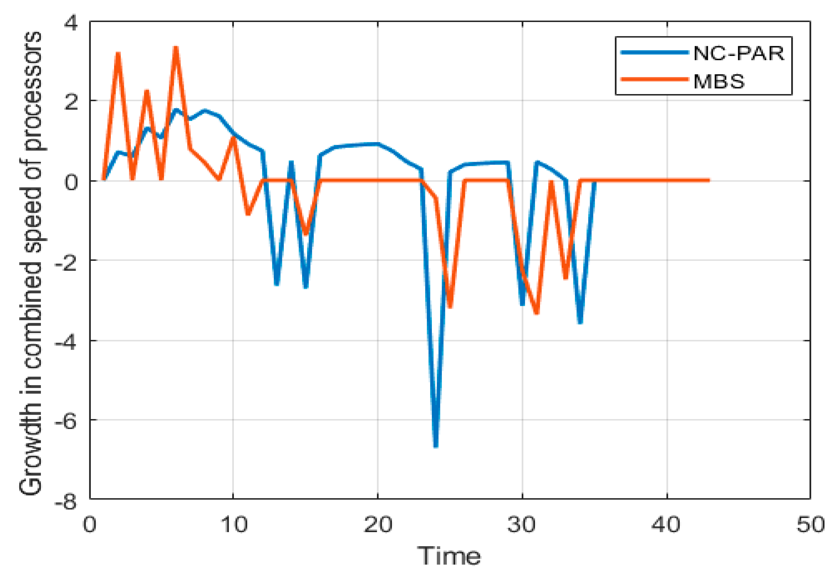
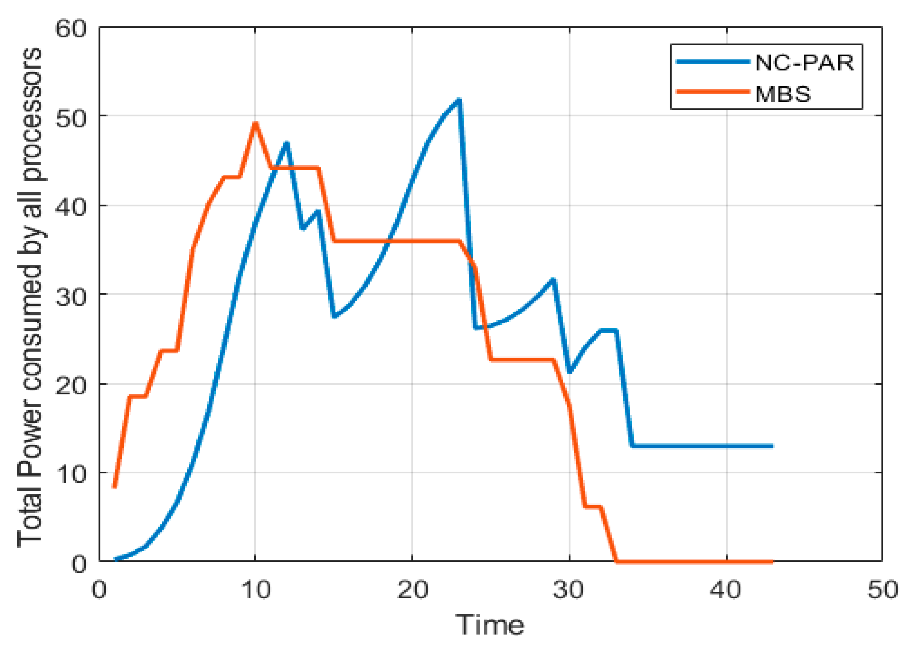
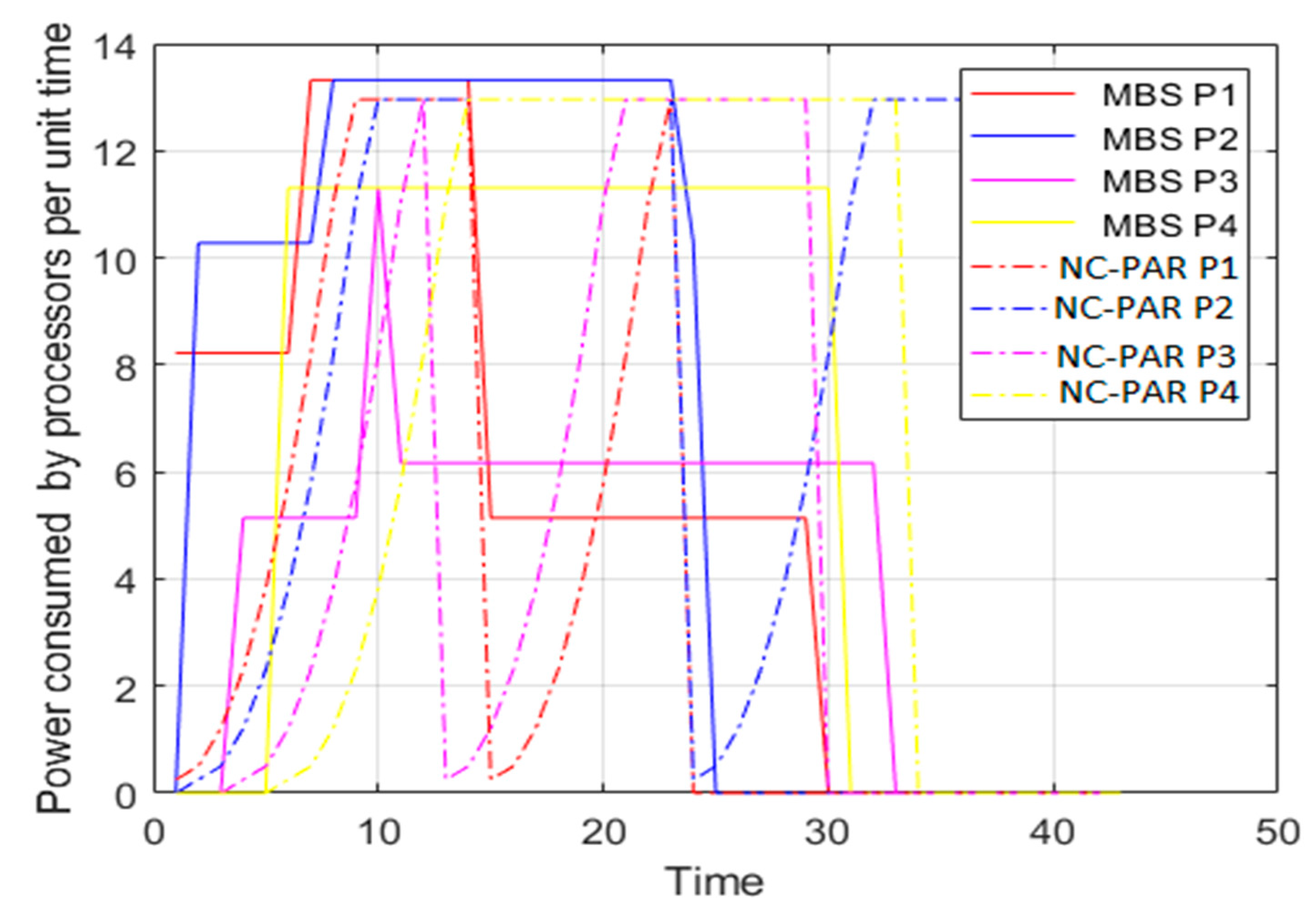
6. Illustrative Example

To observe the performance of MBS, a group of four processors and a set of seven jobs are considered. The best known result in the online non-clairvoyant scheduling algorithms is provided by the Azar et al. [40] in NC-PAR. NC-PAR is a super-constant lower bound on the competitive ratio of any deterministic algorithm even for fractional flow-time in the case of uniform densities. The processing of jobs using algorithms MBS and NC-PAR [40] is simulated and the results are stated in

Table 4. Job details and execution data using MBS and NC-PAR.

Job Details				MBS [This Paper]			NC-PAR [40]
Job	Size	Importance	Arrival Time	Completion Time	Response Time	Turnaround Time	Completion Time	Response Time	Turnaround Time
J1	35	8	1	14	0	13	14	0	13
J2	64	10	2	24	0	22	23	0	21
J3	15	5	4	10	0	6	12	0	8
J4	83	11	6	30	0	24	33	0	27
J5	45	5	7	29	0	22	29	6	22
J6	17	4	8	23	0	15	23	7	15
J7	56	6	10	32	0	22	43	14	33
Average Values				23.143	0	17.714	25.286	3.857	19.857

as well as in Figure 3, Figure 4, Figure 5, Figure 6, Figure 7, Figure 8, Figure 9, Figure 10 and Figure 11. The jobs arrived along with their importance but the size of jobs was computed on the completion of jobs. The response time (Rt) is the time interval between the starting time of execution and arrival time of a job. The turnaround time is the time duration between completion time and arrival time of a job. Most of the jobs using MBS have lesser turnaround time than using NC-PAR. The Rt of the jobs using MBS is better than NC-PAR. In Figure 3 and Figure 4, the allocation and execution sequence of jobs on four processors is depicted with the help of triangles and rectangles using NC-PAR and MBS, respectively. As per the Figure 3 and Figure 4, the importance of the jobs in NC-PAR increased with time where as in MBS the importance remains constant during the life time of the jobs. It is clearly evident from the Figure 3 and Figure 4 that on any processor using NC-PAR at a time only one job has been executed, whereas using MBS the processor has been shared by more than one job. The hardware specifications are mentioned in the

Table 5. Hardware specifications.

Simulation Parameters	Values
CPU	Intel(R) Core(TM) i5-4210U CPU @ 1.70 GHz
RAM	4.00 GB RAM
Hard Drive	1.0 TB
Operating System	Red Hat Linux 6.1
Kernel	Linux kernel version 2.2.12

.

Figure 5 and Figure 6 present the speed of different processors and combined speed of all processors with respect to time using MBS and NC-PAR, respectively. As per the graphs of Figure 5, the speed of a processor using MBS goes high initially but later it reduces and most of the time the speed of processors using MBS is constant, but when processors executes jobs using NC-PAR the speed of processors have heavy fluctuations, which shows that some extra energy may be needed for such frequent fluctuation in NC-PAR. The graphs of the Figure 6 shows that the combined speed of processors using NC-PAR increased and decreased linearly whereas using MBS it increased and decreased stepwise. The count of local maxima and minima in the speed growth graphs (Figure 7) of NC-PAR is more than MBS. Therefore, not only individual processor’s speed but also the combined speed of all the processors is reflecting the heavy fluctuation in NC-PAR and varying-constant mixed behaviour of MBS.

In this simulation analysis the traditional power function is used and the value of α is 2. The processors are having the maximum limit of speed which is considered 3.6. The value of $\Delta ={\left(3\alpha \right)}^{-1}$ is considered for the analysis. The power consumed is square of the speed, i.e., proportional to the speed this fact can be viewed by comparing the graphs of Figure 5 and Figure 9. Figure 8, shows that initially MBS consumed more power but power consumption decreased with respect to increase in time, whereas in case of NC-PAR there is no fix pattern, but power consumption is higher most of the time than in MBS.

The graphs of Figure 10 demonstrate the objective of the algorithm (important based flow time plus energy). It reveals that except one processor P1, all other processor have lesser objective value, when these processors executed jobs by using MBS than NC-PAR. The combined objective of all processor is given in the Figure 11, which strengthen the previous observation of Figure 10 (the objective values using MBS is lesser than using NC-PAR). It can be concluded from the different observations and the Figure 11, that the algorithm MBS performs better than NC-PAR.

7. Conclusions and Future Work

To date, the problem of ON-C scheduling algorithms with an objective to minimize the IbFt+E for multiprocessor setting is studied less extensively. A scheduling algorithm multiprocessor with bounded speed (MBS) is proposed, which uses importance-based/weighted round robin (WRR) for job selection. MBS extends the theoretical study of an ON-C multiprocessor DSS scheduling problem with an objective to minimize the IbFt+E using the bounded speed model, where every processor’s maximum speed using MBS is $\left(1+\raisebox{1ex}{$\Delta $}\!\left/ \!\raisebox{-1ex}{$3m$}\right.\right)\eta$ and using offline adversary Opt is $\eta$. The speed of any processor changes if there is a variation in the total importance of jobs on that processor. The competitiveness of MBS is $\left(\frac{9}{8}+\frac{3\Delta }{8}\right)·\left(1+{\left(1+\raisebox{1ex}{$\Delta $}\!\left/ \!\raisebox{-1ex}{$3m$}\right.\right)}^{\alpha }\right)=O\left(1\right)$ against an offline adversary, using the potential function analysis and traditional power function. The performance of MBS is compared with best known algorithm NC-PAR [40]. A set of jobs and processors are used to simulate the working of MBS and NC-PAR. The average turnaround and response time of jobs, when they are executed by using MBS is lesser than NC-PAR. The speed scaling strategy and power consumption in MBS is better than NC-PAR. For all processors at any time, MBS provides the lesser value of the sum of important-based flow time and energy consumed than NC-PAR. Competitiveness of NC-PAR is 3 for $\alpha =2$ and 3.5 for $\alpha =3$, whereas the value of competitive ratio c of MBS for $\Delta ={\left(3\alpha \right)}^{-1}$, $m=2$ and $\alpha =2$ is 2.442; for $\Delta ={\left(3\alpha \right)}^{-1}$, $m=2$ and $\alpha =3$ is 2.399; for $\Delta ={\left(3\alpha \right)}^{-1},$ $m>2$, $\alpha =2$ is $2.375<c<2.442$; for $\Delta ={\left(3\alpha \right)}^{-1}$, $m>2$, $\alpha =3$ is $2.333<c<2.399$. These results demonstrate that the scheduling algorithm MBS outperforms other algorithms. The competitive value of MBS is least to date. Before these outcomes, there were no results acknowledged for the multi-processor machines in the ON-C model with identified importance, even for unit importance jobs [40]. The further enhancement of this study will be to implement the MBS in real environment. One open problem is to achieve a reasonably less competitive algorithm than MBS. In this study, author considers non-migratory and sequential jobs and this work may be extended to find a scheduling for migratory and non-sequential jobs. Other factors (such as memory requirement) may also be considered for analysis in future extension.

References

1. Belady, C. In the Data Center, Power and Cooling Costs More Than the IT Equipment It Supports, Electronics Cooling Magazine. Available online: http://www.electronics-cooling.com/2007/02/in-the-data-center-power-and-cooling-costs-more-than-the-it-equipment-it-supports/ (accessed on 10 January 2020).
2. Chan, H.L.; Edmonds, J.; Lam, T.W.; Lee, L.K.; Marchetti-Spaccamela, A.; Prush, K. Non-clairvoyant speed scaling for flow and energy. Algorithmica 2011, 61, 507–517. [Google Scholar] [CrossRef] [Green Version]
3. Merritt, R. CPU Designers’ Debate Multi-Core Future, EE Times. 2 June 2008. Available online: http://www.eetimes.com/document.asp?doc_id=1167932 (accessed on 15 January 2020).
4. U.S. Environmental Protection Agency, EPA Report on Server and Data Center Energy Efficiency. Available online: https://www.energystar.gov/ia/partners/prod_development/downloads/EPA_Report_Exec_Summary_Final.pdf (accessed on 14 January 2020).
5. Singh, P.; Wolde-Gabriel, B. Executed-time Round Robin: EtRR an online non-clairvoyant scheduling on speed bounded processor with energy management. J. King Saud Univ. Comput. Inf. Sci. 2016, 29, 74–84. [Google Scholar] [CrossRef] [Green Version]
6. Bansal, N.; Chan, H.L.; Pruhs, K. Speed scaling with an arbitrary power function. In Proceedings of the Annual ACM-SIAM Symposium on Discrete Algorithms, New York, NY, USA, 4–6 January 2009; pp. 693–701. [Google Scholar]
7. Bansal, N.; Kimbrel, T.; Pruhs, K. Dynamic speed scaling to manage energy and temperature. J. ACM 2007, 54, 1–39. [Google Scholar] [CrossRef]
8. Singh, P.; Khan, B.; Vidyarthi, A.; Haes Alhelou, H.; Siano, P. Energy-aware online non-clairvoyant scheduling using speed scaling with arbitrary power function. Appl. Sci. 2019, 9, 1467. [Google Scholar] [CrossRef] [Green Version]
9. Lam, T.W.; Lee, L.K.; To, I.K.K.; Wong, P.W.H. Nonmigratory multiprocessor scheduling for response time and energy. IEEE Trans. Parallel Distrib. Syst. 2008, 19, 1–13. [Google Scholar]
10. Motwani, R.; Phillips, S.; Torng, E. Nonclairvoyant scheduling. Theor. Comput. Sci. 1994, 30, 17–47. [Google Scholar] [CrossRef] [Green Version]
11. Yao, F.; Demers, A.; Shenker, S. A scheduling model for reduced CPU energy. In Proceedings of the Annual Symposium on Foundations of Computer Science, Berkeley, CA, USA, 23–25 October 1995; pp. 374–382. [Google Scholar]
12. Koren, G.; Shasha, D. Dover: An optimal on-line scheduling algorithm for overloaded uniprocessor real-time systems. SIAM J. Comput. 1995, 24, 318–339. [Google Scholar] [CrossRef]
13. Leonardi, S.; Raz, D. Approximating total flow time on parallel machines. In Proceedings of the ACM Symposium on Theory of Computing, El Paso, TX, USA, 4–6 May 1997; pp. 110–119. [Google Scholar]
14. Kalyanasundaram, B.; Pruhs, K. Speed is as powerful as clairvoyant. J. ACM 2000, 47, 617–643. [Google Scholar] [CrossRef]
15. Edmonds, J. Scheduling in the dark. Theor. Comput. Sci. 2000, 235, 109–141. [Google Scholar] [CrossRef] [Green Version]
16. Kalyanasundaram, B.; Pruhs, K. Minimizing flow time nonclairvoyantly. J. ACM 2003, 50, 551–567. [Google Scholar] [CrossRef]
17. Becchetti, L.; Leonardi, S. Nonclairvoyant scheduling to minimize the total flow time on single and parallel machines. J. ACM 2004, 51, 517–539. [Google Scholar] [CrossRef] [Green Version]
18. Chekuri, C.; Goel, A.; Khanna, S.; Kumar, A. Multiprocessor scheduling to minimize flow time with epsilon resource augmentation. In Proceedings of the 36th Annual ACM Symposium on Theory of Computing, Chicago, IL, USA, 13–15 June 2004; pp. 363–372. [Google Scholar]
19. Chen, J.J.; Hsu, H.R.; Chuang, K.H.; Yang, C.L.; Pang, A.C.; Kuo, T.W. Multiprocessor energy efficient scheduling with task migration considerations. In Proceedings of the 16th Euromicro Conference on Real-Time Systems, Catania, Italy, 2 July 2004; pp. 101–108. [Google Scholar]
20. Albers, S.; Fujiwara, H. Energy-efficient algorithms for flow time minimization. ACM Trans. Algorithms 2007, 3, 49. [Google Scholar] [CrossRef]
21. Bansal, N.; Pruhs, K.; Stein, C. Speed scaling for weighted flow time. In Proceedings of the 18th Annual ACM-SIAM Symposium on Discrete Algorithms, New Orleans, LA, USA, 7–9 January 2007; pp. 805–813. [Google Scholar]
22. Lam, T.W.; Lee, L.K.; To, I.K.K.; Wong, P.W.H. Competitive non-migratory scheduling for flow time and energy. In Proceedings of the 20th ACM Symposium on Parallelism in Algorithms and Architectures, Munich, Germany, 14–16 June 2008; pp. 256–264. [Google Scholar]
23. Chadha, J.; Garg, N.; Kumar, A.; Muralidhara, V. A competitive algorithm for minimizing weighted flow time on unrelated processors with speed augmentation. In Proceedings of the Annual ACM Symposium on Theory of Computing, Bethesda, MD, USA, 31 May–2 June 2009; pp. 679–684. [Google Scholar]
24. Chan, S.H.; Lam, T.W.; Lee, L.K.; Liu, C.M.; Ting, H.F. Sleep management on multiple processors for energy and flow time. In Proceedings of the 38th International Colloquium on Automata, Languages and Programming, Zurich, Switzerland, 4–8 July 2011; pp. 219–231. [Google Scholar]
25. Albers, S.; Antoniadis, A.; Greiner, G. On multi-processor speed scaling with migration. In Proceedings of the 23rd Annual ACM Symposium on Parallelism in Algorithms and Architectures, San Jose, CA, USA, 4–6 June 2011; pp. 279–288. [Google Scholar]
26. Gupta, A.; Im, S.; Krishnaswamy, R.; Moseley, B.; Pruhs, K. Scheduling heterogeneous processors isn’t as easy as you think. In Proceedings of the 23rd Annual ACM-SIAM Symposium on Discrete Algorithms, Kyoto, Japan, 17–19 January 2012; pp. 1242–1253. [Google Scholar]
27. Chan, S.H.; Lam, T.W.; Lee, L.K.; Zhu, J. Nonclairvoyant sleep management and flow-time scheduling on multiple processors. In Proceedings of the 25th Annual ACM Symposium on Parallelism in Algorithms and Architectures, Montreal, QC, Canada, 23–25 July 2013; pp. 261–270. [Google Scholar]
28. Lawler, E.L.; Lenstra, J.K.; Kan, A.R.; Shmoys, D.B. Sequencing and Scheduling: Algorithms and Complexity. In Handbooks in Operations Research and Management Science; Elsevier: Amsterdam, The Netherlands, 1993; Volume 4, pp. 445–522. [Google Scholar]
29. Hall, H. Approximation algorithm for scheduling. In Approximation Algorithm for NP-Hard Problems; Hochbaum, D.S., Ed.; PWS Publishing Company: Boston, MA, USA, 1997; pp. 1–45. [Google Scholar]
30. Sgall, J. On-line scheduling. In Online Algorithms, The State of the Art; Fiat, A., Woeginger, G.J., Eds.; Springer: Berlin/Heidelberg, Germany, 1998; pp. 196–231. [Google Scholar]
31. Karger, D.; Stein, C.; Wein, J. Scheduling Algorithms, CRC Handbook of Theoretical Computer Science; CRC Press: Boca Raton, FL, USA, 1999. [Google Scholar]
32. Irani, S.; Pruhs, K. Algorithmic problems in power management. ACM SIGACT News 2005, 36, 63–76. [Google Scholar] [CrossRef] [Green Version]
33. Albers, S. Energy efficient algorithms. Commun. ACM 2010, 53, 86–96. [Google Scholar] [CrossRef] [Green Version]
34. Albers, S. Algorithms for dynamic speed scaling. In Proceedings of the 28th International Symposium of Theoretical Aspects of Computer Science, Dortmund, Germany, 10–12 March 2011; pp. 1–11. [Google Scholar]
35. Gupta, A.; Krishnaswamy, R.; Pruhs, K. Scalably scheduling power-heterogeneous processors. In Proceedings of the 37th International Colloquium on Automata, Languages and Programming, Bordeaux, France, 5–10 July 2010; pp. 312–323. [Google Scholar]
36. Fox, K.; Im, S.; Moseley, B. Energy efficient scheduling of parallelizable jobs. In Proceedings of the 24th Annual Symposium on Discrete Algorithms, New Orleans, LA, USA, 6–8 January 2013; pp. 948–957. [Google Scholar]
37. Thang, N.K. Lagrangian duality in online scheduling with resource augmentation and speed scaling. In Proceedings of the 21st European Symposium on Algorithms, Sophia Antipolis, France, 2–4 September 2013; pp. 755–766. [Google Scholar]
38. Im, S.; Kulkarni, J.; Munagala, K.; Pruhs, K. SelfishMigrate: A scalable algorithm for non-clairvoyantly scheduling heterogeneous processors. In Proceedings of the 55th IEEE Annual Symposium on Foundations of Computer Science, Philadelphia, PA, USA, 18–21 October 2014; pp. 531–540. [Google Scholar]
39. Bell, P.C.; Wong, P.W.H. Multiprocessor speed scaling for jobs with arbitrary sizes and deadlines. J. Comb. Optim. 2015, 29, 739–749. [Google Scholar] [CrossRef] [Green Version]
40. Azar, Y.; Devanue, N.R.; Huang, Z.; Panighari, D. Speed scaling in the non-clairvoyant model. In Proceedings of the 27th Annual ACM Symposium on Parallelism in Algorithms and Architectures, Portland, OR, USA, 13–15 June 2015; pp. 133–142. [Google Scholar]
Figure 1. Performance and speed curve.
Applsci 10 02459 g001
Figure 2. Flow chart of the MBS scheduling algorithm.
Applsci 10 02459 g002
Figure 3. Scheduling of jobs using NC-PAR.
Applsci 10 02459 g003
Figure 4. Scheduling of jobs using MBS.
Applsci 10 02459 g004
Figure 5. Speed of processors using MBS and NC-PAR.
Applsci 10 02459 g005
Figure 6. Combined speed of all processors using MBS and NC-PAR.
Applsci 10 02459 g006
Figure 7. Growth of combined speed of all processors using MBS and NC-PAR.
Applsci 10 02459 g007
Figure 8. Total power consumed by all processors using MBS and NC-PAR.
Applsci 10 02459 g008
Figure 9. Power consumed by processors using MBS and NC-PAR.
Applsci 10 02459 g009
Figure 10. Importance-based flow time + energy consumed using MBS and NC-PAR.
Applsci 10 02459 g010
Figure 11. Total importance-based flow time + energy consumed using MBS and NC-PAR.
Applsci 10 02459 g011