AMBIQUAL: Towards a Quality Metric for Headphone Rendered Compressed Ambisonic Spatial Audio
by

Miroslaw Narbutt
1, 
Jan Skoglund
2,
Andrew Allen
2,
Michael Chinen
2,
Dan Barry
3 and
Andrew Hines
3,* 1
School of Electrical and Electronic Engineering, Technological University Dublin, D08 NF82 Dublin 8, Ireland
2
Chrome Media, Google, San Francisco, CA 94105, USA
3
School of Computer Science, University College Dublin, D04 N2E5 Dublin 4, Ireland
*
Author to whom correspondence should be addressed.
Appl. Sci. 2020, 10(9), 3188; https://doi.org/10.3390/app10093188
Submission received: 4 April 2020
/
Revised: 29 April 2020
/
Accepted: 30 April 2020
/
Published: 3 May 2020
Abstract
:Featured Application
Streaming spatial audio for immersive audio and virtual reality applications will require compression algorithms that maintain the localization accuracy and irrationality attributes of sound sources as well as a high-fidelity quality of experience. Models to evaluate quality will be important for media content streaming application such as YouTube as well as VR gaming and other immersive multimedia experiences.
Abstract
Spatial audio is essential for creating a sense of immersion in virtual environments. Efficient encoding methods are required to deliver spatial audio over networks without compromising Quality of Service (QoS). Streaming service providers such as YouTube typically transcode content into various bit rates and need a perceptually relevant audio quality metric to monitor users’ perceived quality and spatial localization accuracy. The aim of the paper is two-fold. First, it is to investigate the effect of Opus codec compression on the quality of spatial audio as perceived by listeners using subjective listening tests. Secondly, it is to introduce AMBIQUAL, a full reference objective metric for spatial audio quality, which derives both listening quality and localization accuracy metrics directly from the B-format Ambisonic audio. We compare AMBIQUAL quality predictions with subjective quality assessments across a variety of audio samples which have been compressed using the Opus 1.2 codec at various bit rates. Listening quality and localization accuracy of first and third-order Ambisonics were evaluated. Several fixed and dynamic audio sources (single and multiple) were used to evaluate localization accuracy. Results show good correlation regarding listening quality and localization accuracy between objective quality scores using AMBIQUAL and subjective scores obtained during listening tests.
Keywords:
virtual reality; spatial audio; Ambisonics; audio coding; audio compression; Opus codec; MUSHRA; audio quality; QoE1. Introduction
To create an immersive virtual reality experience both graphics and spatial audio need to be of high quality and synchronized to the user’s head movements in real time. In addition, audio sources must be accurately positioned such that they are localized at the correct azimuth and elevation. The most popular spatial audio format, known as Ambisonics B-format, was developed in the 1970s [1] and has been adopted by Google as the preferred audio format for Google VR and YouTube [2]. Facebook also implements Ambisonics in the Oculus headset. In contrast to existing channel-based methods such as stereo, 5.1, or 7.1 surround sound, Ambisonics B-format does not encode loudspeaker information. Instead it encodes the whole spherical soundfield around the listener’s head using spherical harmonics. A key advantage is that it is independent of any specific loudspeaker configuration. Ambisonics audio may be decoded to any loudspeaker layout and any number of loudspeakers, including a pair of headphones which will be the focus of our study.
Efficient encoding techniques are required for spatial audio streaming over networks. Such techniques should be capable of compressing audio content without affecting quality of experience. Objective audio quality metrics to predict quality and spatial localization accuracy of compressed spatial audio are required by many streaming services. Our work focuses on compressed spatial audio delivery for YouTube 360 videos which are typically consumed on VR headsets in which audio is delivered over headphones. As such, the experiments presented do not deal with Ambisonic audio delivered over loudspeakers.
Spatial audio is a broad and active research topic. Capturing, storing, transporting and delivering high-fidelity spatial audio poses many challenges that are out of scope for this work. This paper presents AMBIQUAL, a full reference objective audio quality metric designed to estimate the robustness of Ambisonic audio to compression in terms of perceived quality and localization accuracy. More specifically, we compare AMBIQUAL quality predictions with subjective quality assessments across a variety of natural and synthetic audio samples which have been compressed using the Opus 1.2 codec at various bit rates. We focus on the Opus 1.2 codec in this paper given its prevalent use in YouTube but the methodology described here can be applied to any spatial audio codec.
The AMBIQUAL model is built on previous research described in [3,4]. In [3] we investigated, via subjective audio listening tests, the effect of compression on the listening quality and localization accuracy of single point source spatial audio sources. In [5] the impact of multi-directional audio-visual fusion on speech quality and intelligibility was explored. In [4] we proposed a full reference objective quality model for Ambisonic spatial audio, and we showed a good correlation between objective quality scores calculated with AMBIQUAL algorithm and subjective scores gathered during listening tests.
This paper expands on the subjective audio listening tests presented in [3] from single point to multiple point audio sources. More complex sound scenes require further investigation and will be the topic of future work. It proposes adaptations to the AMBIQUAL algorithm where localization accuracy is calculated as a weighted product (rather than weighted sum) of similarity between reference and test Ambisonic directional channels. Lastly, it uses subjective quality scores gathered during listening tests to validate the new AMBIQUAL algorithm.
Section 2 presents an introduction to Ambisonics, the Opus compression scheme for spatial audio, and the subjective experimental methodology used to evaluate and label the spatial audio samples for quality and localization accuracy. Section 3 describes the preparation of experimental samples and the subjective testing methodology employed. Section 4 presents the AMBIQUAL model for predicting the effect of compression of Ambisonic audio quality and localization accuracy along with the experimental work to optimize the model. Section 5 presents two validation experiments: one using 206 points of a full sphere to confirm localization predictions and a second to evaluate the model using data from unseen subjectively labeled data. Section 6 discusses the results and presents possible future work.
2. Background
2.1. Ambisonics
Ambisonics is a 3D spatial audio format which allows sound sources to be placed above, below and behind the listener in addition to the horizontal plane supported by 2D audio formats. The format uses spherical harmonics to encode the audio such that the sources can be mapped to any location on the inner surface of a sphere, the center of which is the listener position. More specifically, Ambisonics B-format is independent of loudspeaker layout and the number of loudspeakers used. As a result, Ambisonics is a popular audio format for VR and AR use cases given that it allows full rotation of the soundfield in three dimensions [6]. Most VR headset applications require audio to be presented binaurally and respond to head movement in real time, making Ambisonics an ideal choice.
An infinite number of spherical harmonics would be required to achieve perfect localization within the Ambisonics soundfield but this is not practical due to the amount of data required. As a result, a smaller number of spherical harmonics is used. The most popular format today, known as first-order Ambisonics (FOA), uses 4 spherical harmonics denoted as W, X, Y and Z. The W channel represents an omnidirectional gain and channels X, Y and Z respectively represent front-back, left-right, and up-down directions within a sphere. The B-format representation can be extended from FOA to second and third-order Ambisonics (SOA and 3OA) to get higher localization accuracy. Second-order and third-order Ambisonics contain 9 and 16 channels, respectively. It was found in [7] that third-order Ambisonics (3OA) gives a significantly better Quality of Experience (QoE). This is further supported in [3]. In [8], subjective testing shows that localization accuracy decreases monotonically as a function of both order number and codec bit rate. Figure 1 shows the spherical harmonics associated with first, second and third-order Ambisonics. As illustrated, the second order encapsulates the 4 harmonics comprising the first order. Similarly, the third order encapsulates the 9 harmonics comprising the first and second orders combined. As a result, it should be noted that the number of channels increases according to where n is the order.
Using higher-order Ambisonics (HOA) results in better localization accuracy and better listening quality [3] but the large amount of data to be processed requires higher transmission bandwidth and processing power. To facilitate this, efficient codecs are required to compress spatial audio without compromising QoE.
2.2. Opus 1.2 Codec with Channel Mapping
The Opus codec is an open-source audio codec intended for real-time VoIP and videoconferencing applications and for streaming audio over the Internet [9]. Opus can handle very low bitrate narrowband speech as well as very high-quality multi-channel music. It has been adopted by applications such as Skype, Google Hangouts and YouTube. It is included in the WebRTC API as “mandatory to implement” [10].
Ambisonic spatial audio can be encapsulated in Ogg format by encoding it with the Opus codec and setting the channel mapping family value to 2 or 3. For FOA, it is recommended to use channel mapping 2, which encodes each Ambisonic channel independently. For HOA, channel mapping 3 provides a more efficient encoding. The channel mapping family 2 allows for so-called mixed-order Ambisonic representations where only a subset of the full Ambisonic order number of channels is required [11].
This work investigates, via MUSHRA subjective listening tests, the effect of Opus codec compression using channel mapping family 2, on the listening quality and localization accuracy of spatial audio as perceived by listeners. The results of MUSHRA subjective listening tests have been used to validate and optimize a full reference objective spatial audio quality metric described in Section 4 of this paper.
2.3. Subjective and Objective Methods of Assessing Audio Quality
Subjective methods of assessing audio quality and localization accuracy are time consuming and resource intensive. There have been various recent studies in the area, e.g., [12,13] including some of particular relevance [8,14] but objective measures are needed for large scale complex streaming services. Objective methods using computer models to assist in rapidly predicting speech and audio quality have been developed. Objective metrics exist for speech (e.g., POLQA [15,16]) and audio quality (e.g., PEAQ [17,18]) but no objective metrics are agreed upon for compressed spatial audio quality evaluation. Although early work to extending PEAQ to spatial audio was published [19] it did not yield a recommendation. Audio quality can be evaluated using subjective testing in the absence of objective assessment methods. Accepted subjective testing methods for assessing speech and audio quality include, ITU Rec. ITU-T P.800 for speech [20], ITU-R Rec. BS.1534-3 [21] and BS.1116-3 [22], and the recently published P.1310 for Spatial audio meetings quality [23].
3. Subjective Listening Tests Using the MUSHRA Methodology
3.1. Method
To demonstrate the impact of spatial audio compression on perceived audio quality, a set of subjective listening tests were carried out using a double-blind multi-stimulus test method with a hidden reference and hidden anchor (MUSHRA) following the ITU-R BS.1534-3 Recommendation. During the listening tests, subjects were presented with a labeled reference and several unlabeled test samples. The subjects were asked to rate different samples for a set of encoding conditions such as Ambisonic order and encoding bit rates. They were asked to assign quality ratings from 0 to 100 to the unlabeled test samples using a numerical continuous scale in five intervals: bad (0–20), poor (20–40), fair (40–60), good (60–80), and excellent (80–100).
3.2. Testing Platform and Testing Environment
The WebMUSHRA platform [24] was used for conducting the listening tests. It is an open-source web-based application which implements the ITU-R BS.1534-2 Recommendation.
The WebMushra Graphical User Interface is shown in Figure 2. For each example, the listener is presented with buttons to play back the reference signal along with 5 different encoded versions of the same signal, one of which is a hidden reference. The test subjects can play back the examples as many times as they wish. For each of the 5 encoded versions, the listener is asked to rate the localization accuracy on a scale from 0–100, using a slider beneath each play button. The listeners can also select and loop a segment of the audio if they wish.
The subjective listening tests were carried out in controlled environments within Technological University Dublin (TUD) and Trinity College Dublin (TCD). A small number of tests were conducted remotely by experienced listeners in controlled environments. For the tests carried out in TUD and TCD, the WebMUSHRA test system was set up on a laptop with a set of Audio-Technica ATH-M70x headphones which exhibit a flat frequency response spanning the range 5 Hz to 40 kHz. For each test subject, the resulting quality scores were examined following the ITU MUSHRA recommendation.
3.3. Testing Procedure
Before the listening tests were conducted, assessors undertook a training session which allowed them to become familiar with the Graphical User Interface and the testing procedures and evaluation method. This training session ensures reliable results.
During the actual listening tests, the assessors were asked to rate test audio sources in regards to two aspects: listening quality and localization accuracy. They were defined as follows:
Listening quality:
- distortion of the audio signal as compared to the reference
- undesired sounds that add artefacts to the audio clips under test
Localization accuracy:
- how accurately test audio sources are positioned as compared to the reference
- how well test audio sources track movements of the reference
3.4. Experiment 1-Single Point Audio Sources
Both listening quality and localization accuracy were evaluated using single point audio sources. Twenty-one assessors (20 male and 1 female) took part in the listening tests. The average age was 32 and the age range was between 20 and 53. Among assessors, there were 9 experienced listeners (professional audio engineers and academics with prior experience of similar tests) 12 semi-experienced listeners (post-graduate students in TUD and TCD). Following the ITU-T recommendation, subjects who gave the hidden reference a score of less than 90 for more than 15% of the test items were excluded. Results of three outliers were excluded. The AmbiX decoder [25] with the SADIE II database [26] was used to render the Ambisonic audio for binaural subjective presentation.
3.4.1. Content
Five audio samples were used with durations of 7 to 15 s. Various musical sounds were selected from CDs and the EBU music database [27]. The content was chosen as for the compression challenges they pose to codecs and the samples have previously been evaluated for stereo quality [28]. Additionally, one audio sample (pinkReverb) was synthetically generated. For reverb samples, a simple mono to mono impulse response convolution was initially applied to the original mono reference signal. All clips had a sampling frequency of 48 kHz (one example was re-sampled from 44.1 kHz) and were recorded in stereo format. Details of the audio samples used in experiment 1 can be found in Table 1.
3.4.2. Localization
The FOA and 3OA mono audio samples were used to create single point audio sources with various fixed and dynamic localizations as shown in Figure 3.
3.4.3. Conditions
Ambisonic B-format content audio signals were encoded using the Opus 1.2 codec with channel mapping family 2 implementation [11] at a variety of bit rates to produce a range of conditions. These signals were then rendered to a binaural format for headphone presentation using a generic head related transfer function (HRTF). For FOA examples, a Neumann KU 100 binaural dummy head (SADIE subject 2) with a cube layout was used. For 3OA examples, the same KU 100 binaural dummy head using a 26-point Lebedev Quadrature layout was used with the angles presented in Table 2. The layout and post-processing procedure followed for both 1st and 3rd order HRTFs are described on the SADIE project website (https://www.york.ac.uk/sadie-project/GoogleVRSADIE.html). Head symmetry optimization (assuming the ears are reverse-identical filters) was applied by inverting the L/R HRTFs around the head to save on computation. Negligible differences were found between the original HRTFs and these symmetrical versions using this technique as outlined in [29].
Rendered audio content signals (i.e., test samples) were created for a range of conditions. The original uncompressed audio, 3OA, serves as both the “Reference” condition and the hidden reference for this MUSHRA test. Third-order Ambisonics (3OA) audio encoded with 512 and 256 kbps serve as conditions 3OA512 and 3OA256, respectively. First-order Ambisonics audio (FOA) encoded at 128 and 64 kbps serve as conditions FOA128 and FOA64, respectively. Finally, condition FOA32 was used as the hidden anchor for testing and represents first-order Ambisonic audio encoded at 32 kbps. Details of encoding schemes and bit rates used in Experiment 1 can be found in Table 3.
3.4.4. Results
Aggregated subjective listening quality scores by encoding scheme (with mean values and 95% confidence intervals) are shown in Section 4.6. Aggregated subjective localization accuracy scores are also shown in Section 4.6. The aggregated scores are estimated here as the average MUSHRA scores obtained for all nine audio test samples. Single point sources with fixed localizations are denoted in this paper with suffix “F”. Sources moving vertically (i.e., dynamic elevation) are denoted with suffix “El” and moving horizontally (i.e., dynamic azimuth) are denoted with suffix “Az”.
Full details and analysis of this experiment are presented in [3]. In summary, listening quality and localization accuracy are greatly impacted by compression using the Opus 1.2 codec. This is confirmed by the listening tests. The quality of experience depends largely on the channel bit rate used. Listening quality was deemed to be “good” for conditions 3OA512 and FOA128. Localization was deemed to “excellent” for condition 3OA512. Lower bit rates have detrimental effects on listening quality and localization accuracy. It was observed that with bit rates of 16 kbps per channel (used by 3OA256 encoding scheme) 3OA no longer outperforms FOA.
3.5. Experiment 2-Multiple Point Audio Sources
The results from experiment 1 showed that quality could be predicted from analysis of ACN 0 (the omnidirectional channel) but as expected, that localization accuracy was influenced by the subsequent channels. In order to further investigate localization accuracy, a second MUSHRA test was designed using multiple point sources. In contrast to experiment 1 where single point audio sources were used, this time only localization accuracy was evaluated.
A different cohort of listeners took part in experiment 2, with some overlap with the listeners from experiment 1. In total 20 participants performed the test and 13 results were taken into account (7 listeners gave the hidden reference a score of less than 90 twice or more times). The participants included 5 experienced listeners and 8 semi-experienced listeners with an average age of 33 ranging from 21 to 50. The exclusion of inexperienced listeners who failed to identify the reference after initial training reinforced the importance of using experienced listeners in spatial audio testing.
3.5.1. Content
For the second experiment six audio samples have been originated from the EBU music database, one (pinkReverb) was synthetically generated, and one (babble noise) was taken from the TCD-VoIP dataset [30]. All audio clips were sampled at 48 kHz. They were converted to mono format and then encoded to FOA and 3OA formats with a variety of localizations. Details of audio samples used in experiment 2 can be found in Table 4.
3.5.2. Localization
The FOA and 3OA audio samples were used to create multi-point audio sources with various localizations (one source with fixed localization and one moving vertically or horizontally) as shown in Figure 4.
3.5.3. Conditions
As in experiment 1, the Ambisonic audio samples were encoded using Opus 1.2 codec, channel mapping family 2 at various bit rates to produce a range of conditions. They were then rendered to a binaural format for presentation. Conditions under the tests included: “Reference”, 3rd-order Ambisonics audio: 3OA512, 3OA384, 3OA256 and first-order Ambisonic audio: FOA128, FOA96, FOA64, FOA32. The last condition, encoded at 32kbps (8kbps per channel), was used as the hidden anchor.
Details of encoding schemes and bit rates used in Experiment 2 can be found in Table 5.
3.5.4. Results
Aggregated MUSHRA scores by encoding scheme (with mean values and 95% confidence intervals) are shown in Section 4.6.
Multiple point audio sources are denoted in this paper as concatenations of fixed and dynamic audio source labels. Audio sources with fixed localizations are denoted with suffix “F”. Sources moving vertically (i.e., dynamic elevation) are denoted with suffix “El” and moving horizontally (i.e., dynamic azimuth) are denoted with suffix “Az”. For example, an audio source denoted as “pianoFxylEl” represents multiple point audio source with one piano sound source at fixed location and one xylophone sound source moving vertically (i.e., with dynamic elevation).
Experiment 2 confirmed that both Ambisonics order and audio channel compression affects localization accuracy of multiple point audio sources. All third-order Ambisonics above 16 kbps per channel (i.e., 3OA512, 30A384, 3OA256) and one first-order Ambisonics with 32 kbps bit rate per channel (i.e., FOA128) were rated “excellent” or “good” in regards to localization accuracy.
The results of these experiments have been used to optimize (experiment 1) and validate (experiment 2) a new objective quality model for spatial audio described in next sections of this paper.
4. An Objective Model for Coded Spatial Audio QoE Prediction
To assess the effect of spatial audio compression on listening quality and localization accuracy, we propose a new method. AMBIQUAL is a dedicated spatial audio quality assessment method adapted from the ViSQOLAudio algorithm [18]. The method we present below extends an earlier prototype described in [4].
4.1. ViSQOLAudio
The Virtual Speech Quality Objective Listener Audio (VISQOLAudio) is a signal-based full reference quality metric that uses a spectro-temporal measure of similarity between a reference and a test audio signal [18]. The assessment method has three major processing stages: pre-processing, time-alignment, and similarity assessment. In the pre-processing stage the test signal is scaled to match the reference signal’s sound pressure level. In the time-alignment stage, two spectrogram representations of the reference and test signals are created using a Gammatonegram filter bank (with 32 critical frequency bands uniformly spaced on the Equivalent Rectangular Bandwidth scale between the lowest central frequency of 50 Hz and highest central frequency of 14,064 Hz respectively). Then the reference spectrogram is segmented into patches 480 ms long (30 frames, each 16 ms) and each reference patch is aligned with the corresponding test patch. Spectrogram patches are treated as images and a metric called Neurogram Similarity Index Measure (NSIM) [31] is used for time-alignment and similarity assessment. This NSIM metric is a simplified version of the Structural Similarity Index Measure (SSIM) which was developed to assess JPEG images quality relative to reference uncompressed versions of the same images [32]. In this work, the resulting similarity scores (i.e., NSIM scores between 0 and 1) are calculated for each spectrogram patch separately and averaged over the patches to yield the overall similarity metric for the test signal. Figure 5 shows spectrogram patches of the reference and test signals, similarity map, and corresponding NSIM scores.
4.2. AMBIQUAL Design Considerations
Humans use the differences in the acoustic signals reaching the two ears to localize sound sources. The work by Rayleigh [34] concluded that there were two cues for determining location: Interaural Time Difference (ITD), which provides information for low-frequency stimuli, and the Interaural Level Difference (ILD), which provides location information at high frequencies. According to Rayleigh’s duplex theory the ITD is used at low frequencies (below 1500 Hz), where phase difference is unambiguous, and the ILD is used at high frequencies, where the “head shadow” effect results in large amplitude differences. It has also been shown in recent research that envelope as well as fine structure cues can be used by the auditory system to capture ITD. This was shown to be useful in localization models for binaural signals [35]. Observations from lateralization experiments lead to a conclusion that ITD is the cue used to locate any sound with low frequencies or any high-frequency complex sound with a low-frequency repetition in the time-domain waveform [36].
Sounds not arising directly from in front (or behind) arrive earlier at one ear than at the other, creating an ITD. As shown in Figure 6, the sound travels a shorter distance to the right ear than to the left ear; this yields an ITD. For wavelengths roughly equal to, or shorter than, the diameter of the head, a shadowing effect is produced at the ear further from the source, creating an ILD. It is worth mentioning that the ITD for any frequency is theoretically the same for all frequencies for a particular stimulus location, whereas the Interaural Phase Difference (IPD) will vary according to the frequency of the stimulus [36].
The idea behind the AMBIQUAL algorithm is to use signal information which is embedded in Ambisonic audio channels to calculate QoE as perceived by listeners. The aim is to predict a composite QoE degradation resulting from compression for a given spatial audio signal. It does not consider other factors, e.g., head listening direction with respect to source cues or the influence of the HRTF used in rendering the binaural signal. Unlike existing methods that estimate the direction of audio sources by analysis of binaurally rendered signals [37] or energetic analysis [38,39] the proposed AMBIQUAL algorithm operates directly on the B-format Ambisonic audio channels to derive Listening Quality and Localization Accuracy metrics.
As with ViSQOLAudio, the AMBIQUAL approach uses a time-frequency representation to measure the similarity between a reference and a test audio signal. This time, however, a spectrogram of phase angles rather than magnitudes is used for the signal similarity comparisons. After the pre-processing stage, when the test signal is scaled to match the reference signal’s sound pressure level, two “phaseogram” representations of the reference and test signals are created. Phaseograms are computed using a 2048-point STFT (with 1536-point Hamming window, 50% overlap). In order to match gammatone frequency bands derived from Equivalent Rectangular Bandwidth scale (i.e., between the lowest central frequency of 50 Hz and highest central frequency of 14,064 Hz) the number of frequency bins is reduced to first 640 (i.e., from 23 Hz to 15,000 Hz). Like before, the reference phaseogram is segmented into patches 480 ms long (30 frames, each 16 ms) and each reference patch is aligned with the corresponding test patch. The similarity between reference and test phaseogram patches are computed frame by frame taking into account all 640 frequency bins. Resulting NSIM scores are averaged across 32 frequency bands corresponding to 32 critical gammatonegram frequency bands. Then, the similarity scores are calculated for each patch separately and averaged over the patches to yield the resulting similarity NSIM score for the test signal.
A simple example with phaseograms derived from one directional Ambisonic channel (ACN = 1) illustrate that NSIM scores decreased as the test signals moved away from the reference. Figure 7 and Figure 8 show 640-bin phaseograms, 32-band similarity maps, and corresponding similarity scores (NSIMs) calculated for two test signals, each pure sine wave tones of 100 Hz, localized in two different positions in relation to the reference. When the reference signal is localized at {Azimuth = 60, Elevation = 60}, and test signals localized at {Azimuth = 50, Elevation = 60} and {Azimuth = 10, Elevation = 60}, the resulting NSIM scores are 0.944 and 0.918 respectively (as shown in Figure 7 and Figure 8)
4.3. Deriving Listening Quality from B-Format Ambisonic Audio
Within the Ambisonics B-format, the omnidirectional channel, W, contains contributions from all other directional channels. As such, we can assume it to be a good representation of all channels for the purposes of measuring encoding artefacts (except for localization differences). As a result, listening quality, , is computed by applying the AMBIQUAL algorithm to the phaseograms of the reference, r and test, t, to channel , i.e.,
The resulting is a bounded similarity score between 0 and 1 where 1 is a perfect match.
4.4. Deriving Localization Accuracy from B-Format Ambisonic Audio
Localization accuracy, (), can be computed as a weighted product of similarity between reference, r, and test, t, Ambisonic channels as follows:
where N is the number of Ambisonic channels, is the phaseogram similarity between k-th reference Ambisonic channel and k-th test Ambisonic channel as measured by the modified ViSQOLAudio algorithm and is an exponent (weighting factor) applied to the k-th phaseogram’s similarity measure. Due to the symmetry of Ambisonic channels, it is possible to reduce the number of exponents as follows:
Exponents related to horizontal channels:
- ;
- ;
- ,
exponents related to mixed-orientation channels:
- ;
- ;
- ,
and exponents related to vertical channels:
- ;
- ;
- ,
Resulting is a bounded similarity score between 0 and 1 where 1 is a perfect match.
4.5. Compensating for Empty or Non-Existing Channels
The B-format Ambisonic audio can contain empty (i.e., zero-padded channels) especially if scenarios where there is no background ambient sound as the sources were synthetically generated (see Figure 9). There are also scenarios where the test file is a lower order than the reference, e.g., a FOA Ambisonic audio test (containing 4-channels) is compared to a 3OA reference (containing 16-channels). In this case the algorithm must reconcile the fact that 12 channels are not present in the test. Empty or non-existent channels would impact the overall similarity computation by AMBIQUAL. When the reference and the test channels are both empty, the algorithm sets the similarity NSIM score to 1 as the test channel is identical to the reference. However, when a reference channel contains data and the test signal is empty the algorithm computes an invalid NSIM score (NaN) due to zeros in the denominator. Due to the product computation for localization accuracy in eqn (2), this would result in an invalid overall similarity computation.
To mitigate the effect of empty or non-existing channels, all invalid (NaN) are substituted with a minimum threshold value before applying it to Equation (2). The optimal value for this threshold, , was experimentally obtained using the experiment 1 data.
The values of , , , , , , , and were chosen experimentally to maximize correlation (both Spearman and Pearson) between AMBIQUAL results and MUSHRA scores obtained during experiment 1 (i.e., listening tests with single point audio sources). A wide range of values were tested. The values presented provided the best results. The results were robust if the relative relationships were similar. The general trend can be described as follows: the first-order horizontal channels were weighted more than the vertical channel but only by a small amount (4%). The second and third-order vertical channel weightings are a magnitude less than the first-order channel weightings. The horizontal second and third-order weightings were a further magnitude lower and the mixed-orientation channel weights a further magnitude less.
Both listening quality and localization accuracy were evaluated with various combinations of , , , , , , , , and and were compared to subjective MUSHRA scores collected from experiment 1. Pearson and Spearman correlation were calculated for all the test results except for comparing the reference to itself. This would result in higher ranking scores due to perfect matches for the objective model.
Using weighting factors’ values shown in Figure 10 and set to 0.1 resulted with a good correlation (Pearson = 0.922, Spearman = 0.919) between AMBIQUAL results and subjective MUSHRA scores.
4.6. AMBIQUAL Results
4.6.1. Listening Quality
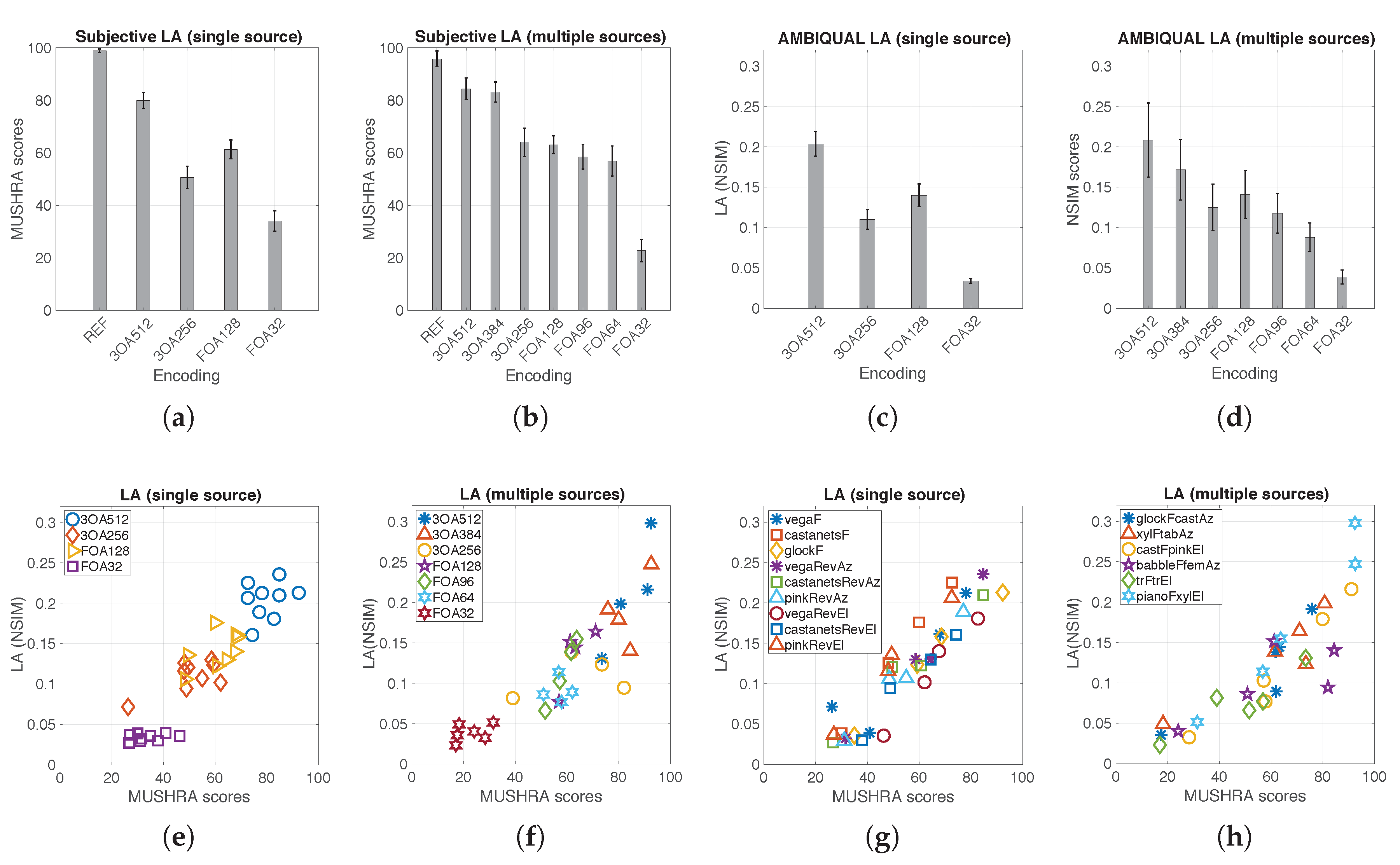
As described in Section 4.3, is computed by applying a modified version of the ViSQOLAudio algorithm to the omnidirectional Ambisonics channel as per eqn (1). Aggregated AMBIQUAL listening quality predictions by encoding scheme, with mean values and 95% confidence intervals, are presented in Figure 11a.
Subjective MUSHRA quality scores are compared to objective AMBIQUAL quality predictions in Figure 11c (by encoding scheme) and Figure 11d (by content type). Results show a good correlation (Pearson = 0.899; Spearman = 0.816) between subjective scores and objective predictions. The results by condition demonstrate condition clustering and the results by content type confirm that the model is not biased by content.
4.6.2. Localization Accuracy
As described in Section 4.4, localization accuracy is computed as a weighted product of similarity between Ambisonics reference and test directional channels as per eqn. (2). Objective model predictions of localization accuracy are presented in Figure 12c. Here, the aggregated mean values of the localization accuracy scores are shown for the 4 encoding schemes. The 95% confidence intervals are also shown.
AMBIQUAL localization accuracy scores are compared with subjective MUSHRA scores in Figure 12e (per condition) and Figure 12g (per sample content). Results show good correlation between objective AMBIQUAL and subjective MUSHRA quality scores (Pearson’s corr = 0.922, Spearman’s corr = 0.919). Again, as with the quality test, the condition and not the sample content is the dominating factor influencing localization accuracy.
5. Validation Experiments
5.1. Full Sphere Localization Accuracy Prediction
Building on the initial exploration in [4], a dataset of one second duration, pink noise audio signals, sampled at 48kHz were synthetically generated. Third-order Ambisonics B-format was used to render the reference audio sources to 22 fixed locations, evenly distributed over a quarter of a sphere. The test Ambisonic audio signals were rendered at 206 fixed locations evenly distributed on the whole sphere (i.e., with 30 horizontal and 10 vertical steps as illustrated in Figure 13). Localization accuracy was computed for each combination of the reference and test audio sources.
Figure 13 presents an example of results for one reference signal, marked in red where the test signal accuracy of predictions are in grayscale, descending light to dark. In this example, the source was anchored at 60 azimuth and 60 elevation. As can be seen, the test localization accuracy decreases as it gets further from the reference source. This is indicated by the grey dots getting darker as the test signal location gets further from the reference.
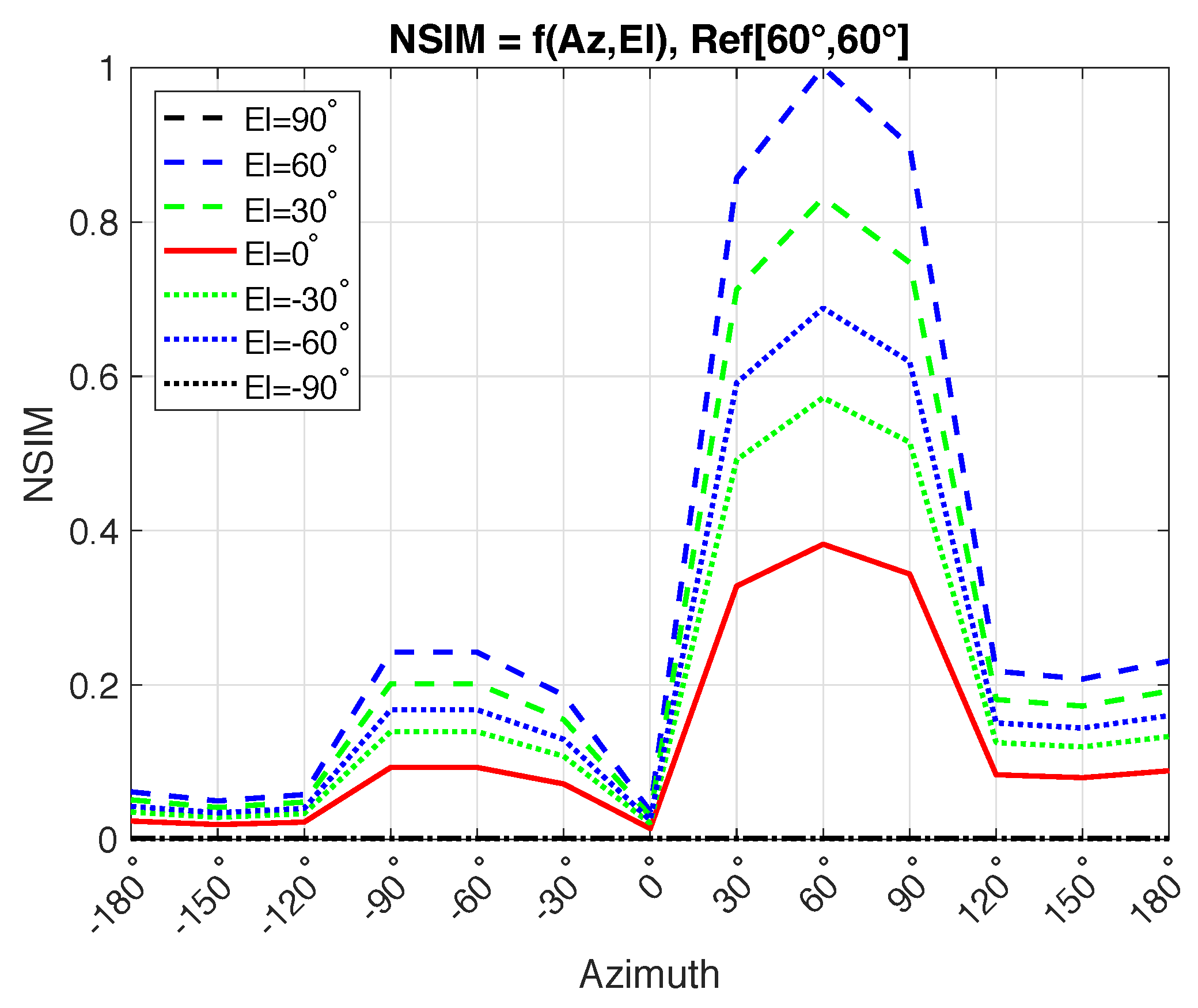
Figure 14 presents the predictions for the same example reference source. Localization accuracy, , is plotted as a function of azimuth (i.e., from −180 to 180 at 30 angle steps) and 7 elevation angles (i.e., from −90 to 90 in 30 angle steps).
The procedure was repeated for 22 fixed reference audio source locations. Figure 15 shows localization accuracy predictions on a sphere where the reference audio source was located at 30 azimuth and 30 elevation and Figure 16 presents the predictions as a function of azimuth and elevation angles.
Validation testing conforms that as the test audio source moves away from the reference audio source, localization accuracy can be seen to decrease monotonically. This was validated using test signals rendered on a sphere. A point of inflection is reached at around ±90 angle in relation to the audio source localization which corresponds to human localization at ±90.
5.2. Multi-Point Sound Sources
We evaluated whether the proposed AMBIQUAL algorithm can accurately predict localization accuracy of multiple point sound sources which were used earlier in MUSHRA subjective tests (see Section 4.6). Aggregated AMBIQUAL localization accuracy scores by encoding schemes with 95% confidence intervals are shown in Figure 12d.
AMBIQUAL localization accuracy scores were compared with subjective MUSHRA scores. Scatter of AMBIQUAL vs. MUSHRA results is presented in Figure 12f (per encoding scheme) and Figure 12h (per sample type). Like before, results show good correlation between objective AMBIQUAL and subjective MUSHRA quality scores (Pearson corr = 0.864, Spearman corr = 0.883).
6. Discussion and Ongoing Work
AMBIQUAL has been shown to be capable of predicting spatial audio QoE in terms of both localization accuracy and listening quality. Both single point and multiple point sound source experiments show good correlation between objective model predictions and subjective MUSHRA scores (see Table 6). Future work will be focused on more complex sound scenes.
The trends exhibited in the aggregated subjective results (as shown in Figure 11a and Figure 12a,b) are replicated by the aggregated objective results (as shown in Figure 11b and Figure 12c,d). This is true for both single and multiple point audio sources for all conditions tested.
It can be seen that the model can predict the difference in quality independently of the test sample content. This is apparent by inspecting the clustering of data points by condition (i.e., bitrate and compression scheme). It is evident for both single point audio sources as shown in Figure 12e and multiple point audio sources as shown in Figure 12f. This observation is further reinforced by the lack of clustering by sample type presented in the two scatter plots in Figure 12g,h.
In this paper, we have presented the AMBIQUAL algorithm which is still at an early developmental stage. The authors are aware that the experiments presented are limited in scope in terms of source number (one or two) and codec used (Opus 1.2) but work is ongoing to test more realistic scenarios with a wider range of compression schemes which share spatial information across the Ambisonics channels.
In [3], a discussion about how listeners judge listening quality and localization accuracy from a QoE perspective is presented. More specifically, can localization accuracy and listening quality be judged independently, or do listeners penalize listening scores if there are localization accuracy issues? This remains an open question. In current research, spatial audio is characterized using a variety of spatial and non-spatial attributes. The weighting factors shown in Figure 10 have been empirically derived. It would be interesting to explore how the directivity associated with the corresponding spherical harmonics contribute to the perceived localization accuracy results and more general models of localization selectivity. Spatial attributes include scene depth and localization accuracy while non-spatial attributes include brilliance and distortion. As such, investigators need to decide whether or not to include non-spatial attributes in quality assessment [40]. State-of-the-art methods from multidimensional quality assessment [23] are recommended until relevant standards are agreed upon.
AMBIQUAL represents a simpler alternative to existing methods of assessing Ambisonics spatial audio. Such methods carry out assessment on binaural renders of several head positions which is not as appealing as AMBIQUAL, which can assess spatial audio quality directly from the Ambisonics format. These early results and the computational simplicity of the method support the proposed further research which will generalize and optimize the approach for higher-order Ambisonics formats.
Author Contributions
M.N., J.S., A.A., M.C. and A.H. contributed equally to conceptualization. M.N. and A.H. contributed equally to the methodology, software, validation, formal analysis and data curation. All authors contributed to writing, reviewing and editing. A.H. was responsible for funding acquisition, project administration and supervision. All authors have read and agreed to the published version of the manuscript.
Acknowledgments
This publication has emanated from research supported by Google LLC. and in part by a research grant from Science Foundation Ireland (SFI) and is co-funded under the European Regional Development Fund under Grant Number 13/RC/2077 and 12/RC/2289_P2.
Conflicts of Interest
Jan Skoglund, Andrew Allen, Michael Chinen are employed by Google LLC. which part funded this research.
References
- Gerzon, M.A. Ambisonics in multichannel broadcasting and video. J. Audio Eng. Soc. 1985, 33, 859–871. [Google Scholar]
- Brettle, J.; Skoglund, J. Open-Source Spatial Audio Compression for VR Content. In Proceedings of the SMPTE 2016 Annual Technical Conference and Exhibition, Los Angeles, CA, USA, 25–27 October 2016; pp. 1–9. [Google Scholar] [CrossRef]
- Narbutt, M.; Skoglund, J.; Allen, A.; Hines, A. Streaming VR for Immersion: Quality aspects of Compressed Spatial Audio. In Proceedings of the 2017 23rd International Conference on Virtual System Multimedia (VSMM), Dublin, Ireland, 31 October–4 November 2017. [Google Scholar]
- Narbutt, M.; Skoglund, J.; Allen, A.; Chenin, M.; Hines, A. Ambiqual—A full reference objective quality metric for ambisonic spatial audio. In Proceedings of the Tenth International Conference on Quality of Multimedia Experience (QoMEX), Cagliari, Italy, 29 May–1 June 2018; IEEE: Piscataway, NJ, USA, 2018; pp. 1–6. [Google Scholar]
- Siddig, A.; Ragano, A.; Jahromi, H.Z.; Hines, A. Fusion confusion: Exploring ambisonic spatial localisation for audio-visual immersion using the McGurk effect. In Proceedings of the 11th ACM Workshop on Immersive Mixed and Virtual Environment Systems, Amherst, MA, USA, 18 June 2019; pp. 28–33. [Google Scholar]
- Zotter, F.; Frank, M. Ambisonics, A Practical 3D Audio Theory for Recording, Studio Production, Sound Reinforcement, and Virtual Reality; Springer: Berlin/Heidelberg, Germany, 2019. [Google Scholar]
- Bertet, S.; Daniel, J.; Parizet, E. Investigation on Localisation Accuracy for First and Higher Order Ambisonics Reproduced Sound Sources. Acta Acust. United Acust. 2013, 99, 642–657. [Google Scholar] [CrossRef] [Green Version]
- Rudzki, T.; Gomez-Lanzaco, I.; Stubbs, J.; Skoglund, J.; Murphy, D.T.; Kearney, G. Auditory Localization in Low-Bitrate Compressed Ambisonic Scenes. Appl. Sci. 2019, 9, 2618. [Google Scholar] [CrossRef] [Green Version]
- Valin, J.M.; Vos, K.; Terriberry, T. Definition of the Opus Audio Codec; IETF: Fremont, CA, USA, 2012. [Google Scholar]
- Valin, J.M.; Bran, C. WebRTC Audio Codec and Processing Requirements; IETF: Fremont, CA, USA, 2016. [Google Scholar]
- Skoglund, J.; Graczyk, M. IETF Internet-Draft: Ambisonics in an Ogg Opus Container; IETF: Fremont, CA, USA, 2017. [Google Scholar]
- Yan, Z.; Wang, J.; Li, Z. A Multi-criteria Subjective Evaluation Method for Binaural Audio Rendering Techniques in Virtual Reality Applications. In Proceedings of the 2019 IEEE International Conference on Multimedia & Expo Workshops (ICMEW), Shanghai, China, 8–12 July 2019; IEEE: Piscataway, NJ, USA, 2019; pp. 402–407. [Google Scholar]
- Fleßner, J.H.; Biberger, T.; Ewert, S.D. Subjective and Objective Assessment of Monaural and Binaural Aspects of Audio Quality. IEEE/ACM Trans. Audio Speech Lang. Process. 2019, 27, 1112–1125. [Google Scholar] [CrossRef]
- Rudzki, T.; Gomez-Lanzaco, I.; Hening, P.; Skoglund, J.; McKenzie, T.; Stubbs, J.; Murphy, D.; Kearney, G. Perceptual Evaluation of Bitrate Compressed Ambisonic Scenes in Loudspeaker Based Reproduction. In Proceedings of the Audio Engineering Society Conference: 2019 AES International Conference on Immersive and Interactive Audio, York, UK, 27–29 March 2019; Audio Engineering Society: New York, NY, USA, 2019. [Google Scholar]
- ITU. ITU-R Rec. P.863: Perceptual Objective Listening Quality Assessment; Int. Telecomm. Union: Geneva, Switzerland, 2014. [Google Scholar]
- Hines, A.; Skoglund, J.; Kokaram, A.C.; Harte, N. ViSQOL: An objective speech quality model. EURASIP J. Audio Speech Music Process. 2015, 2015, 1. [Google Scholar] [CrossRef] [Green Version]
- Thiede, T.; Treurniet, W.C.; Bitto, R.; Schmidmer, C.; Sporer, T.; Beerends, J.G.; Colomes, C. PEAQ-The ITU standard for objective measurement of perceived audio quality. J. Audio Eng. Soc. 2000, 48, 3–29. [Google Scholar]
- Hines, A.; Gillen, E.; Kelly, D.; Skoglund, J.; Kokaram, A.; Harte, N. ViSQOLAudio: An objective audio quality metric for low bitrate codecs. J. Acoust. Soc. Am. 2015, 137, EL449–EL455. [Google Scholar] [CrossRef] [PubMed] [Green Version]
- Kämpf, S.; Liebetrau, J.; Schneider, S.; Sporer, T. Standardization of PEAQ-MC: Extension of ITU-R BS.1387-1 to Multichannel Audio. In Proceedings of the Audio Engineering Society Conference: 40th International Conference: Spatial Audio: Sense the Sound of Space, Tokyo, Japan, 8–10 October 2010; Audio Engineering Society: New York, NY, USA, 2010. [Google Scholar]
- ITU. ITU-R Rec. P.800: Methods for Subjective Determination of Transmission Quality; Int. Telecomm. Union: Geneva, Switzerland, 1996. [Google Scholar]
- ITU. ITU-R Rec. BS.1534-3: Subjective Assessment of Sound Quality; Int. Telecomm. Union: Geneva, Switzerland, 2015. [Google Scholar]
- ITU. ITU-T Rec. BS.1116-3: Methods for the Subjective Assessment of Small Impairments in Audio Systems; Int. Telecomm. Union: Geneva, Switzerland, 2015. [Google Scholar]
- ITU. ITU-T Rec. P.1310: Spatial Audio Meetings Quality; Int. Telecomm. Union: Geneva, Switzerland, 2017. [Google Scholar]
- A MUSHRA Compliant Web Audio API Based Experiment Software. Available online: https://github.com/audiolabs/webMUSHRA (accessed on 4 April 2020).
- Kronlachner, M. AmbiX v0.2.10–Ambisonic Plug-In Suite. 2015. Available online: http://www.matthiaskronlachner.com/?p=2015 (accessed on 4 April 2020).
- SADIE II Database, Binaural and Anthropomorphic Measurements for Virtual Loudspeaker Rendering. 2018. Available online: https://www.york.ac.uk/sadie-project/database.html (accessed on 4 April 2020).
- EBU Tech. 3253-E, Sound quality assessment material. In SQUAM CD (Handbook); EBU Technical Centre Brussels: Grand-Saconnex, Switzerland, 1988. [Google Scholar]
- Hines, A.; Gillen, E.; Kelly, D.; Skoglund, J.; Kokaram, A.; Harte, N. Perceived Audio Quality for Streaming Stereo Music. In Proceedings of the 22nd ACM International Conference on Multimedia, Orlando, FL, USA, 3–7 November 2014; ACM: New York, NY, USA, 2014; pp. 1173–1176. [Google Scholar]
- Gorzel, M.; Allen, A.; Kelly, I.; Kammerl, J.; Gungormusler, A.; Yeh, H.; Boland, F. Efficient encoding and decoding of binaural sound with resonance audio. In Proceedings of the AES International Conference on Immersive and Interactive Audio, York, UK, 27–29 March 2019; Audio Engineering Society: New York, NY, USA, 2019. [Google Scholar]
- Harte, N.; Gillen, E.; Hines, A. TCD-VoIP, a research database of degraded speech for assessing quality in VoIP applications. In Proceedings of the 2015 7th International Workshop on Quality of Multimedia Experience, QoMEX 2015, Pylos-Nestoras, Greece, 26–29 May 2015. [Google Scholar]
- Hines, A.; Harte, N. Speech Intelligibility prediction using a Neurogram Similarity Index Measure. Speech Commun. 2012, 54, 306–320. [Google Scholar] [CrossRef]
- Wang, Z.; Bovik, A.C.; Sheikh, H.R.; Simoncelli, E.P. Image Quality Assessment: From Error Visibility to Structural Similarity. IEEE Trans. Image Process. 2004, 13, 600–612. [Google Scholar] [CrossRef] [PubMed] [Green Version]
- Sloan, C.; Harte, N.; Kelly, D.; Kokaram, A.C.; Hines, A. Objective Assessment of Perceptual Audio Quality Using ViSQOLAudio. IEEE Trans. Broadcast. 2017, 63, 1–13. [Google Scholar] [CrossRef] [Green Version]
- Rayleigh, L. XII. On our perception of sound direction. Lond. Edinb. Dublin Philos. Mag. J. Sci. 1907, 13, 214–232. [Google Scholar] [CrossRef] [Green Version]
- Park, M.; Nelson, P.A.; Kang, K. A model of sound localisation applied to the evaluation of systems for stereophony. Acta Acust. United Acust. 2008, 94, 825–839. [Google Scholar] [CrossRef]
- Yost, W.A. Fundamentals of Hearing: An Introduction; Koninklijke Brill NV: Leiden, The Netherlands, 2013. [Google Scholar]
- Moreau, S.; Daniel, J.; Bertet, S. 3D Sound Field Recording with Higher Order Ambisonics–Objective Measurements and Validation of a 4th order Spherical Microphone. In Proceedings of the Audio Engineering Society 120th Convention, Paris, France, 20–23 May 2006. [Google Scholar]
- Merimaa, J. Analysis, Synthesis, and Perception of Spatial Sound: Binaural Localization Modeling and Multichannel Loudspeaker Reproduction; Helsinki University of Technology: Espoo, Finland, 2006. [Google Scholar]
- Tervo, S. Direction estimation based on sound intensity vectors. In Proceedings of the 17th European Signal Processing Conference, Glasgow, UK, 24–28 August 2009; pp. 700–704. [Google Scholar]
- Zacharov, N.; Pike, C.; Melchior, F.; Worch, T. Next generation audio system assessment using the multiple stimulus ideal profile method. In Proceedings of the Quality of Multimedia Experience (QoMEX), 2016 Eighth International Conference, Lisbon, Portugal, 6–8 June 2016. [Google Scholar]
Figure 1.
Ambisonics spherical harmonics for orders up to three. FOA includes the top two lines of basis functions (4 channels) and 3OA includes all four lines (16 channels). The ACN channels 2, 6 and 12 contain only vertical components.
Figure 1.
Ambisonics spherical harmonics for orders up to three. FOA includes the top two lines of basis functions (4 channels) and 3OA includes all four lines (16 channels). The ACN channels 2, 6 and 12 contain only vertical components.

Figure 2.
WebMUSHRA Graphical User Interface.

Figure 3.
Single point audio source localization: (a) fixed position (azimuth 60, elevation 60), (b) audio source moving horizontally above the listener’s head, (c) audio source moving up in elevation on the left hand side, then down on the right hand side. Reproduced from [3].
Figure 3.
Single point audio source localization: (a) fixed position (azimuth 60, elevation 60), (b) audio source moving horizontally above the listener’s head, (c) audio source moving up in elevation on the left hand side, then down on the right hand side. Reproduced from [3].

Figure 4.
Localizations of multiple point audio sources: (a,b,d) one source with fixed localization and one with dynamic azimuth localization moving horizontally (i.e., rotating above or below the listener’s head), (c,e,f) one source with fixed localization and one with the audio source moving up in elevation on the left hand side, then down on the right hand side.

Figure 5.
NSIM scores derived from the Similarity Map between Reference and Test Gammmatonegrams. Further examples and descriptions can be found in [33].
Figure 5.
NSIM scores derived from the Similarity Map between Reference and Test Gammmatonegrams. Further examples and descriptions can be found in [33].

Figure 6.
Interaural Time Difference (ITD) and Interaural Level Difference (ILD) between left and right ears.
Figure 6.
Interaural Time Difference (ITD) and Interaural Level Difference (ILD) between left and right ears.

Figure 7.
Phaseograms, similarity map, and similarity scores for 100 Hz pure sine wave signals. The Reference signal is localized at Azimuth = 60, Elevation = 60, the Test signal at Azimuth = 50, Elevation = 60 and resulting localization accuracy score is 0.944.
Figure 7.
Phaseograms, similarity map, and similarity scores for 100 Hz pure sine wave signals. The Reference signal is localized at Azimuth = 60, Elevation = 60, the Test signal at Azimuth = 50, Elevation = 60 and resulting localization accuracy score is 0.944.

Figure 8.
Phaseograms, similarity map, and similarity scores for 100 Hz pure sine wave signals. The Reference signal is localized at Azimuth = 60, Elevation = 60, the Test signal at Azimuth = 10, Elevation = 60 and resulting localization accuracy score is 0.918.
Figure 8.
Phaseograms, similarity map, and similarity scores for 100 Hz pure sine wave signals. The Reference signal is localized at Azimuth = 60, Elevation = 60, the Test signal at Azimuth = 10, Elevation = 60 and resulting localization accuracy score is 0.918.

Figure 9.
Channel occupancy of B-format Ambisonics audio as a function of azimuth (AZ) and elevation (EL) of sound sources. Empty channels are represented here with the ‘x’ sign.
Figure 9.
Channel occupancy of B-format Ambisonics audio as a function of azimuth (AZ) and elevation (EL) of sound sources. Empty channels are represented here with the ‘x’ sign.

Figure 10.
Values of weighting factors that maximize correlation between AMBIQUAL results and subjective MUSHRA scores.
Figure 10.
Values of weighting factors that maximize correlation between AMBIQUAL results and subjective MUSHRA scores.

Figure 11.
Listening quality-subjective vs. AMBIQUAL results for single point audio sources: (a) aggregated subjective results and (b) AMBIQUAL quality predictions by encoding scheme (mean values with 95% confidence intervals shown) and scatter of subjective scores vs. AMBIQUAL results by encoding scheme (c) and by sample type (d).

Figure 12.
Localization accuracy-subjective vs. AMBIQUAL results: (a,b) aggregated subjective localization accuracy scores by encoding scheme (one point audio sources and multi-point audio sources respectively) showing mean values with 95% confidence intervals shown. Plots (c,d) show aggregated AMBIQUAL results by encoding scheme (one and multi-point sources respectively). Plots (e,f) scatter of subjective vs. AMBIQUAL results by encoding (one and multi-point sources respectively), (g,h) scatter of subjective vs. AMBIQUAL results by sample type (one and multi-point sources respectively).

Figure 13.
Localization accuracy scores distributed on a sphere. The reference audio source was localized at azimuth = 60, elevation = 60 (the red circle represents the reference audio source). Reproduced from [4].
Figure 13.
Localization accuracy scores distributed on a sphere. The reference audio source was localized at azimuth = 60, elevation = 60 (the red circle represents the reference audio source). Reproduced from [4].

Figure 14.
Localization accuracy as a function of azimuth and elevation with fixed reference audio source, localized at an offset point of azimuth = 60, elevation = 60. The asymmetry in the results is caused by the source being closer to one ear than the other. Reproduced from [4].
Figure 14.
Localization accuracy as a function of azimuth and elevation with fixed reference audio source, localized at an offset point of azimuth = 60, elevation = 60. The asymmetry in the results is caused by the source being closer to one ear than the other. Reproduced from [4].

Figure 15.
Localization accuracy scores distributed on a sphere. In this case, the reference audio source was localized at azimuth = 30, elevation = 30 (the red circle represents the reference audio source).
Figure 15.
Localization accuracy scores distributed on a sphere. In this case, the reference audio source was localized at azimuth = 30, elevation = 30 (the red circle represents the reference audio source).

Figure 16.
Localization accuracy as a function of azimuth and elevation. A fixed reference audio source is located at an offset point of azimuth = 30, elevation = 30. The asymmetry in results is caused by the source being closer to one ear than the other.
Figure 16.
Localization accuracy as a function of azimuth and elevation. A fixed reference audio source is located at an offset point of azimuth = 30, elevation = 30. The asymmetry in results is caused by the source being closer to one ear than the other.


Table 1.
Samples used during single point audio listening tests (reproduced from [3]).
Table 1.
Samples used during single point audio listening tests (reproduced from [3]).
| Label | Music Type | Source |
|---|---|---|
| vega | Vocals (Suzanne Vega) | CD |
| castanets | Castanets | EBU |
| glock | Glockenspiel | EBU |
| vegaRev | Vocals (Suzanne Vega) w. Reverb effect | processed CD |
| castanetsRev | Castanets w. Reverb Effect | processed EBU |
| pinkRev | Bursty Pink Noise w. Reverb Effect | synthetic |
Table 2.
Azimuth and elevation angles in degrees used for 26-point Lebedev Quadrature layout.
| Elevation | ±35 | ±35 | ±45 | ±45 | ±90 | 0 | 0 | 0 | 0 | 0 |
| Azimuth | ±135 | ±45 | 0 | 180 | 0 | 0 | ±135 | 180 | ±45 | ±90 |
Table 3.
Encoding/compression schemes used with single point audio sources.
| Ambisonics | Bit Rate | Bit Rate Per | |
|---|---|---|---|
| Type | Order | (kbps) | Channel (kbps) |
| Reference | 3 | 12,288 | 768 |
| 3OA 512 | 3 | 512 | 32 |
| 3OA 256 | 3 | 256 | 16 |
| FOA 128 | 1 | 128 | 32 |
| FOA 32 (anchor) | 1 | 32 | 8 |
Table 4.
Multiple point audio samples used during listening tests.
| Label | Music Type | Source |
|---|---|---|
| castanetsRev | Castanets w. Reverb Effect | processed EBU |
| pinkRev | Bursty Pink Noise w. Reverb Effect | synthetic |
| tub | Tubular bells | EBU |
| xyl | Xylophone | EBU |
| fem | Female voice | EBU |
| babble | Babble noise | TCDVOIP |
| tr | Triangle | EBU |
| piano | Piano | EBU |
Table 5.
Encoding/compression schemes used with multiple point audio sources.
| Ambisonics | Bit Rate | Bit Rate Per | |
|---|---|---|---|
| Type | Order | (kbps) | Channel (kbps) |
| Reference | 3 | 12,288 | 768 |
| 3OA 512 | 3 | 512 | 32 |
| 3OA 384 | 3 | 384 | 24 |
| 3OA 256 | 3 | 256 | 16 |
| FOA 128 | 1 | 128 | 32 |
| FOA 96 | 1 | 96 | 24 |
| FOA 64 | 1 | 64 | 16 |
| FOA 32 (anchor) | 1 | 32 | 8 |
Table 6.
Correlation between subjective MUSHRA and objective AMBIQUAL results from experiments 1 and 2.
Table 6.
Correlation between subjective MUSHRA and objective AMBIQUAL results from experiments 1 and 2.
| Listening Quality | Localization Accuracy | |||||
|---|---|---|---|---|---|---|
| Pearson | Spearman | RMSE | Pearson | Spearman | RMSE | |
| 1 | 0.899 | 0.816 | 55.14 | 0.922 | 0.919 | 59.27 |
| 2 | - | - | - | 0.864 | 0.883 | 63.13 |
© 2020 by the authors. Licensee MDPI, Basel, Switzerland. This article is an open access article distributed under the terms and conditions of the Creative Commons Attribution (CC BY) license (http://creativecommons.org/licenses/by/4.0/).
Share and Cite
MDPI and ACS Style
Narbutt, M.; Skoglund, J.; Allen, A.; Chinen, M.; Barry, D.; Hines, A. AMBIQUAL: Towards a Quality Metric for Headphone Rendered Compressed Ambisonic Spatial Audio. Appl. Sci. 2020, 10, 3188. https://doi.org/10.3390/app10093188
AMA Style
Narbutt M, Skoglund J, Allen A, Chinen M, Barry D, Hines A. AMBIQUAL: Towards a Quality Metric for Headphone Rendered Compressed Ambisonic Spatial Audio. Applied Sciences. 2020; 10(9):3188. https://doi.org/10.3390/app10093188
Chicago/Turabian StyleNarbutt, Miroslaw, Jan Skoglund, Andrew Allen, Michael Chinen, Dan Barry, and Andrew Hines. 2020. "AMBIQUAL: Towards a Quality Metric for Headphone Rendered Compressed Ambisonic Spatial Audio" Applied Sciences 10, no. 9: 3188. https://doi.org/10.3390/app10093188
Note that from the first issue of 2016, this journal uses article numbers instead of page numbers. See further details here.