Towards Piston Fine Tuning of Segmented Mirrors through Reinforcement Learning


1
Universidad de La Laguna, C/ Padre Herrera s/n., 38200 La Laguna, Spain
2
Wooptix, S.L. Avda. Trinidad 61, 38204 La Laguna, Spain
3
ITB, Campus Ciencias de La Salud s/n, E-38071 La Laguna, Spain
*
Author to whom correspondence should be addressed.
Appl. Sci. 2020, 10(9), 3207; https://doi.org/10.3390/app10093207
Submission received: 7 April 2020
/
Revised: 30 April 2020
/
Accepted: 30 April 2020
/
Published: 4 May 2020
(This article belongs to the Section Optics and Lasers)
Abstract
:Featured Application
Piston alignment of segmented optical mirror telescopes through an algorithm that learns by itself how to maximize a physical quantity of the system.
Abstract
Unlike supervised machine learning methods, reinforcement learning allows an entity to learn how to deploy a task from experience rather than labeled data. This approach has been used in this paper to correct piston misalignment between segments in a segmented mirror telescope. It was proven in simulations that the algorithm converges to a point where it learns how to move the piston actuators in order to maximize the Strehl ratio of the wavefront at the intersection.
1. Introduction
It is desirable to shorten the observation time needed by a terrestrial telescope to obtain a certain signal-to-noise ratio. In a diffraction limited scenario, it is inversely proportional to the fourth power of the diameter of the aperture. Hence, there is plenty of motivation for constructing larger telescopes. Successful construction of telescopes of 8 m and larger has been possible to a large extent with the introduction of segmented mirrors. To build telescopes with monolithic mirrors of the same size would have been impractical for financial and physical reasons. However, that segmentation in the reflective surface also introduced novel complications. A large increase in the number of parts and complexity of the system is one of these drawbacks. Piston errors introduce phase shifts between segments. Adjusting the degrees of freedom to mitigate these errors is problematic since they do not produce a slope in the wavefront.
Several methods have been developed in recent decades to tackle the problem of piston misalignment. The ones that are most currently used are based on Shack–Hartman wavefront sensors [1,2]. These methods rely on intensity images measured at the pupil plane. They have been proven to be reliable and precise. However, they require each segment edge to be aligned on a lenslet grid and this process might be very time-consuming. There is other family of methods that uses curvature sensors. These methods measure intensities at intermediate planes between pupil and focus. They are used to crosscheck the measurements obtained by the main methods. They are robust and require little extra hardware, but their capture range is not very large and they are deeply constrained by atmospheric conditions [3,4].
Other methods that have been proposed recently employ convolutional neural networks. This paradigm of machine learning has seen nowadays a great host of applications in many different areas. Some of the methods proposed so far are only suitable for extended objects [5] or have not been proven to be robust under atmospheric turbulence [6].
As far as we are concerned, all machine learning applications to piston sensing so far stand on the supervised paradigm [7,8,9]. In this setting, input data and target have to be supplied. This requires the algorithm to be trained on simulated image data as well as the exact piston values. Eventually, the correspondence between the two sets is found after giving enough training data and enough model capacity. Nevertheless, the probability distributions of both, the synthetic and the real world data, must be in accordance with each other in order to generalize well in a real environment.
The technique presented here takes a reinforcement learning approach. It means that the learning process is driven by experience in an environment rather than training on a previously labeled dataset. It is then suitable for scenarios where ground-truth-labeled data are scarce or difficult to obtain. In the optical phasing problem, real telescope diffraction images might be available. However they lack the exact piston values that gave rise to those images. The RL algorithm learns in place with data provided by the telescope mirror in real time. Furthermore, it relies on an external physical quantity rather than labels. The method employs a convolutional neural network that takes as input an intensity image measured at an intermediate plane with four different wavelengths. The network outputs a probability distribution over actions that the piston actuators can take to reach an optimum Strehl ratio at the intersection. The agent then executes an action sampled from that distribution on the environment. Additionally, an image of the PSF of the portion of the wavefront at the given intersection is needed only during training. Once the network has been trained, this method gives fast immediate piston correction that could be used at any time during the observation. In supervised learning approaches, the PSF images are not needed; synthetic diffraction images are used instead.
The method has also been tested under atmospheric turbulence. The diffraction image was filtered with the long exposure optical transfer function. A Fried parameter of was considered in the simulations.
Large scale metrology approaches can be used jointly with this RL fine tuning approach. The former allows characterizing the position and orientation of each mirror segment by means of photogrammetry or laser tracker technology [10,11,12,13].
The paper is organized as follows. First, the physical details of the problem and its mathematical considerations are introduced briefly. Then, there is the optical setup and the procedure to generate the simulations to continue in the next part with an introduction to the policy gradients method and the architecture of the network. Finally, conclusions and final remarks are found at the end of the paper.
2. Background
The electromagnetic field emitted by a distant point source of light such as a star reaches the pupil of the telescope in the form of a plane wave. However, aberrations from either the propagation medium or the telescope itself make the wavefront depart from this ideal view. For simplicity, it is taken into consideration only the region of the wavefront reflected in three adjacent segments on a three ring segmented hexagonal mirror. There is piston misalignment in between the segments that introduces discontinuities in the phase of the wavefront. Figure 1 shows an intensity image recorded at the detector plane produced by the wavefront just described.
The intensity of the field is recorded at a distance , away from the focus with four different wavelengths. This distance is such that the full peak width of the diffraction pattern is twice larger than the image blur due to the atmospheric turbulence, as explained here [14]. The focal length of the telescope is set to be .
Four different wavelengths are considered to give the network the ability to distinguish piston errors that surpass the ambiguity range [15]. The largest is taken as the reference wavelength and three shorter ones to disambiguate , and . All piston values throughout the paper are measured at the wavefront. If a single wavelength would be used instead, diffraction patterns would be periodic with respect to the piston step values and the algorithm would not be able to predict which one gave rise to those images.
The wavefront at the pupil propagates to the observation plane by means of Fresnel equation. The observation plane is located at a distance z from the pupil. The distance z can be related to the focal length f, and the defocus distance d through Newton lens formula .
The intensity distribution at the observation plane is the squared magnitude of the complex field after propagation. Eventually, an image like the one in Figure 2 is produced.
The study takes also into consideration the atmospheric turbulence effects. The simulated intensity image at the defocus plane is filtered with the long exposure transfer function of the atmosphere [16]. A value for Fried parameter of was chosen.
Table 1 displays a summary of the parameters used in the simulation.
3. Results and Methodology
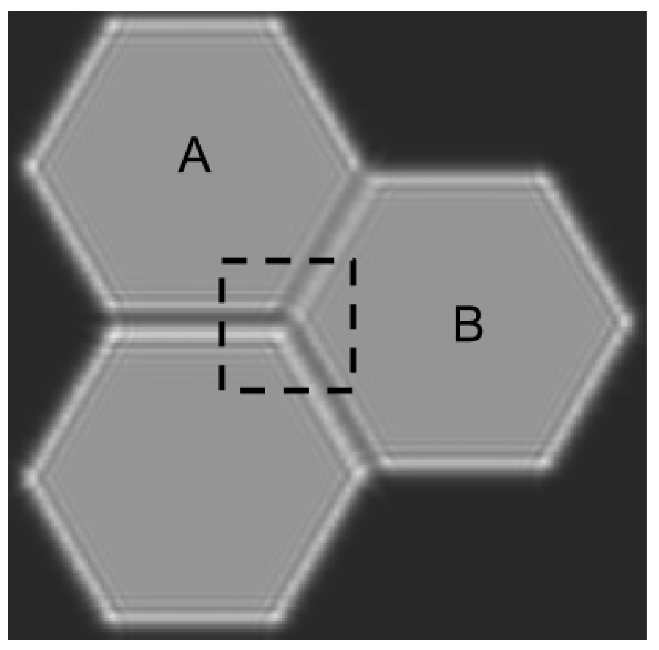
Reinforcement learning is a subfield of machine learning in which an algorithm gets feedback from the environment in the form of reward or punishment. According to this approach, the optimization problem becomes how to design an agent that acts optimally to get the highest long-term expected reward from the environment. Or alternatively, in the specific domain of optical phasing, given a diffraction image of an intersection of three adjacent segments, how to move piston actuators A and B in Figure 2 in order to get the maximum Strehl ratio of the wavefront at the intersection.
In a reinforcement learning setup, it is helpful to model the problem as a Markov Decision Process (MDP) in which the following tuple of elements have to be defined.
The set of states the agent can be at, , are the diffraction images of the intersection of the segments taken at four different wavelengths. It is shown with dashed line in Figure 2. It is a pixels image around the center of the intersection. It is assumed that tip-tilt values have been restored for each segment in a previous stage, hence only piston values remain.
The actions, U, are the set of all possible piston movements that can be commanded to segments A and B. These are pairs of values with units of length. They are limited to a distance equivalent to , being the reference wavelength. Since only piston steps in the range are considered, it is assumed that those action values should be enough to correct the piston misalignment completely. It might be the case that after movements have been applied to both A and B segments pistons, the final piston error among them might lie outside the limit. Using four wavelengths helps to distinguish states outside the ambiguity range.
The element P is the transition probability. It is the probability of ending at a final state conditioned on both, an initial state and a certain action, . They are the stochastic rules that govern the physics of the environment, i.e., the probability distribution over states that can be reached from initial state when a certain action is taken. It corresponds to the dynamics of the system and it is implicitly learned by the algorithm through experience.
The reward signal, R, is obtained when taking action at state . The sum of the maximum intensity values of the PSF images for each wavelength at the intersection is used as the reward. This value is proportional to the Strehl ratio. In order to produce the intersection PSF, a circular mask is first placed at the center of the junction of the three segments. That mask isolates a circular portion of the wavefront. The diameter of the mask is equivalent to at the pupil. The reward is deterministic in the simulations. However, it can be considered stochastic in a general RL setup, as long as the expected long-term reward defines the agent final goal. The algorithm aims to maximize the expected long-term value of these reward outcomes.
And last, the discount factor is used in a sequential task to indicate how valuable it is to achieve the rewards as soon as possible. In the one step MDP case, this hyperparameter is set to zero. This means that the agent only cares about the immediate reward. A one step MDP is shown diagrammatically in Figure 1.
Figure 3 represents the phase of the wavefront centered at the intersection after the circular mask has been applied. It is interesting to notice that the diameter of the wavefront is only sampled by ten pixels in the simulation. On the right hand side of the same figure, the PSF image of that part of the wavefront is showed. In a physical setup, that can be achieved by placing a microlens array centered at each segment junction. The PSF is obtained for each of the four wavelengths. The mask would be only needed during training.
The goal is to find the best possible policy such that the final expected reward is maximized. The policy gives a probability distribution over actions that the piston actuators can take from a given state. It can be represented with a three layer convolutional neural network where is the set of parameters to be tuned. Each convolutional layer has 16 filters with weights and ReLU activation function. The sizes of the filters are , , at each layer respectively. The depth of each filter matches the previous activation depth. A trainable bias parameter for each filter is also considered in the network. A fully connected layer is placed at the end to compute the final scores. The output of the network defines the mean of a bivariate probability normal distribution over actions. This mean is the action that is more likely to achieve the highest long-term reward from the current state, according to the agent experience. An action sampled from that distribution comprises two length components to be commanded to both pistons, A and B. Sampling the action from the normal distribution rather than selecting the mean predicted by the network allows the agent to explore nearby actions that might end up being a better option than the prediction itself. Since the absolute piston positions are unknown, the actions represent the relative piston movement from initial to final state.
The quantity to be optimized is called utility and it can be expressed mathematically by the following manner:
where is the probability of the state and the action under a particular policy. And is the reward. The gradient of the utility of the policy parameters can be approximated with an empirical estimate for m samples [17]:
where m is the number of trials used in the estimation of the gradient.
A Gaussian model is used to describe a stochastic policy over the continuous action space. The mean of the Gaussian is where the agent thinks that lies the action that is more likely to give the highest long-term expected reward from the current state. The variance of the Gaussian quantifies the uncertainty about that prediction. Since the random policy happens to be Gaussian, the form of the gradient of the log-probability turns out to be:
The CNN returns two single scalar values for each diffraction image that it takes as an input. The mean of the bivariate distribution is precisely the output of the convolutional network. The gradient can be computed with respect to its parameters through backpropagation in the usual way. The variance of the distribution is fixed to a small value. However, it can also be parameterized and learned from the experience. The action to be taken by the agent is sampled from that distribution. Selecting actions randomly allows the agent to explore new optimal actions while exploiting the current policy. Now, with the expression of the gradient, the optimum value of the parameters can be found with the gradient ascent. Adam algorithm, a variant of the latter, was used in the simulations [18].
On the other hand, a second convolutional network is used as a function approximator to represent the value function [19], . It takes as input the state i.e., the diffraction image of the intersection, and returns the expected reward from that state under the current policy . The set of parameters that better approximate the value function are learned in a supervised manner from experience.
The value function can be used as a state dependent baseline to reduce the variance of the algorithm [20]. Using the advantage estimator rather than simply the reward in the Equation (2) makes the learning process more stable. Using the baseline function makes the variance decrease without changing the expectation of the gradient.
The capture range defines the interval of possible piston jump values that the agent is trained to detect and act upon. Capture ranges considered here are suitable for fine tuning the piston positions after a previous coarse piston alignment stage has been carried out. The intersection has two piston jumps to segments A and B. Every combination of piston step values generates a distinctive diffraction pattern. The broader the capture range, the more patterns the agent is required to recognize to be able to perform the proper action.
Algorithm 1 shows the complete learning sequence. The initial state is the diffraction image of an intersection with piston jumps from bottom left segment to segments A and B. They can be any random value within the capture range, see Figure 2 for clarity. The policy network takes the diffraction image as input and predicts the mean of a Gaussian over the continuous action space. Then an action is sampled from that distribution in step 4. Next, state and reward are recorded once the action has been performed on the environment in step 5. The advantage is computed in step 6 and it quantifies how good or bad that reward is with respect to the average reward achieved on that state. The expected reward from a state following the policy is given by the value function. In order to be self-consistent, the value of the initial state , must be close on average to the immediate reward plus the value of the final state . The squared distance between the two quantities is a loss function to be minimized. Updating the value function parameters to minimize the loss function is done in step 7. Finally in step 8, policy network parameters are updated in the direction of the log-policy gradient by an amount given by the advantage.
In Figure 4, we can see the training process while running the Algorithm 1. The vertical axis represents the sum of the PSF maximum intensity value for each wavelength after taking the action predicted by the policy. This magnitude has been normalized by the value attained with a perfectly phased intersection. The learning process plateaus at around . This is also the average maximum reward the agent achieves from any initial state. There is an upper bound on this quantity that is imposed by the small fix variance set in the design of the Gaussian policy. Two learning processes are shown in Figure 4. The continuous line represents the agent learning process over a capture range of . On the other hand, the dashed line shows the learning process for piston steps within the range .
| Algorithm 1 Policy gradients with value function baseline |
|
It is interesting to visualize how accurately the network rectifies the piston misalignment during training. It is important to point out that the RL agent does not predict the piston mse error. It rather learns how to minimize it through the optimization of the PSF. In a real scenario, it would not be possible to know the ground truth piston misalignment in the initial state that gave rise to the diffraction image. Yet, it might be known in a simulated environment. Figure 5 shows the evolution of the mean squared error of the predictions over training steps measured in units of . A straight line is plotted at the threshold . Below this value, the intersection is known to have a Strehl ratio greater than [21]. Eventually, the agent gets to align the intersection with an accuracy of on both capture ranges and .
The two graphs shown in Figure 4 and Figure 5 are somehow related. Getting higher reward means in general a better estimation of the piston misalignment. The graphs have been smoothed out with a moving average over the last five steps.
Every step requires a real piston movement in the telescope, so the number of them needed by the agent to learn the task is an important aspect to consider. In that sense, the agent takes fewer steps to learn the task for the capture range . A long exposure image is the result of a large number of atmospheric perturbation realizations. It is necessary to use an exposure time much larger than , depending on wind velocity, in order to capture the time averaging effect of the atmosphere. An exposition time of per image sets a lower bound duration of to reach in capture range . Additionally, a lower bound duration of is set for the agent to reach the same rms value in capture range . The training though can be carried out in parallel at several intersections simultaneously. There are 10 of them to train on in a 36 segment mirror telescope. It makes the previous training times decrease to h and h respectively.
4. Conclusions and Future Work
In this paper, we have shown a novel approach to train convolutional neural networks for cophasing segmented mirrors. Unlike other supervised learning approaches, it does not need the data to be labeled. The maximum of the PSF image of the intersection is used instead. The method is able to correct piston step values in the range . The narrower the capture range, the faster the agent learns. This is why the method is more appropriate for piston fine tuning.
This technique requires us to apply a circular mask centered at the junction of every three segments to obtain the PSF of that part of the wavefront. However, this optical setup aligned with the intersections is only needed during training. This means that once trained, the agent is able to correct piston misalignments in one single forward pass of the network by using the diffraction image alone.
The accuracy attained in the predictions of the optical path difference between segments was for a reference wavelength . This measurement at the wavefront suffices for the adaptive optics to be applied [22].
Quantitative analysis on how seeing variations can influence the training of the RL agent will be treated in future work.
Author Contributions
Conceptualization, D.G.-R.; methodology, D.G.-R.; software, D.G.-R.; validation, J.T.-S. and J.M.R.-R.; formal analysis, J.T.-S. and J.M.R.-R.; investigation, D.G.-R.; resources, J.T.-S. and J.M.R.-R.; data curation, J.T.-S. and J.M.R.-R.; writing—original draft preparation, D.G.-R.; writing—review and editing, J.T.-S. and J.M.R.-R.; visualization, D.G.-R.; supervision, J.T.-S. and J.M.R.-R.; project administration, J.M.R-R. All authors have read and agreed to the published version of the manuscript.
Funding
This research received no external funding.
Acknowledgments
This work was supported by Wooptix, a spinoff company of the Universidad de La Laguna.
Conflicts of Interest
The authors declare no conflict of interest.
Abbreviations
The following abbreviations are used in this manuscript:
| PSF | Point Spread Function |
| MDP | Markov Decision Process |
| CNN | Convolutional Neural Network |
| RL | Reinforcement Learning |
References
- Chanan, G.; Ohara, C.; Troy, M. Phasing the mirror segments of the Keck telescopes II: the narrow-band phasing algorithm. Appl. Opt. 2000, 39, 4706–4714. [Google Scholar] [CrossRef] [PubMed]
- Chanan, G.; Troy, M.; Dekens, F.; Michaels, S.; Nelson, J.; Mast, T.; Kirkman, D. Phasing the mirror segments of the Keck telescopes: the broadband phasing algorithm. Appl. Opt. 1998, 37, 140–155. [Google Scholar] [CrossRef] [PubMed] [Green Version]
- Rodriguez-Ramos, J.M.; Fuensalida, J.J. Piston detection of a segmented mirror telescope using a curvature sensor: Preliminary results with numerical simulations. In Optical Telescopes of Today and Tomorrow; International Society for Optics and Photonics: Bellingham, WA, USA, 1997; Volume 2871, pp. 613–617. [Google Scholar]
- Orlov, V.G.; Cuevas, S.; Garfias, F.; Voitsekhovich, V.V.; Sanchez, L.J. Co-phasing of segmented mirror telescopes with curvature sensing. In Telescope Structures, Enclosures, Controls, Assembly/Integration/Validation, and Commissioning; International Society for Optics and Photonics: Bellingham, WA, USA, 2000; Volume 4004, pp. 540–552. [Google Scholar]
- Li, D.; Xu, S.; Wang, D.; Yan, D. Large-scale piston error detection technology for segmented optical mirrors via convolutional neural networks. Opt. Lett. 2019, 44, 1170–1173. [Google Scholar] [CrossRef] [PubMed]
- Ma, X.; Xie, Z.; Ma, H.; Xu, Y.; Ren, G.; Liu, Y. Piston sensing of sparse aperture systems with a single broadband image via deep learning. Opt. Express 2019, 27, 16058–16070. [Google Scholar] [CrossRef] [PubMed]
- Guerra-Ramos, D.; Díaz-García, L.; Trujillo-Sevilla, J.; Rodríguez-Ramos, J.M. Piston alignment of segmented optical mirrors via convolutional neural networks. Opt. Lett. 2018, 43, 4264–4267. [Google Scholar] [CrossRef] [PubMed]
- Ma, X.; Xie, Z.; Ma, H.; Xu, Y.; He, D.; Ren, G. Piston sensing for sparse aperture systems with broadband extended objects via a single convolutional neural network. Opt. Lasers Eng. 2020, 128, 106005. [Google Scholar] [CrossRef]
- Hui, M.; Li, W.; Liu, M.; Dong, L.; Kong, L.; Zhao, Y. Object-independent piston diagnosing approach for segmented optical mirrors via deep convolutional neural network. Appl. Opt. 2020, 59, 771–778. [Google Scholar] [CrossRef] [PubMed]
- Mutilba, U.; Kortaberria, G.; Egaña, F.; Yagüe-Fabra, J.A. Relative pointing error verification of the Telescope Mount Assembly subsystem for the Large Synoptic Survey Telescope. In Proceedings of the 2018 5th IEEE International Workshop on Metrology for AeroSpace (MetroAeroSpace), Rome, Italy, 20–22 June 2018; pp. 155–160. [Google Scholar]
- Rakich, A. Using a laser tracker for active alignment on the Large Binocular Telescope. In Proceedings of the Ground-Based and Airborne Telescopes IV, Amsterdam, The Netherlands, 1–6 July 2012; International Society for Optics and Photonics: Bellingham, WA, USA, 2012; Volume 8444, p. 844454. [Google Scholar]
- Rakich, A.; Dettmann, L.; Leveque, S.; Guisard, S. A 3D metrology system for the GMT. In Proceedings of the Ground-based and Airborne Telescopes VI, Edinburgh, UK, 26 June–1 July 2016; International Society for Optics and Photonics: Bellingham, WA, USA, 2016; Volume 9906, p. 990614. [Google Scholar]
- Gressler, W.J.; Sandwith, S. Active Alignment System for the LSST. In Proceedings of the Columbia Music Scholarship Conference (CMSC), Orlando, FL, USA, 3–4 February 2006. [Google Scholar]
- Schumacher, A.; Devaney, N. Phasing segmented mirrors using defocused images at visible wavelengths. Mon. Not. R. Astron. Soc. 2006, 366, 537–546. [Google Scholar] [CrossRef] [Green Version]
- Lofdahl, M.G.; Eriksson, H. Algorithm for resolving 2pi ambiguities in interferometric measurements by use of multiple wavelengths. Opt. Eng. 2001, 40, 984–991. [Google Scholar]
- Fried, D.L. Optical resolution through a randomly inhomogeneous medium for very long and very short exposures. JOSA 1966, 56, 1372–1379. [Google Scholar] [CrossRef]
- Williams, R.J. Simple statistical gradient-following algorithms for connectionist reinforcement learning. Mach. Learn. 1992, 8, 229–256. [Google Scholar] [CrossRef] [Green Version]
- Kingma, D.P.; Ba, J. Adam: A Method for Stochastic Optimization. arXiv 2014, arXiv:1412.6980. [Google Scholar]
- Sutton, R.S.; Barto, A.G. Introduction to Reinforcement Learning; MIT press: Cambridge, UK, 1998; Volume 135. [Google Scholar]
- Greensmith, E.; Bartlett, P.L.; Baxter, J. Variance reduction techniques for gradient estimates in reinforcement learning. J. Mach. Learn. Res. 2004, 5, 1471–1530. [Google Scholar]
- Yaitskova, N.; Dohlen, K.; Dierickx, P. Analytical study of diffraction effects in extremely large segmented telescopes. JOSA A 2003, 20, 1563–1575. [Google Scholar] [CrossRef] [PubMed]
- Yaitskova, N. Adaptive optics correction of segment aberration. JOSA A 2009, 26, 59–71. [Google Scholar] [CrossRef] [PubMed]
Figure 1.
Diagram of one step Markov Decision Process.

Figure 2.
Diffraction image of three segments with piston errors between them. Distinctive intensity ripples at the borders between segments are caused by wavefront discontinuities. These discontinuities are, in turn, due to piston errors. Movement orders are commanded to segments A and B to minimize the effects of the errors between the three.

Figure 3.
(a) Wavefront at the intersection once a circular mask has been applied. It contains a portion of the wavefront from each of the three segments. (b) PSF of the previous circular wavefront at the intersection. It is recorded at the focus plane behind the microlens.
Figure 3.
(a) Wavefront at the intersection once a circular mask has been applied. It contains a portion of the wavefront from each of the three segments. (b) PSF of the previous circular wavefront at the intersection. It is recorded at the focus plane behind the microlens.

Figure 4.
Normalized maximum of the PSF reached by the algorithm during training. Capture range of in continuous line and in dashed line.
Figure 4.
Normalized maximum of the PSF reached by the algorithm during training. Capture range of in continuous line and in dashed line.

Figure 5.
Accuracy of actions at predicting ground truth piston discontinuities. Capture range of in continuous line and in dashed line. The RL agent does not predict the mse value itself, rather it learns how to minimize it through the optimization of the PSF. A horizontal line at has been drawn. A system with an rms below that threshold is known to have a Strehl ratio of 0.8 for the given wavelength.


Table 1.
Simulation parameters.
| Parameter | Value |
|---|---|
| Focal length of telescope | |
| Defocus distance | |
| Physical size of segment | |
| Pupil scale at the detector | |
| Fried parameter | |
| Largest wavelength |
© 2020 by the authors. Licensee MDPI, Basel, Switzerland. This article is an open access article distributed under the terms and conditions of the Creative Commons Attribution (CC BY) license (http://creativecommons.org/licenses/by/4.0/).
Share and Cite
MDPI and ACS Style
Guerra-Ramos, D.; Trujillo-Sevilla, J.; Rodríguez-Ramos, J.M. Towards Piston Fine Tuning of Segmented Mirrors through Reinforcement Learning. Appl. Sci. 2020, 10, 3207. https://doi.org/10.3390/app10093207
AMA Style
Guerra-Ramos D, Trujillo-Sevilla J, Rodríguez-Ramos JM. Towards Piston Fine Tuning of Segmented Mirrors through Reinforcement Learning. Applied Sciences. 2020; 10(9):3207. https://doi.org/10.3390/app10093207
Chicago/Turabian StyleGuerra-Ramos, Dailos, Juan Trujillo-Sevilla, and Jose Manuel Rodríguez-Ramos. 2020. "Towards Piston Fine Tuning of Segmented Mirrors through Reinforcement Learning" Applied Sciences 10, no. 9: 3207. https://doi.org/10.3390/app10093207
Note that from the first issue of 2016, this journal uses article numbers instead of page numbers. See further details here.