Predictive Sales and Operations Planning Based on a Statistical Treatment of Demand to Increase Efficiency: A Supply Chain Simulation Case Study

Abstract

Forecasting is the basis for planning. Good planning is based on a good prediction of what is going to happen to prepare a company, a department, and their environments for certain future developments and their intermediate states. In this context, resources are allocated to these future states in the most efficient way, given a certain set of resource conditions. Although market volatility demands the high adaptability of companies’ operations, dynamic planning is still not widespread. As a result, the alignment of planning processes with potential scenarios is not given, leading to a lack of solution preparation in the long term, suboptimal decision-making in the medium term, and corrective measures in the short term, with higher costs and a lower service level. Therefore, the aim of this research is to propose a predictive approach that will help managers develop sales and operations planning (S&OP) with higher accuracy and stability. For this purpose, a methodology combining demand scenarios, statistical analysis of the demand, forecasting techniques, random number generation, and system dynamics was developed. The goal of this predictive S&OP is to predict the supply chain system’s behavior to generate plans that prevent potential inefficiencies, thereby avoiding corrective measures. In addition, to assess the methodology, the model is applied in the software Vensim, for an automotive producer´s supply chain, to compare the predictive S&OP model with a classical approach. The results show that the proposed predictive approach can increase a manufacturer’s efficiency by increasing its adaptability through the identification of potential inefficiencies and can also be used to prepare solutions.

1. Introduction

Globalization and the increasing virtualization of business relationships have greatly expanded the complexity of logistics challenges since the 1980s. With the interconnection between product flows, logistics has recently begun to consider the entire supply chain of a company instead of considering only the company [1]. Global logistics flows have increased dramatically in recent years due to the globalized world economy, which has introduced challenges inherent in establishing international business [2]. This international competition is most evident in meeting the level of service in terms of the delivery date, delivery reliability, and nature of the delivery, which increases pressure on supply flexibility [3]. Furthermore, demand volatility in almost all industry sectors appears to be higher than in the past due to shorter product and technology lifecycles, sales promotions, rearranged quantities, and unplanned outages [4]. At the same time, many producers are confronted with untransparent and volatile behavior in demand, which causes large deviations in sales forecasts [5]. In this way, forecast errors have grown constantly in recent years, despite the use of information systems for this purpose [6]. The conventional response to this challenge when dealing with uncertainty is to increase the safety stock of products to ensure the expected level of service [7].

The trends shown have led to an increase in the complexity of relationships and processes [8]. In this context, being able to face the changing needs of customers, the volatility of demand, and the launches of new products are becoming increasingly important factors to gain a competitive advantage [9]. This shifts the prioritization of supply chain objectives to customer service, delivery performance, and flexibility, rather than relying solely on costs [10]. Based on this fact, many companies organize themselves in cooperation networks to achieve synergies [11]. Through this intensification of cooperative work, the objective of improving the reaction capacity of the supply chain as a whole and providing a cost-efficient supply to the market is pursued [12]. Robust and reliable plans are key for optimizing costs and securing the long-term success of the parties involved along the supply chain. In this context, the German Logistics Association specifies that supply chain reliability has the highest importance in terms of logistics costs, reaction capability, flexibility, and resource utilization [13]. The supply chain goal of robustness as the capability of a system to deal with disturbances, deviations, and changes without modification of the system structure [14] is continuously increasing in its relevance as a strategic goal to remain competitive.

In this context, the planning methods currently in use are often not appropriate for present-day processing options and real-time information availability, leading to unexpected deviations that cannot be corrected in the short term [15]. In this way, conventional planning methods based on average values are highly extended in practice [16]. This is how constant values are determined with high frequency in planning systems [17]. An update of the planning parameters is carried out over long intervals of time, usually annually [18]. As a result, production planning is carried out based on outdated input data that are far from reality, which causes the quality of planning to be insufficient in many cases. Another aspect that limits the quality of planning is the realization of partial planning. In this way, uncoordinated partial plans usually present contradictory results, offering inconsistent solutions [19].

Disturbances in supply chain planning need to be considered and analyzed to obtain new methodologies [20]. Therefore, planning systems today have planning deficiencies that must be compensated through additional costs [18]. In this context, the success of the parties within a supply chain will be determined in the future by the ability to identify disturbances early to compensate for such issues with adequate planning models that ensure a high quality of planning [21].

In this context, sales and operations planning (S&OP) can improve an organization’s alignment with its suppliers and customers, leading to positive effects on operational performance. Although S&OP practices are associated with positive effects, it is not clear how they are used to achieve such benefits [22]. Current gaps and challenges for S&OP research include the following:

• Gap 1—The integrated S&OP system approach: This approach focuses on how the S&OP process is part of an integrated planning system in which S&OP is one step in a hierarchy that transforms strategic planning into operational plans. Hence, these kinds of studies are absent in current S&OP research. Therefore, the association of S&OP with risk management is a key area for S&OP studies [22]. As a result, this gap seeks to develop holistic approaches to integrate the balance of demand and supply with strategic planning [23], as well as to develop operational measures and measurement approaches to operationally assess S&OP performance [22].
• Gap 2—S&OP in specific environments [22]:

  ○

  Industry: S&OP analysis across industries.

  ○

  Organizational: Impact of organizational characteristics on S&OP.

  ○

  Complexity: S&OP must handle different complex scenarios to manage dynamic supply chain complexity with such variations and uncertainty using, for example, scenario planning, which is a key capability of S&OP.

• Gap 3—Supply chain collaboration and marketing role: Less than 15% of papers related to supply–demand balancing are published in academic journals. In addition, in the marketing field, there are few S&OP studies. Considering the fundamental role that marketing and sales have in the demand side of the S&OP process, this lack of research studies in the field creates an opportunity. Therefore, this gap seeks future S&OP research to optimize supply chain collaboration, for which purpose marketing has a key role to play [23].
• Gap 4—Anticipate the effect of factors on demand: When performing S&OP for a supply chain, the producer must be able to identify and anticipate the effects on demand when a change in a factor, such as sales promotions, takes place. Studies in this area seek to estimate how and why demand will change over the planning horizon, depending on various factors [24].
• Gap 5—Big data and predictive analytics: Research in this area can enhance S&OP capabilities [25]. In addition, this area seeks to develop sales forecasting management as an organizational capability [26].

As a result of the abovementioned challenges and gaps, the aim of this research is to propose an integrated S&OP methodology to support managers and planning employees in their decision-making processes when performing their sales and operations plans and functions. For this reason, several novelties are applied to the model. The scope of the research includes manufacturing and assembly organizations in the three planning horizons of short-, medium-, and long-term, up to several years. In addition, the model is applied to the automotive industry, using system dynamics to compare the integrated predictive S&OP methodology developed with a classical S&OP approach. Both approaches are compared based on parameters such as work-in-progress (WIP) stock, customer order lead time, on-time-to-delivery (OTD), and capacity utilization. On this basis, there are various potential demand scenarios to be applied in the supply chain of supplier, producer, and distributor. By simulating different scenarios, the goal of testing the model to verify the hypothesis is realized.

Therefore, the final objective of this research can be summarized by the following primary research question:

• How can we design a methodological approach for an integrated and predictive S&OP approach that improves the planning stability and accuracy to manage resources efficiently and flexibly while ensuring adaptability to market dynamics?

The research work is based on the following main hypotheses:

• The integrated S&OP approach is able to predict the system´s behavior by increasing the forecasting quality, planning accuracy, and stability, as well as customer service level.
• System dynamics provides the necessary platform to test the predictive S&OP approach.

2. Fundamental Definitions

In the literature, there are dozens of methods that support the prediction of future sales [27]. The final goal of a demand plan is to provide accurate future demand to support decision-making [28]. Demand types are commonly classified as stationary, seasonal, trend-based, and sporadic demand [29]. Forecast, then, is key for good planning. However, if this planning is not accurate, then all the downstream resource planning—personal, technical, or material—will also not be accurate. Therefore, higher investments and costs will be the result, along with lower customer service level. To prevent this from happening for organizations, the scenarios with higher and lower probability must be assessed [30]. Other researchers described the need to develop models for forecasting demand and evaluating policy scenarios for meeting optimistic and pessimistic future demand projections using a system dynamics framework to generate scenarios because of its capability to understand nonlinear dynamic behaviors in uncertain conditions [31].

Statistical treatments, as changepoint techniques, support the detection of abrupt changes in data series to highlight shifts in the system conditions, such as rainfall for climate conditions [32]. Moreover, to deal with various scenarios, managing uncertainty is key to success. In this context, the detection of structural changes in data series is a fundamental problem in statistics with multiple applications by seeking to estimate when the changes occur and the value of those changes with a changepoint analysis [33].

Sometimes supply chain management (SCM) and logistics are used as synonyms, although SCM includes a broader meaning than logistics [34]. The areas of logistics management include procurement, production, and distribution [35]. The supply chain components include all parties involved, directly or indirectly, in fulfilling a customer request. The supply chain includes not only the manufacturer and suppliers but also transporters, warehouses, retailers, and even the customers themselves [36]. Logistics management is focused with optimizing flows within the organization, while SCM recognizes that internal integration by itself is not enough [4]. A closer integration and a better coordination of material, information, and financial flows of the organizations along the supply chain is needed. To achieve that, aligning strategies, dealing with organizational barriers, and improving flows along the supply chain are fundamental areas of SCM [28]. Therefore, SCM is about the management of relationships across networks of companies that are legally independent and have interrelationships among them [4]. Therefore, SCM can be defined as the task of integrating organizational units along a supply chain and coordinating materials, information, and financial flows to fulfil end-customer requirements and improve the competitiveness of the whole supply chain [28]. Specific goals that are desirable include low stocks, short leads and reaction times, reliable delivery service, punctuality, complete delivery, and high delivery flexibility. However, between those goals, there are irremediable conflicts. As a consequence, not all goals can be reached equally [1]. From these conflicts, challenges emerge for supply chain management, including how to deal with the corporate conflicts of goals, the conflicts of goals between the different stages within the supply chain, and the lack of transparency between the units in a supply chain [1].

In this context, S&OP has existed, in principle, as far back as the 1980s, and emerged out of what was known as materials requirements planning [23]. S&OP aims at balancing supply and demand and aligning strategic and operational plans on a tactical planning horizon of typically 3–24 months. S&OP comprises a five-step process: product planning, demand planning and supply planning, and, finally, a pre-S&OP meeting and an executive-S&OP meeting for decision-making at different hierarchical levels regarding the supply–demand balance [22]. Companies are now recognizing the value of the S&OP process in improving their tactical and operational plans to prepare the supply chain for meeting customer demands. S&OP pursues the goals of better meeting customer demands while at the same time reducing inventories and minimizing the supply chain’s operating costs. However, without technology to support it and a process to deal with a large complex set of needs, it is not possible to achieve all the benefits of such a supply chain [37]. The prediction of customer demand for increasing the efficiency of the S&OP process remains an active research field because when performing S&OP for a supply chain, the manufacturer must be able to understand and anticipate the effects on demand, revenue, and costs that will result from the S&OP’s actions and decisions [24]. Several studies have shown that providing point forecasts to managers can lead to improved production planning decisions. However, point forecasts do not employ information about the level of uncertainty that is associated with forecasts. In this context, the prediction values for planning intervals provide an alternative to point forecasts [38].

3. Methodology

The scope of this research considers manufacturing organizations, with their supply chains, production plants, or groups of machines, that need to perform planning based on a forecast due to the lack, or incompleteness, of customer orders in relation to the available capacity for the planning period in consideration. Moreover, for the design, implementation, and control of supply chain system policies with the goal of robustness [39], system dynamics was selected. Vensim was chosen as the software, as this software enables system dynamics modeling and the simulation of complex and dynamic models with integrated decision-making. In addition, the tools used to carry out the demand data series analysis and demand pattern detection included the following:

• R Studio was used as a programming tool.
• The forecast, zoo, tseries, and changepoint packages were used to evaluate and adjust the series and predictions and obtain error measurements.

The novelty of the developed S&OP model is the following combination:

• Statistical treatment of potential future demand scenarios;
• Demand pattern state identification and demand planning, as well as adjusting existing demand patterns based on the deviation between real and expected data series;
• A forecasting method based on random number generation using historic data series of customer demand;
• Predictive sales and operations planning used to define the potential measures to increase efficiency based on the prediction of system’s behavior and thus prevent inefficiency to avoid corrective measures;
• The integration of strategic, tactical, and operational measures, activities, and indicators;
• Applying system dynamics as a useful tool for analyzing responses to what-if scenarios within a supply chain.

As a result, the proposed methodology was built based on combinations of elements. Later, a simulation was implemented and validated in Vensim. Finally, demand scenarios are used to test the hypothesis with a comparison of the predictive S&OP and classical simulation model.

To achieve the objectives, the following activities will be carried out:

• A description of the current challenges of sales and operations planning;
• Designing a generic predictive methodology to optimize sales and operations planning oriented toward the customer service level based on the related decisions and actions needed to increase efficiency;
• The development of a simulation model that applies system dynamics to evaluate the impact of the developed predictive approach;
• Comparison of a predictive approach versus a classical approach.

4. Development and Simulation of a Predictive S&OP Methodology

The research performed pursues the goal of improving manufacturer efficiency, considering the supply chain concept, with a predictive approach based on the detection, preparation, and implementation of solutions for future potential limitations to be aligned with customer demand and strategic goals. To achieve this goal, three steps were taken: first, we develop a conceptual model; second, we treat scenarios and sales plans statistically; and third, we test the model by means of a simulation.

4.1. Development of the Conceptual Model

For the development of the conceptual model, three main tasks were realized:

• The development of a target system of indicators to evaluate forecasting quality, planning accuracy, and customer service level;
• Development of the conceptual predictive sales and operations planning model: development of the methodology for handling scenarios, detecting demand patterns, and generating random numbers for the demand scenarios;
• The development of a classical model for comparison: planning the characteristics and selection of forecasting techniques to compare with the developed S&OP model.

4.1.1. Target System

To assess the methodological approach, the following key performance indicators (KPIs) were calculated in the simulation:

• The cumulated potential demand (units): the cumulative sum of the potential car units that can be ordered by the customers over the 1000 simulated days.
• The cumulated demand (units): the cumulative sum of the car units demanded by the customers over the 1000 simulated days. This is the result of the difference between the cumulated potential demand and the cumulated volume loss.
• The cumulated volume loss (units): the cumulative sum of the volume loss due to long customer order lead times.
• The cumulated quantity delivered (units): the cumulative sum of the car units delivered to end-customers over the 1000 simulated production days.
• The average quantity delivered on time per week (%): the average of the weekly fulfillment of delivery goals to end-customers.
• The average WIP stock (units): the average of the units in the warehouses during the manufacturer’s production process without considering the supplier and distributor.
• The average capacity utilization of the production plant (%): the average utilization of the available capacities of all production shops of the producer over the 1000 simulated production days.
• The average customer order lead time (days): the average days between the customer order and car delivery to the end-customer over the 1000 simulated production days.
• The average mean absolute deviation (MAD) per week (units): the average deviation between the real demand and forecast values for a week.
• The average order backlog (units): the average number of units in the backlog; the ordered units not yet delivered.
• The cumulated operational savings (M euros): the savings due to adjustments in employees and working shifts.
• Cumulated investment value (M euros): the cumulated investments made to increase the production capacities of the car manufacturer, as well as the supplier´s or distributor´s capacities based on contract agreements.

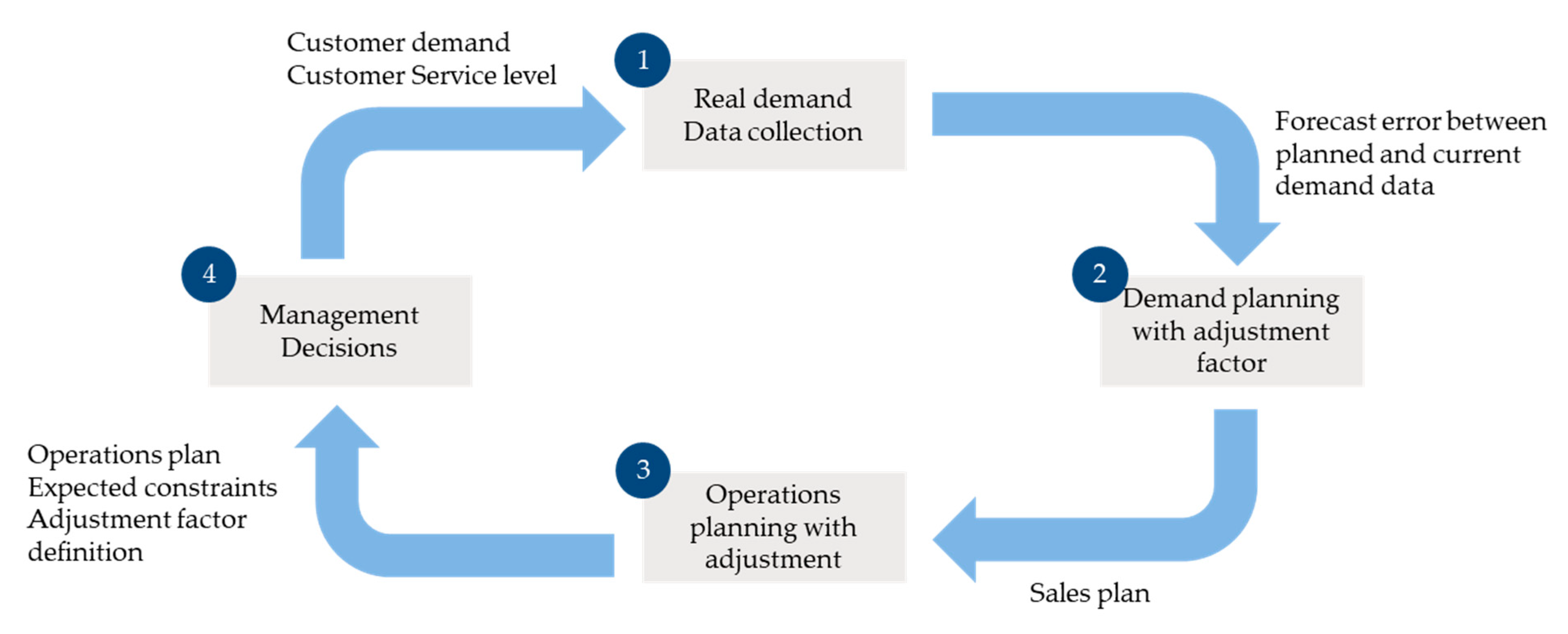
4.1.2. Development of the Conceptual Predictive Sales and Operations Planning Model

This model starts with the market. The manufacturer´s environment is the source of uncertainty and defines the potential events that will define the scenarios. Based on the potential events and their probabilities, the scenarios are derived. Normally, the areas related to strategy and marketing within organizations perform these kinds of activities. In the third step, forecasts of the future demand and sales plans are made, based on the given scenarios. Finally, operations plans are generated to level production over a certain planning horizon.

Given the framework in Figure 1, three main disturbances can be observed in practice, as illustrated in Figure 2:

A.

Alignment of sales planning with demand scenarios: Most companies enact sales plans based on forecasting methods. However, many of these plans are not related to, or do not consider, the potential scenarios. In addition, many of them do not monitor the current scenario in each planning period based on the events that have taken place.

B.

Solution preparation in the long term: What-if scenarios have certain implications in sales and operations plans. Theses implications can be predicted to define preventive measures for increasing efficiency by acting in advance to avoid undesirable planning consequences and results. In this context, many companies do not analyze in depth the potential implications of future scenarios or do not define what can be done to prevent these implications. Therefore, such companies are forced to take corrective measures to maintain system stability.

C.

Decisions in the medium term: Many companies know that certain events have taken place, and will identify potential planning actions to prevent inefficiency. However, many of these plans end with delayed decisions due to bureaucracy and discoordination, or end with suboptimal decisions due to organizational structures, such as silos, with divergent goals and interests.

Based on these three potential areas of improvement, a predictive methodological approach was developed. As shown in Figure 3, in the market environment, there are several potential scenarios with certain probabilities of occurring. Three scenarios are considered as this information is assumed on the simulation model. Then, based on the scenarios, the sales plan is generated and adjusted based on the expected and real demand values. Later, the operations plan is created by considering the supply chain, production, materials, and personal capacities and constraints. Finally, based on the expected results and past key performance indicators (KPIs), management decisions are analyzed to improve sales and operations planning performance aligned with the scenarios and the company´s strategy.

In Figure 3, the blue color indicates the given information for the simulation model, and the grey-colored boxes define the activities performed in the simulation model as the basis for the green-colored boxes, which define the potential decisions and the control limits for these decisions.

Figure 4 defines the steps of the predictive S&OP model. This model is divided into three different planning horizons: long-, medium-, and short-term. In the long term, a set of future events and scenarios is defined. The expected S&OP model can then be derived for each of the scenarios. Moreover, based on this predictive S&OP plan, impacts on the system efficiency can be identified. As a result, potential decisions and measures can be prepared as options for the future. These decisions are related to investments, working days or shifts, staff planning, and procurement and distribution partners. Decisions and their limits are defined based on predictive analysis in the long term.

In the medium term, preventive planning is generated based on a comparison of expected and real demand to detect deviations and decide whether to implement the options defined in the long-term scenario. In this time horizon, the supply chain system dynamics are analyzed, the similarities to the long-term scenarios can be identified, and the planning can be adjusted based on the deviations among the scenarios.

In the short term, measures are related to adjustments of the options prepared in the long term and implemented in the medium term. Unexpected events or a lack of preparation for expected events leads to corrective adjustments in the short term. These adjustments have a low impact on avoiding a decrease in system efficiency.

In

Table 1. Predictions to avoid corrections: from inefficiencies towards solutions within the supply chain.

No.	Areas	Expected Inefficiencies Detected within the Scenarios	Cause of the Inefficiency	Potential Solutions	Simulation Model Example
1	Procurement	1.1. Lack of Quantity 1.2. Lack of Quality 1.3. Delivery time or service level	1.1. Capacity 1.2. Time constraints/stress factor 1.3. Lead time	1.1. New contract for an increase in supplier´s capacity 1.2. Time horizon and specifications of procurement plans 1.3. Investment in consignment stock in producer´s plant	1.1. Supplier capacity expansion 1.2. Time horizon 1.3. Lead time due to new consignment stock
2	Production	2.1. Internal production capacity limitations 2.2. Personnel resources 2.3. Storage limitations 2.4. Lack of quality	2.1. Production capacities 2.2. Quantity, training, and /or motivation 2.3. Production lead time or storage capacities 2.4. Existing equipment, time constraints, or volume	2.1. Investments in new equipment, expanding existing capacities, or outsourcing production 2.2. Personnel acquisition, training, and leadership 2.3. Improvement of planning methodology, investments in new intermediate storage or expanding existing storage 2.4. New equipment, planning plans or volume leveling	2.1. Investment in expanding production capacities 2.2. Quantity of employees 2.3. Investment in expanding storage capacity 2.4. Volume leveling
3	Distribution	3.1. Delays and quantity received 3.2. Quality received 3.3. Storage problems leading to delays	3.1. Transport capacity or lead time to end-customers 3.2. Storage capacity and/or transport means 3.3. Storage capacity	3.1. New contract for capacity expansion or new distribution warehouses to reduce lead times 3.2. Investment in storage capacity or transport means 3.3. Expanding existing storage	3.1–3.3. New warehouse for reducing lead times

, the measures that can be implemented in the supply chain simulation model are described in relation to the expected inefficiencies.

As shown in Table 1, the predictive model within a supply chain seeks to detect potential inefficiencies within the given scenarios. Then, we can detect the cause of the inefficiency to determine the potential solutions. In this way, preparation of the solutions can be performed while allowing a shorter reaction time if the measure is intended to be implemented in the future. By following this sequence, any given supply chain within its areas of procurement, production, or distribution in any given set of scenarios can be modelled using system dynamics to identify the expected inefficiencies of the different scenarios, to perform a root-cause analysis, and to define the potential measures or solutions to treat the causes. By doing so, the future system stability is enhanced, and managers can make decisions based on the organizational strategy, goals, and current situation while understanding the future implications of engaging, or not engaging, in such decisions.

Given the different scenarios, a predictive demand plan for the planning intervals is derived. Based on this plan and the real demand collected after each period, the original demand plan is adjusted based on the average forecasted error between the planned and current demand. As a result, the operations plan can also be adjusted, and management decisions can be guided with the best available information. This planning loop is shown in Figure 5.

4.1.3. Definition of the S&OP Concept and Forecasting Techniques for Comparison

The S&OP concept for classical approaches is defined based on:

• Forecasts based on historical data;
• Sales plans based on forecasted values aggregated for a certain planning horizon;
• Operations plans defined by sales plans and the current system situation (the operations methods are the same as those for the predictive S&OP model);
• Demand pattern changes based on an analysis of historical data;
• The potential measures or investments to adapt capacities along the supply chain, which are not prepared or discussed with suppliers and/or distributors;
• The control limits for potential future decisions, which are not defined in advance.

The demand forecasting methods applied to the S&OP concept for the classical approach are the moving average, the mean of previous n values [40], and linear regression appropriate for stable trend [37]. In the model, the single moving average (SMA) with n equal to ten, and the cumulative moving average (CMA) with n as a variable, are applied, where D(t) is the demand of the item. In addition, in the linear regression, a is the slope of the trend, and $t_{trend}$ is the quantity of days since the trend demand pattern started, while b is the value when the demand pattern is initiated:

$$SMA=F_{\left(t+1\right)}=\frac{1}{n}{\displaystyle \sum }_{t=t-\left(n+1\right)}^t{D}_{\left(t\right)}$$

(1)

$$CMA= F_{\left(t+1\right)}=\frac{1}{n}{\displaystyle \sum }_{t=t-\left(n+1\right)}^t{D}_{\left(t\right)}$$

(2)

$$F_{\left(t+1\right)}=a · t_{trend}+b$$

(3)

The classical approach uses one of the previous methods to forecast customer demand. The classical simulation model can change between different forecasting methods depending on the demand pattern and an analysis of the historical data. Moreover, it can detect outliers, forecast sporadic trends, extend the moving average, and detect seasonal demands.

As in the predictive S&OP model, the classical simulation model prepares procurement, operations, and distribution plans based on the demand plan for the time horizon. Moreover, it can decide to invest in new capacities based on the expected gap between current capacities and future expected demand.

4.2. Statistical Treatment of Demand for a Defined Case Study

4.2.1. Demand Case Study

The model of the case study assumes information about the three scenarios and the series of data as given. When using forecasting for implementing a plan, it is recommended to consider different scenarios. Many studies refer to these different scenarios as base scenarios, high or low demand scenarios, higher or lower probability scenarios, or optimistic or pessimistic scenarios, among others. In this regard, the approach of the model is to process three different demand scenarios with their different probabilities of occurrence. These probabilities are set according to the case study. The time horizon for the simulation and, therefore, for the demand data is 1000 working days. The following values are the expected probability of occurrence for the different scenarios:

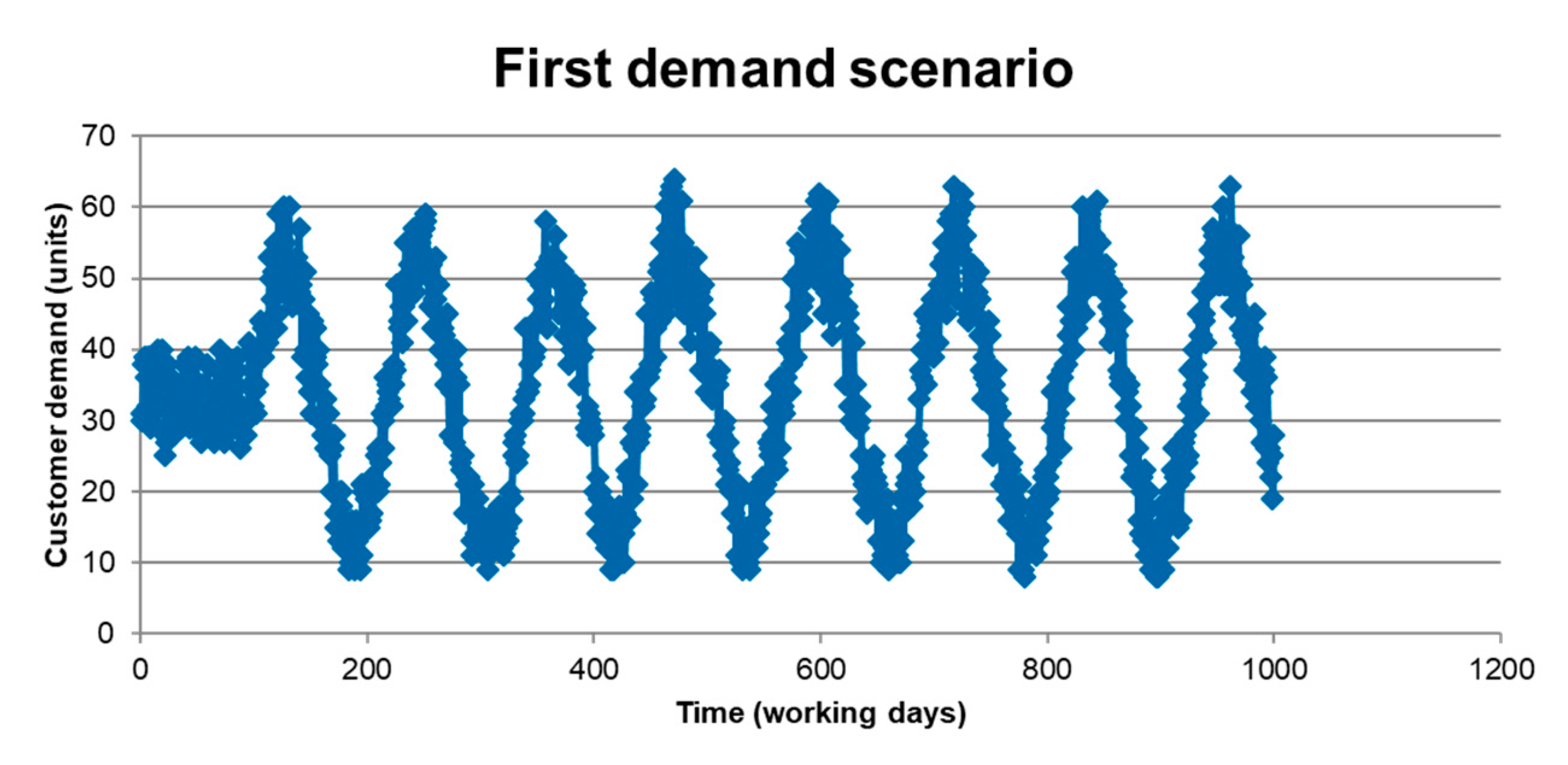
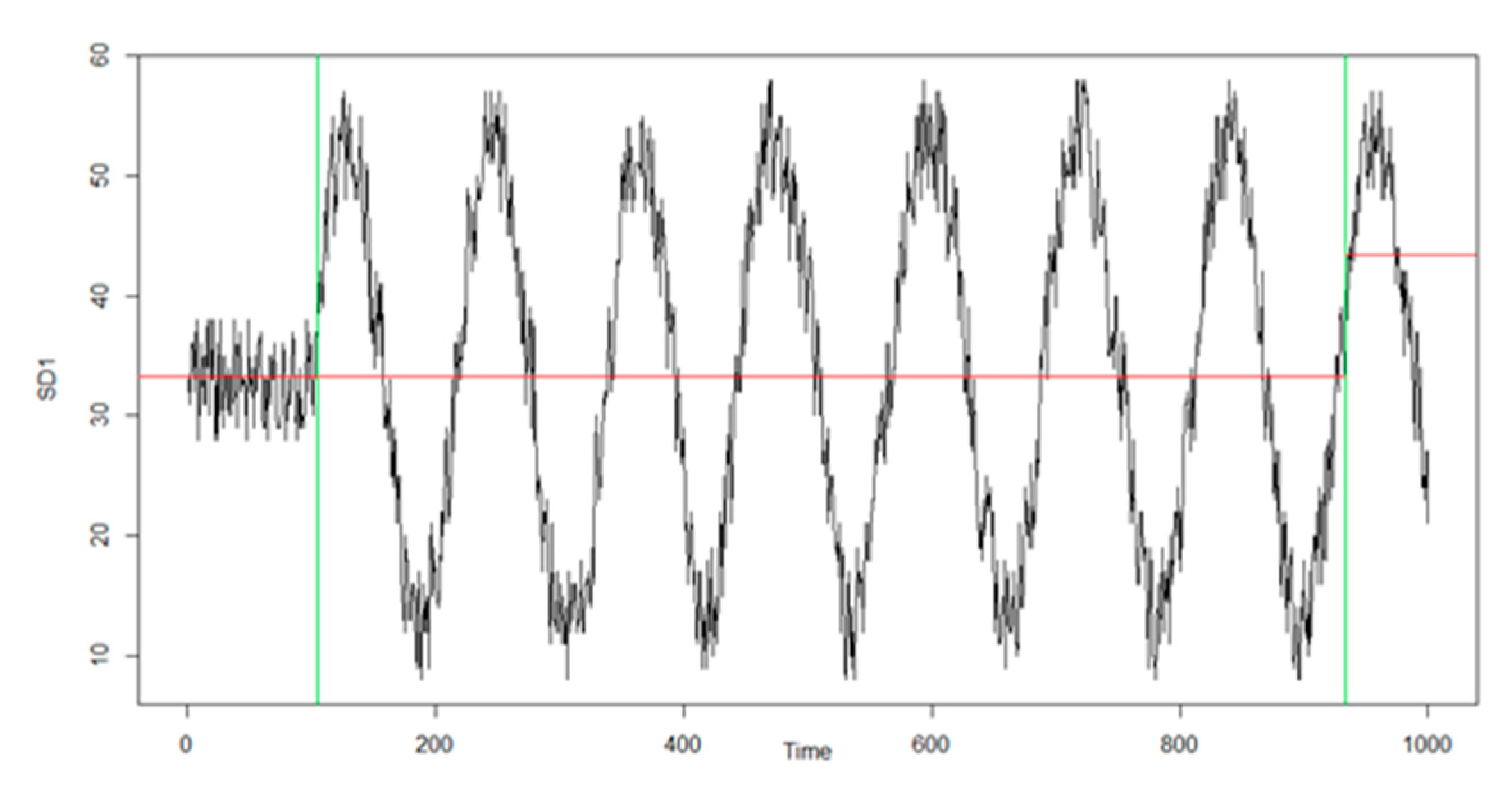
• The first demand scenario, or probable scenario, whose probability is 60%. As shown in Figure 6, it has an average demand value with a mean of 34 units ordered per day.

• The second demand scenario, or feasible scenario: 30% is the probability of occurrence for this scenario. As it can be seen in Figure 7, it has a minor decrease in average demand, compared to the first scenario, with a mean of around 32 units per day.

• The third demand scenario, or non-probable scenario: 10% is the probability of occurrence for this scenario. As it can be seen in Figure 8, it has more variability and a demand increase up to 39 units per day.

4.2.2. Statistical Treatment

The goal of this subsection is to apply the methodology with the following steps:

• Calculation of the expected demand based on the different scenarios and their probability of occurrence;
• Statistical analysis of the weighted expected demand (WED) to identify demand patterns and their changes;
• Generation of suitable random numbers.

First, the WED is calculated as the average of the three scenarios, with their different weights according to their probability of occurrence. Figure 9 shows the resulting demand data series.

Observing the time series helps to detect patterns or behaviors to obtain information about the series. In this research, a time series is characterized by a succession of data observed over time, obtained sequentially by default at regular intervals of time, in which the order of the data is important and cannot be altered. In this context, demand data fulfill these characteristics, as there is a demand value for each working day. To test if a data series is stationary, weak stationarity is chosen, in which a series is stationary if it is stable in its mean and autocovariance. A very useful function to measure the dependence between two separate h units of time is the autocorrelation function $\rho \left(h\right)=\gamma \left(h\right)/\gamma \left(0\right)$. The first step consists of observing the series (Figure 9) and determining its stationarity. For this purpose, the Dickey–Fuller test [41] (or unit roots) was applied using the R Studio test package [42], showing that the series is stationary because the p-value is < 0.05:

• Data: weighted expected demand (WED) data series;
• Test: augmented Dickey–Fuller test;
• Alternative hypothesis: stationary;
• Results:

  ○

  Dickey–Fuller = −3.7563;

  ○

  Lag order = 9;

  ○

  p-value = 0.02118.

Additionally, since approximately the first 100 data values present a lower variance than the rest of the data, a changepoint test was performed for the mean and variance using the changepoint package [43], the results of which are shown in

Table 2. Changepoints of the WED data series for the mean and variance.

No.	Changepoint Test Parameters	Mean	Variance
1	Changepoint Type	Change in mean	Change in variance
2	Test Statistics	Normal	Normal
3	Minimum Segment Length	1	2
4	Maximum no. of Changepoints	1	1
5	Changepoint Locations	933	105

. These results indicate a change in variance at point 105 and the average at 933.

In this way, the original time series can be decomposed into three time series: $S_1~\left({\mu }_1,{\sigma }_1^2\right)\in \left[1, 105\right]$, $S_2~\left({\mu }_1,{\sigma }_2^2\right)\in \left[106, 932\right]$, and $S_3~\left({\mu }_2,{\sigma }_2^2\right)\in \left[933, 1000\right]$. Since no additional information is available on the demand data series for the scenarios, the possible causes of these changes are not the goal of the research. Figure 10 shows the change points of the WED data series.

Based on the changepoint analysis, three different methods for random number generation were analyzed to select the one that best suits the WED data series:

A.

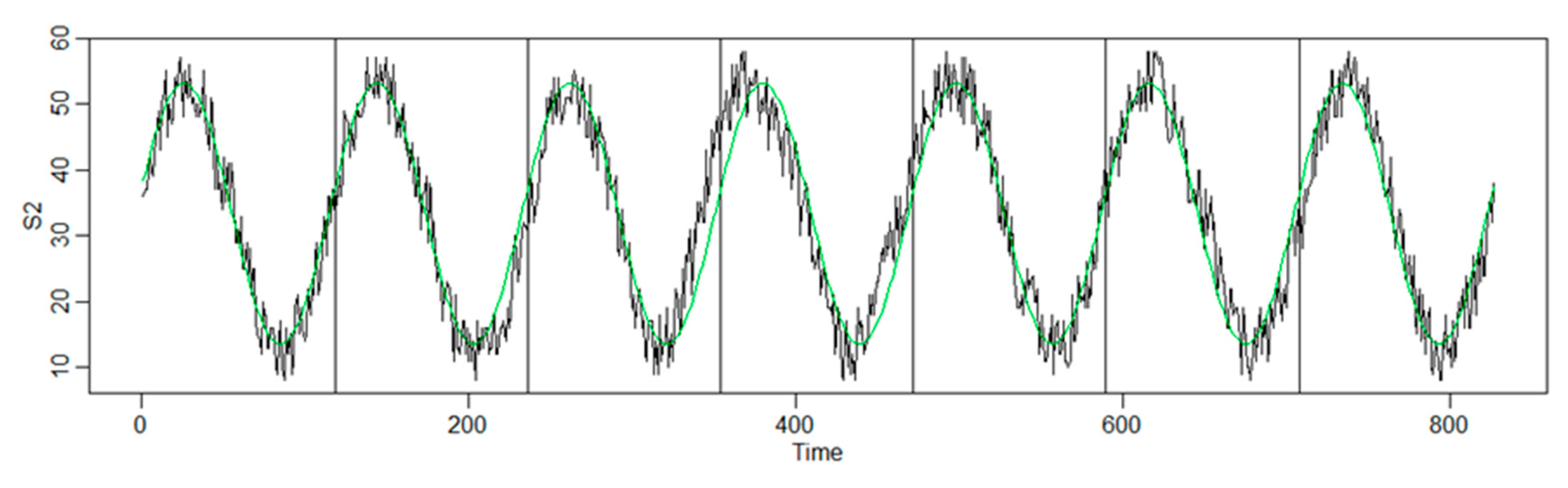
Harmonic series: A first approximation due to the periodic and cyclical nature of the series, which consists of carrying out a harmonic regression and a spectral analysis of the series, considering that each point of the series can be decomposed into a sum of sines and cosines, where $y_t$ is the value of the series at each time t, $a_j$ and $b_j$ are the j harmonic coefficients of the series, and n is the period of the series:

$$y_t=a_0+{\displaystyle \sum }_{j=1}^{\left(n-1\right)/2}\left[a_j\cos \left(2\pi t j/n\right)+b_j\sin \left(2\pi t j/n\right)\right].$$

(4)

Analysis of the S₂ data series provides a frequency of 0.008464 Hz, which indicates a period of 118.143 s—that is, the series is composed of a single wave that uses approximately 118 data values for one cycle. The coefficients a and b of the model are then estimated by harmonic regression, complemented by a study of higher order harmonics to determine their impact on the regression model.

Table 3. S₂ harmonic regression coefficients.

Coefficients	Estimates	p-Value
a0	33.3482	0.000
a1	3.9847	0.000
b1	19.3899	0.000
a2	0.2741	0.198
b2	−0.0055	0.979

shows the results of the following harmonic regression.

From the results, it is concluded that only a₀, a₁, and b₁ are significant (p-value < 0.05) unlike the higher order harmonics since their p-values are higher than 0.05. As a result, the residuals cannot be considered white noise, since there is a correlation between their values. Thus, the presumption of randomness here is not fulfilled, so the model is not adequate. This situation is explained by the fact that the period is not constant throughout the series, as reflected in Figure 11, which shows the adjusted series and the period compared to the original data.

B.

Autoregressive integrated moving average (ARIMA): An autoregressive model and moving averages of order p and q; ARIMA (p, q):

$$y_t={\phi }_1{y}_{t-1}+\dots + {\phi }_p{y}_{t-p}+a_t+{\theta }_1{a}_{t-1}+\dots + {\theta }_q{a}_{t-q}$$

(5)

where φ and θ are constants different from zero that show the weight of past observations and the errors in estimating future values of the series. By running the algorithm to determine the autoregression coefficients (auto.arima) in R Studio, an autoregressive (AR) (4) model, with four as the order p representing the number of previous values considered, can be obtained and its coefficients are shown in

Table 4. Autoregressive integrated moving average (ARIMA) correlation coefficients (4, 0, 0).

${\mathit{\phi }}_1$	${\mathit{\phi }}_2$	${\mathit{\phi }}_3$	${\mathit{\phi }}_4$	Mean
0.4743	0.2439	0.1682	0.0916	33.4616

.

The model is still not adequate since non-random behavior is observed among the model residuals, as shown in Figure 12.

C.

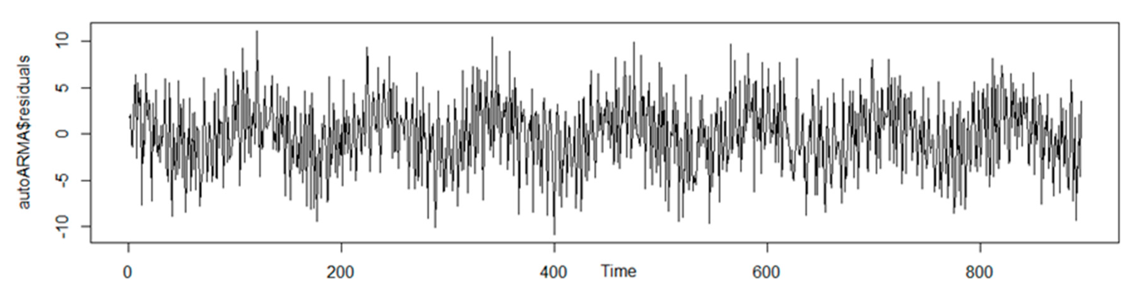
Artificial neural networks (ARNNs) (p, P, k) m: Autoregressive neural networks (ARNNs) are used to determine the most appropriate parameters for the model and if there is a model that better fits the data. Lapedes and Farber [44] were the first to use a neural network for prediction purposes by applying a feedforward multilayer network. The autoregressive neural network model ARNN (p, P, k) m is equivalent to an ARIMA model (p, 0, 0) (P, 0, 0)m, where m is the seasonal component of the series, and k is the number of neurons in the hidden layer. The result achieved is an ARNN (25, 13, 1), which translates into an AR (25) with a component 13 to ensure seasonality, and a neuron is used in the hidden layer, which is equivalent to an ARIMA (25, 0, 0) (13, 0, 0)₁. Likewise, a normality test is performed to determine if this layer corresponds to Gaussian noise (Shapiro–Wilks test (p-value = 0.7856) at ~N (0, 2.71)). This methodology confirms the results initially collected in the ACF (Auto Correlation function) and PACF (Partial Auto Correlation function) correlograms. Likewise, the absence of autocorrelations and dependence of the residuals are confirmed through the ACF correlogram in Figure 13, which is why it is concluded that this layer is Gaussian white noise:

The model presents 25 correlation coefficients and a mean for the calculations. The greater complexity of the model compensates for the lower errors in the model and the Gaussian white noise in the residuals.

Table 5. Prediction extracts and their confidence intervals at 80% and 95%.

Prediction Value	CI 80%		CI 95%
19,443	17,518	21,531	16,540	22,681
18,742	16,640	21,011	15,499	22,438
18,286	16,382	20,569	15,330	21,549
20,452	18,316	22,698	17,155	24,060
15,472	13,965	17,491	13,127	18,459
20,954	18,413	23,265	17,306	25,200

shows the predictions of the values (13) and the confidence intervals (CI) for 80% and 95% of the predictions.

4.2.3. Random Number Generation for Future Expected Demand

Based on the statistical treatment, there are three different demand patterns involving three states over the four years of the simulation model. In this context, the generation of random numbers for the expected demand is performed, following the functions and characteristics shown in

Table 6. Demand patterns, periods, and methods for random number generation.

No.	Demand Pattern	Period	Parameters	Method or Formula for Demand Data Generation
1	$S_1,$Stationary	1–105	Mean	Mean with random numbers between (−2$\sigma$, 2$\sigma$)
2	$S_2,$Cyclical 1	106–932	ARIMA	ARIMA value + noise
3	$S_3,$Cyclical 2	933–1000	ARIMA	ARIMA value + noise

:

Random number generation is performed for the next twelve working days for each working day of the simulation period. This means that on day 102, demand values are generated for the days from day 103 to day 114.

4.3. Simulation Case Study

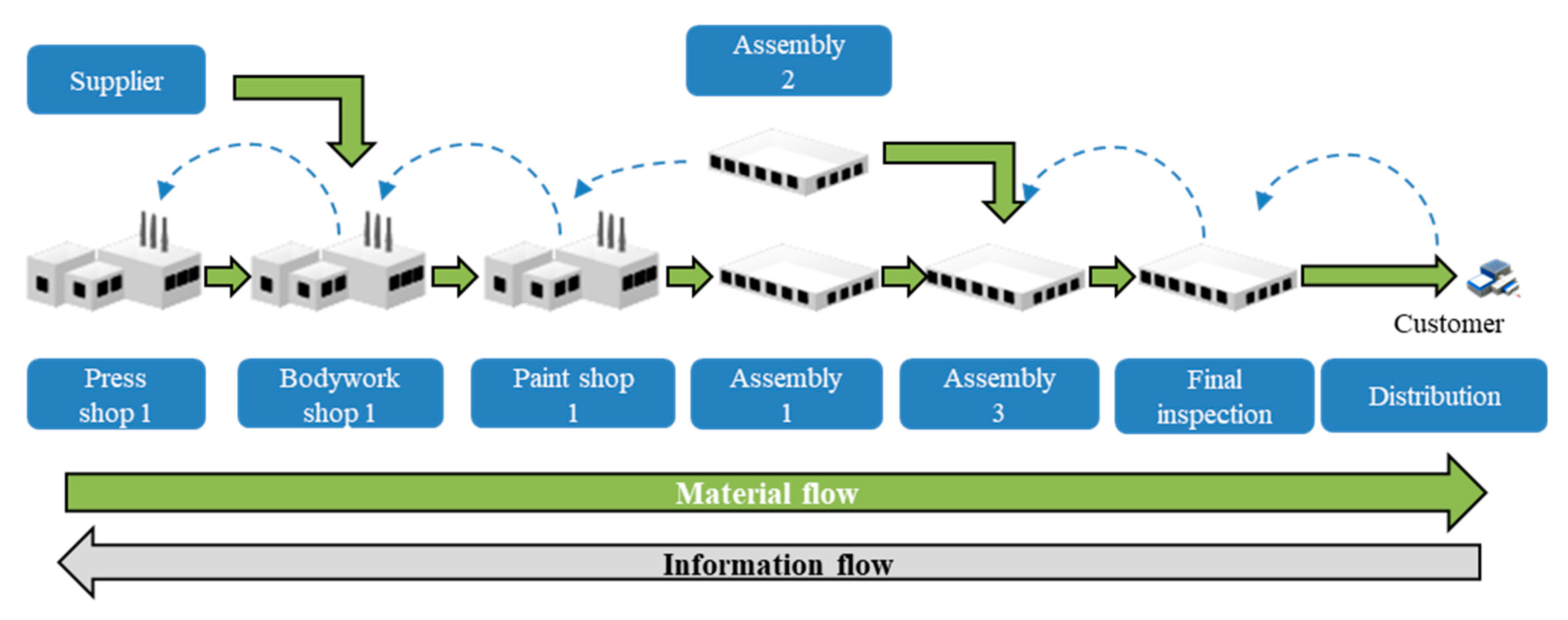
4.3.1. Design of the Supply Chain Flow and Planning Characteristics for a Manufacturer

The supply chain system consists of a process that begins with steel stamping and ends with the distribution of the manufactured cars to end-customers. The supplier, manufacturer production shops, and distribution within the supply chain flow are shown in Figure 14 and listed below. The capacity values refer to the nominal values for three working shifts at the beginning of the simulation model:

○

Supplier: A nominal capacity of 40 units per day. It delivers pressed pieces to the bodywork shop of the manufacturer;

○

Press, bodywork, paint, pre-assembly or assembly 1, mechanical assembly shop or assembly 2, final assembly or assembly 3, and the final inspection shops: All of these shops have a nominal capacity of 36 units per day;

○

Distributor: Has a nominal capacity of 40 units per day.

Both models, the classical approach and the predictive S&OP model, present the same supply chain flow. Moreover, their planning characteristics are as follows:

○

Order backlog: At the beginning of the simulation, the model has a certain level of WIP units. In addition, the model presents ordered and undelivered car units at the beginning of the simulation. This value relates to 1320 car units ordered and waiting to be delivered to end-customers.

○

Release of orders: The initiation of orders is controlled before production at press shop 1. This shop controls the number of orders that enter the production process. After the initiation of the production process, the planning logic is a push-strategy until reaching the end-customer. The release of orders depends on the order backlog, the customer order lead time, the nominal capacity of press shop 1, and the demand forecast. This process depends on the same four parameters for both models; however, the values of the parameters vary between both.

○

Demand forecasting: Both models forecast future demands at different planning horizons. Both models forecast future demand values. However, the methods for determining these values vary. The predictive S&OP model uses the generated random numbers with the adjustment factor, while the classical approaches calculate the demand forecast based on formulas according to historical data.

○

Demand planning: The same process for the aggregation of demand at different planning horizons. Long-term demand planning is calculated for one year, medium-term demand planning is performed for one month and three months, and short-term demand planning is obtained on a daily basis.

○

Production planning: As mentioned in the order release section, the production planning strategy seeks to control the order release to ensure that the WIP units are sufficient to meet the promised customer order lead time and the promised weekly delivery goals. In this context, after production initiation, the logic involves a push-production strategy with intermediate stock between the production shops. As a result, the production output in each shop aims to be as large as possible. However, if demand is not high, the model ensures that the WIP units are not too numerous at the end of the supply chain process without a customer order. This model, therefore, seeks to avoid make-to-stock production while favoring make-to-order production—orders placed by the customer, and not internal or dealer orders. Therefore, in cyclical demands, there are periods with mid–low utilization of production capacities, with high utilization employed in other planning periods.

○

Personal planning: both models use demand plans to determine the number of employees that require a planning period. Moreover, the flexibility of the employees can increase or decrease the capacity of shops by six units per day. Based on the production requirements, the system decides whether to increase the quantity of employees or to reduce it. As a result, operational expenses or savings can be obtained.

○

Procurement planning: Both models receive procurement plans from the manufacturer based on the demand forecast.

○

Distribution planning: Both models receive distribution plans from the manufacturer based on the WIP units following a push-strategy.

○

Investment planning: Both models have the capability to decide upon new investments for new capacities at the supplier, the manufacturer, and the distributor level. However, the parameters and implementation time are different. The predictive S&OP model assesses the investment based on the control limits derived from the root cause analysis and preparation of solutions.

As indicated in Table 1, the options for the predictive S&OP model are shown in the right column. These options represent the main difference between the two models in comparison. The predictive S&OP model is able to prepare management decisions and their implementations to respond to future potential inefficiencies. By doing so, control limits can be defined. This allows the model to decide on management changes and their implementation efficiently whether if it is:

○

For procurement management due to preagreements between supply chain parties:

• Supplier capacity expansion.
• Reduction of replenishment lead time due to a new warehouse or due to a new consignment stock due.

○

For production management due to internal decision-making committees:

• Expanding production capacities.
• Changes in the quantity of employees.
• Expanding storage capacity.
• Changes in planning method and parameters for volume leveling.

○

For distribution management due to preagreements between supply chain parties:

• New warehouse for reducing distribution lead times.

In this context,

Table 7. Simulation logic differences between models (own elaboration).

No.	Area	Classical S&OP Model	Predictive S&OP Model
1	Demand scenarios	No treatment.	Statistical treatment for the identification of demand patterns, expected demand changes, and generation of random numbers. Use of statistical software and datasheets in Excel.
2	Forecasting techniques	SMA, CMA, linear regression. Selection based on historical data analysis for demand pattern identification.	Based on random number generation. Adjustment of the random number generation based on the forecast error between planned and current demand data, as shown in Figure 5.
3	Sales plan	Based on the forecast for the planning horizons.	Generation of an original demand plan based on statistical treatment. Adjustment of the original demand plan based on a planned/actual comparison for the planning horizons.
4	Procurement, production, distribution and personal plans	Based on the classical S&OP model sales plan, the subsequent plans are derived.	Based on the predictive S&OP model sales plan, the subsequent plans are derived. Plans and their methods can change based on the management decisions preparation.
5	Investment planning	Decisions and limits for initiating a measure are not defined. As a result, the implementation time is longer.	Investment assessed based on the control limits derived from the root cause analysis and preparation of solutions. As a result, the implementation time is shorter.

shows the main differences in the simulation logic of both models:

4.3.2. Assumptions and Restrictions

The following restrictions were defined, and several assumptions were made. These restrictions and assumptions are the same for both models, unless otherwise specified:

• Time restrictions: As this model considers from long-term to short-term horizons, four working years are simulated to evaluate influences in the short, medium, and long term. Assuming 250 working days per year, 1000 time periods are simulated.
• The existing product is in a mature stage of its lifecycle, with stable demand of 33 units per day in the first working days of the simulation.
• Production capacity has a nominal capacity of 36 units per day in three shifts at the beginning of the simulation for the manufacturer process, and 40 units per day for supplier and distribution. As a consequence, the model at initial time is able to supply, produce, and distribute based on the stable demand of 33 units per day, given a stable model at the beginning:

  ○

  During the simulation, two investment options for the manufacturer shops are considered: an increase of 9 units per day or an increase of 18 units per day.

  ○

  Two other investment options are also analyzed. These include capacity increases of 20 units per day for the supplier and distributor.

• Customer demand is read from Excel files.
• Volume loss depends on the customer demand level and the customer order lead time.
• Random numbers for future demand are read from Excel files.
• The simulation model considers sales losses starting from a customer order lead time greater than 60 days.
• The bodywork shop is assumed to need one unit of the supplier and one unit of press shop 1 to produce the body of the car.
• The order backlog is the same for both models at the beginning of the simulation.
• A car is a finished product after it initiates the distribution following the final inspection shop.
• The warehouses have no stock capacity limitations. It is assumed that outsourcing warehouses for stocks can be found nearby with extra-holding costs.
• There is no transport limitation between the different production stages. It is assumed that additional third-party logistics can be found.
• There is a limitation in production capacities and distribution capacities.
• A steady supply of materials for the press shop of the car manufacturer is provided.
• The available number of products is known at every moment of the production, inventory, and transport processes.
• This is a low volume automotive manufacturer, for which customer orders are not changeable.
• Order information along the supply chain is available.
• Data on historical demand are available for both models one day after the demand.

4.3.3. Demand Scenarios and Simulation Models

There are three demand scenarios, as explained in Section 4.2.1:

• First demand scenario or probable scenario.
• Second demand scenario or feasible scenario.
• Third demand scenario or non-probable scenario.
• There are two simulation models for comparison of the results:
• Predictive S&OP simulation model.
• Classical S&OP simulation model.

These two simulation models correspond to the characteristics defined in Section 4.1.2 and Section 4.1.3, respectively.

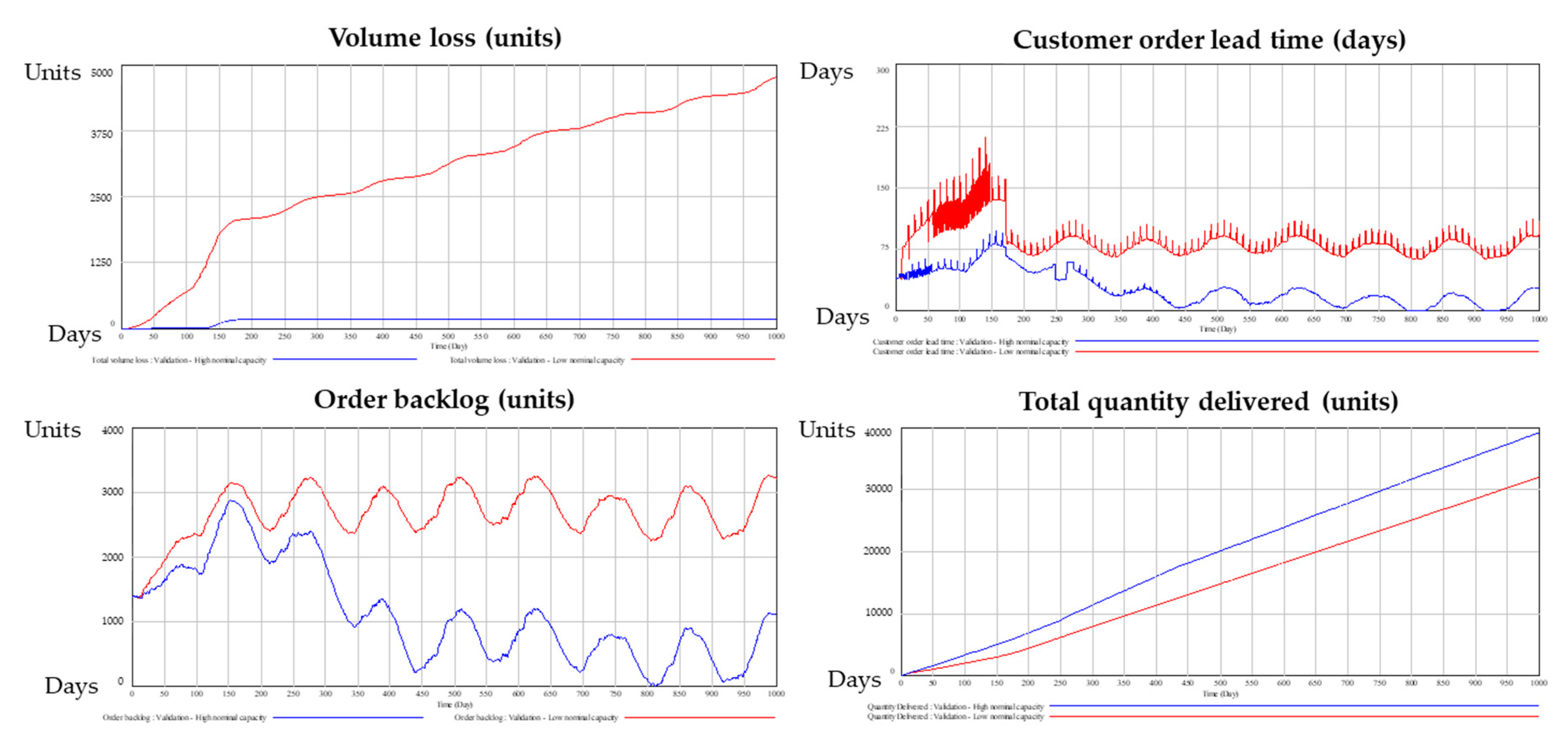
4.3.4. Simulation Model Validation

Before obtaining the results of the scenarios for both simulation models, validation was performed for both. An extreme-value test was chosen as one of the 12 possible methods for validating the relevant system dynamics models [45]. For both models, the same input and output variables were chosen to analyze and validate the models. These parameters are the nominal capacity and the customer demand. Based on the changes of values among these factors, the following results are expected to be logical and conclude the validation:

• For a lower nominal capacity (units per day), the customer order lead time, volume loss, and order backlog must be higher, and the total quantity delivered must be lower, as shown in Figure 15.
• For a lower customer demand (units per day), the customer order lead time, volume loss, and order backlog are lower, and the total quantity delivered must also be lower.

These two extreme-value tests were validated for both models successfully.

4.4. Simulation Results for the Case Study of an Automotive Plant

After the validation, the results for the three demand scenarios were extracted for the selected key performance indicators.

In the first potential scenario, the predictive S&OP simulation model produces better results for all relevant indicators, as shown in

Table 8. Simulation results for demand scenario 1 (probable scenario).

No.	Key Performance Indicator (KPI)	Classical S&OP Simulation Model	Predictive S&OP Simulation Model
1	Cumulated potential demand (units)	34,062	34,062
2	Cumulated demand (units)	32,742	34,030
3	Cumulated volume loss (units)	1320	32
4	Cumulated quantity delivered (units)	32,154	34,478
5	Average quantity delivered on-time per week (%)	77.3	95.9
6	Average WIP stock (units)	4374	278
7	Average capacity utilization of the production plant (%)	71.0	66.8
8	Average customer order lead time (days)	65.0	28.7
9	Average mean absolute deviation (MAD) per week (units)	28.5	17.0
10	Average order backlog (units)	1847	971
11	Cumulated operational savings (M euros)	0.1	0.8
12	Cumulated investment value (M euros)	14.7	14.4

, except for the average capacity utilization. However, this model’s capacity utilization level is lower, due to the greater prior increase in capacity, compared to the classical S&OP model. Among these parameters, it is important to point out five characteristics:

• The volume loss of 32 units versus 1320 units in the classical approach. This means that the predictive model can adapt itself to demand needs by not allowing the loss of customers and the associated orders.
• The total quantity delivered is more than 2000 additional units over the simulation period. Moreover, the quantity delivered on time is almost 20% higher than that in the classical approach. This means that the model can fulfill its commitments in terms of delivery quantity and date. As a result, the planning stability of this model in this scenario is higher than that in the classical S&OP model.
• The WIP stock along the manufacturer´s production process is almost 20 times lower for the predictive S&OP model, as it is able to regulate production and stocks by predicting the cyclical demand patterns.
• The customer order lead time is more than two times lower in the predictive S&OP model aligned with almost half of the average order backlog.
• The operational savings in the predictive S&OP model are higher due to this model’s ability to plan personal resources based on future demand needs.

Therefore, similar to the first scenario, based on a comparison of the models, the results show that the predictive S&OP simulation model would be desirable in this demand scenario, due to its combination of a highly-efficient lead time, on-time delivery, and WIP stock, while also securing the potential customer demand with higher operational savings and the same level of investments as that of the classical S&OP approach.

In the second potential scenario, the predictive S&OP simulation model produced better results for all relevant indicators, as shown in

Table 9. Simulation results for demand scenario 2, the feasible scenario.

No.	Key Performance Indicator (KPI)	Classical S&OP Simulation Model	Predictive S&OP Simulation Model
1	Cumulated potential demand (units)	32,174	32,174
2	Cumulated demand (units)	31,202	32,064
3	Cumulated volume loss (units)	972	110
4	Cumulated quantity delivered (units)	30,948	32,445
5	Average quantity delivered on-time per week (%)	76.6	95.3
6	Average WIP stock (units)	4159	267
7	Average capacity utilization of the production plant (%)	68.9	71.7
8	Average customer order lead time (days)	59.7	32.8
9	Average mean absolute deviation (MAD) per week (units)	31.5	20.0
10	Average order backlog (units)	1602	1004
11	Cumulated operational savings (M euros)	0.2	0.7
12	Cumulated investment value (M euros)	14.7	5.7

. In addition, two different trends can be outlined, in comparison to scenario 1:

• The capacity utilization level is higher for the predictive S&OP model because the investment in new capacities is 5.7, while for the classical S&OP model, this value is 14.7 million euros. This difference occurs because the predictive S&OP model is able to determine that no more capacity is needed to secure delivery on time (95.3%), and a delivery quantity of almost 1500 units more than the classical model can be secured.
• As the customer demand in this scenario is lower, and the predictive S&OP model optimizes resources and investments, the difference between the two models is not as high as that under the first demand scenario.

Finally, as in the first scenario, based on a comparison of the models, the results show that the predictive S&OP simulation model is most desirable in this demand scenario, due to its combination of a highly-efficient lead time, on-time delivery, and WIP stock, while also securing potential customer demand with higher operational savings and a lower level of investments, compared to the classical S&OP approach.

As explained for scenarios 1 and 2, similar results were obtained for the third scenario as it shows

Table 10. Simulation results for demand scenario 3, the non-probable scenario.

No.	Key Performance Indicator (KPI)	Classical S&OP Simulation Model	Predictive S&OP Simulation Model
1	Cumulated potential demand (units)	39,090	39,090
2	Cumulated demand (units)	34,780	38,959
3	Cumulated volume loss (units)	4310	131
4	Cumulated quantity delivered (units)	32,986	38,863
5	Average quantity delivered on-time per week (%)	75.6	97.0
6	Average WIP stock (units)	5512	350
7	Average capacity utilization of the production plant (%)	70.6	70.3
8	Average customer order lead time (days)	92.9	34.1
9	Average mean absolute deviation (MAD) per week (units)	78.5	66.0
10	Average order backlog (units)	2528	1327
11	Cumulated operational savings (M euros)	0.0	0.9
12	Cumulated investment value (M euros)	20.1	14.4

. However, there are two relevant facts:

• In this scenario, the supply chain system is under stress due to cyclical demand with a high average; the predictive S&OP model is, however, able to achieve 97.0% on-time delivery while maintaining low stock levels, customer order lead times, and securing potential demand with only 131 car orders lost. This model also yields lower investments by almost six million euros alongside almost one million euros in operational savings compared to the classical S&OP model.
• As the customer demand in this scenario is higher than that in the previous two scenarios, and the predictive S&OP model optimizes resources and investments, the differences between the two models are greater than those under other scenarios.

Therefore, based on a comparison of the models, the results show that the predictive S&OP simulation model is most desirable among the three demand scenarios due to its higher efficiency in terms of customer service level, planning stability, investments, and operational savings. The key factor for these results is the ability to predict potential inefficiencies to prevent them from happening by applying measures before the short term, at which point only corrective measures can be applied. Another key factor is that the forecast error, measured with the MAD, is much lower for the predictive S&OP model under all three scenarios. This provides adequate planning stability to detect deviations, identify effective measures, and determine the best fit to decide and implement the relevant solutions to maintain and boost the supply chain system’s efficiency.

Finally, a comparison of the factors among the three simulation scenarios was performed, as shown in

Table 11. Comparison of simulation results for the predictive S&OP models between scenarios and factors.

No.	Key Performance Indicator (KPI)	Scenario 1—Probable	Scenario 2—Feasible	Scenario 3—Non-Probable
1	Cumulated potential demand (units)	Middle	Low	High
2	Cumulated demand (units)	Middle	Low	High
3	Cumulated volume loss (units)	Low	Middle	High
4	Cumulated quantity delivered (units)	Middle	Low	High
5	Average quantity delivered on-time per week (%)	Middle	Low	High
6	Average WIP stock (units)	Middle	Low	High
7	Average capacity utilization of the production plant (%)	Low	High	Middle
8	Average customer order lead time (days)	Low	Middle	High
9	Average mean absolute deviation (MAD) per week (units)	Low	Middle	High
10	Average order backlog (units)	Low	Middle	High
11	Cumulated operational savings (Mill. Euros)	Middle	Low	High
12	Cumulated investment value (M euros)	Middle	Low	Middle

. This table compares the scenarios by classifying them as low, middle, or high value in comparison with the other two scenarios.

Scenario 1 has a middle demand level and middle values for many of the factors. On the other hand, as the demand uncertainty is lower here than in scenario 2, the volume loss is lower, the lead time is shorter, and the order backlog is lower. Moreover, as the scenario invests at the same level as scenario 3, its capacity utilization is the lowest among the three scenarios.

Scenario 2 has the lowest demand and, therefore, the lowest quantity delivered, the lowest stock units, and the lowest investments and operational savings. However, it presents a higher MAD than scenario 1, and, as a consequence, it loses greater volume and has a longer customer order lead time and a larger order backlog than scenario 1.

Scenario 3 presents the highest factor values for all parameters, excluding the capacity utilization of the production plant. This can be explained by the increase in capacity due to investments. With investments at the same level as those in scenario 1, the utilization of capacities is higher.

5. Conclusions

As a result of this research, the main hypothesis was supported based on the following observations:

• Using the new conceptual model for sales and operational planning, based on a statistical treatment of customer demand, planning stability and accuracy can be improved.
• The predictive S&OP model is able to predict potential inefficiencies, define causes, determine effective measures, and implement solutions, thus increasing the efficiency of resource utilization within a supply chain and securing the long-term viability of manufacturers.
• The predictive S&OP model enables manufacturers to improve their service levels, thus securing their entire potential customer demand.
• The abovementioned points demonstrate the need for such a system as a standard tool for managers in the future to increase the efficiency and adaptability of manufacturing organizations by following the principle of “predicting to define preventive measures to avoid correcting”.
• System dynamics provides the necessary platform to determine the cause–effect parametrization and thus obtain results relevant to the research purpose.
• The simulation of an automotive supply chain using the developed conceptual model offers better results than those obtained using currently-available S&OP approaches for dealing with different demand scenarios.

The contributions of this paper can be summarized under three areas: theoretical, managerial, and empirical. In this section, the limitations of the study and potential future research are also described.

Theoretical conclusions:

• A description of current research challenges related to sales and operations planning;
• The design of a generic predictive methodology to optimize sales and operations planning: This developed methodology combines demand scenarios, a statistical analysis of demand, forecasting techniques, random number generation, and system dynamics;
• The development of a simulation model that applies system dynamics to evaluate the impact of the developed predictive approach.

Managerial conclusions:

• The description of current practical challenges related to sales and operations planning;
• A predictive approach to identify planning challenges, prepare solutions, and implement these factors accordingly was proven to be key for increasing the competitiveness of organizations;
• This predictive model can serve as a fundamental tool for managers, especially for those facing uncertain situations with different potential demand scenarios and future events.

Empirical conclusions: To prove the effectiveness of the developed methodology, a statistical treatment of potential scenarios and a simulation of the supply chain of an automotive producer were employed. Classical and predictive S&OP models were implemented in the Vensim software and simulated to compare the performance under three demand scenarios. The benefits of changing from a classical S&OP approach to an approach using a predictive S&OP approach are as follows:

• Better customer service level.
• Lower customer order lead time.
• Higher planning stability.
• Lower stock level.
• Lower volume loss.
• Lower investments and higher operational savings.

Limitations of the research work:

• The methodology and simulation model were not proven in any organization.
• The complexity of the supply chain was partially built into the simulation model using the assumptions set.
• The organization structure, S&OP meetings, and interfaces between organizational areas were not considered in the simulation model.
• Information along the supply chain was assumed to be available.

In future potential research, we may analyze how to transform this model into a tool able to assist managers by simulating what-if scenarios to identify inefficiencies and provide suggestions for potential solutions in order to improve the competitiveness of manufacturing organizations.

References

- Schuh, G.; Stich, V.; Wienholdt, H. Logistikmanagement; Springer: Berlin/Heidelberg, Germany, 2013. [Google Scholar]
- Frazelle, E. Supply Chain Strategy: The Logistics of Supply Chain Management; McGraw Hill: New York, NY, USA, 2002; p. 117. [Google Scholar]
- Siller, U. Optimierung Globaler Distributionsnetzwerke: Grundlagen, Methodik, Praktische Anwendung; Gabler Verlag: Wiesbaden, Germany, 2011. [Google Scholar]
- Christopher, M. Logistics and Supply Chain Management; Logistics and Supply Chain Management Creating Value-Added Networks; Pearson Education Limited: Great Britain, UK, 2005. [Google Scholar]
- Wildemann, H. Entwicklungspfade der logistik. In Das Beste Der Logistik; Springer: Berlin/Heidelberg, Germany, 2008; pp. 161–172. [Google Scholar]
- Christopher, M. Logistics & Supply Chain Management Pearson Education; Pearson Education Limited: Harlow, UK, 2011. [Google Scholar]
- Jodlbauer, H. Produktionsoptimierung; Springer Science & Business: Berlin, Germany, 2008. [Google Scholar]
- Placzek, T.S. Optimal Shelf Availability: Analyse und Gestaltung Integrativer Logistikkonzepte in Konsumgüter-Supply Chains; Springer: Wiesbaden, Germany, 2007. [Google Scholar]
- Capgemini. Customer Back on Top of the Supply Chain Agenda in 2010. from Financial Crisis to Recovery: Does the Financial Crisis Still Dictate Supply Chain Agendas? Capgemini Consulting: Utrecht, The Netherlands, 2010. [Google Scholar]
- McKinsey. McKinsey: McKinsey on Supply Chain; Select Publications: Chicago, IL, USA, 2011. [Google Scholar]
- Sydow, J. Management von Netzwerkorganisationen–Zum stand der forschung. In Management von Netzwerkorganisationen; Springer: Berlin/Heidelberg, Germany, 2010; pp. 373–470. [Google Scholar]
- Ijioui, R.; Emmerich, H.; Ceyp, M.; Diercks, W. Supply chain event management als strategisches unternehmensführungskonzept. In Supply Chain Event Management: Konzepte, Prozesse, Erfolgsfaktoren Und Praxisbeispiele; Physica-Verlag: Berlin/Heidelberg, Germany, 2007; pp. 3–14. [Google Scholar]
- Bundesverband Logistik BVL. Studie Trends und Strategien in der Logistik 2008: Die Kernaussagen; Frank straube und hans-christian pfhol; Deutscher Verkehrs-Verlag: Bremen, Germany, 2008. [Google Scholar]
- Schikora, A. Anforderungen an Die Unternehmensführung im Turbulenten umfeld; Igel Verlag RWS: Hamburg, Germany, 2005. [Google Scholar]
- Pfohl, H. Logistiksysteme: Betriebswirtschaftliche Grundlagen; Springer: Berlin/Heidelberg, Germany, 2004. [Google Scholar]
- Wiendahl, H. Auftragsmanagement der Industriellen Produktion: Grundlagen, Konfiguration, Einführung; Springer: Berlin/Heidelberg, Germany, 2011. [Google Scholar]
- Meier, C. Echtzeitfähige Produktionsplanung und-Regelung in der Auftragsabwicklung des Maschinen-und Anlagenbaus; Apprimus-Verlag: Aachen, Germany, 2013. [Google Scholar]
- Fleisch, E.; Christ, O.; Dierkes, M. Die betriebswirtschaftliche vision des internets der dinge. In Das Internet Der Dinge; Springer: Berlin/Heidelberg, Germany, 2005; pp. 3–37. [Google Scholar]
- Hellmich, K.P. Kundenorientierte Auftragsabwicklung: Engpassorientierte Planung und Steuerung des Ressourceneinsatzes; Springer: Berlin/Heidelberg, Germany, 2003. [Google Scholar]
- Fischäder, H. Störungsmanagement in Netzwerkförmigen Produktionssystemen; Springer: Berlin/Heidelberg, Germany, 2007. [Google Scholar]
- Otto, A. Supply chain event management: Three perspectives. Int. J. Logist. Manag. 2003, 14, 1–13. [Google Scholar] [CrossRef]
- Kristensen, J.; Jonsson, P. Context-based sales and operations planning (S&OP) research. Int. J. Phys. Distrib. Logist. Manag. 2018, 48, 19–46. [Google Scholar]
- Ambrose, S.C.; Rutherford, B.N. Sales and Operations Planning (S&OP): A Group Effectiveness Approach. Acad. Market. Stud. J. 2016, 20. Available online: https://commons.erau.edu/publication/1121/ (accessed on 28 December 2020).
- Manikas, A.; Godfrey, M.; Skiver, R. Using Big Data to Predict Consumer Responses to Promotional Discounts as Part of Sales & Operations Planning. Int. J. Manag. Mark. Res. 2017, 10, 69–78. [Google Scholar]
- Dubey, R.; Gunasekaran, A.; Childe, S.J.; Blome, C.; Papadopoulos, T. Big data and predictive analytics and manufacturing performance: Integrating institutional theory, resource-based view and big data culture. Br. J. Manag. 2019, 30, 341–361. [Google Scholar] [CrossRef]
- Ylijoki, O. Guidelines for assessing the value of a predictive algorithm: A case study. J. Mark. Anal. 2018, 6, 19–26. [Google Scholar] [CrossRef]
- Kühnapfel, J.B. Vertriebsprognosen. In Vertriebscontrolling; Springer Gabler: Wiesbaden, Germany, 2014. [Google Scholar]
- Stadtler, H.; Kilger, C. Supply Chain Management and Advanced Planning; Springer: Berlin/Heidelberg, Germany, 2005; Volume 3. [Google Scholar]
- Campuzano, F.; Mula, J. Supply Chain Simulation: A System Dynamics Approach for Improving Performance; Springer Science & Business Media: Berlin, Germany, 2011; p. 23. [Google Scholar]
- Meisel, M.; Leber, T.; Ornetzeder, M.; Stachura, M.; Schiffleitner, A.; Kienesberger, G.; Wenninger, J.; Kupzog, F. Smart demand response scenarios. In Proceedings of the IEEE Africon ’11, Livingstone, Zambia, 13–15 September 2011; IEEE: New York, NY, USA, 2011; pp. 1–6. [Google Scholar]
- Suryani, E.; Chou, S.Y.; Hartono, R.; Chen, C.H. Demand scenario analysis and planned capacity expansion: A system dynamics framework. Simul. Model. Pract. Theory 2010, 18, 732–751. [Google Scholar] [CrossRef]
- Thupeng, W.M.; Thekiso, T.B. Changepoint analysis: A practical tool for detecting abrupt changes in rainfall and identifying periods of historical droughts: A case study of botswana. Bull. Math. Stat. Res. 2019, 7, 33–46. [Google Scholar]
- Jewell, S.; Fearnhead, P.; Witten, D. Testing for a Change in Mean After Changepoint Detection. arXiv 2019, arXiv:1910.04291. [Google Scholar]
- Schulte, C. Logistik: Wege zur Optimierung der Supply Chain; Vahlen: Munich, Germany, 2008. [Google Scholar]
- Pfohl, H. Logistiksysteme, Betriebswirtschaftliche Grundlagen, 8th ed.; Springer: Berlin/Heidelberg, Germany, 2010. [Google Scholar]
- Chopra, S.; Meindl, P. Supply chain management. strategy, planning & operation. In Das Summa Summarum des Management; Springer: Berlin/Heidelberg, Germany, 2007; pp. 265–275. [Google Scholar]
- Lapide, L. Sales and operations planning part II: Enabling technology. J. Bus. Forecast. 2004, 23, 18–20. [Google Scholar]
- Goodwin, P.; Önkal, D.; Thomson, M. Do forecasts expressed as prediction intervals improve production planning decisions? Eur. J. Oper. Res. 2010, 205, 195–201. [Google Scholar] [CrossRef]
- Coyle, R.G. System Dynamics Modelling: A Practical Approach; Chapman & Hall: London, UK, 2008. [Google Scholar]
- Meyer, J.C.; Sander, U.; Wetzchewald, P. Bestände Senken, Lieferservice Steigern-Ansatzpunkt Bestandsmanagement; FIR: Aachen, Germany, 2019. [Google Scholar]
- Dickey, D.A.; Fuller, W.A. Distribution of the estimators for autoregressive time series with a unit root. J. Am. Stat. Assoc. 1979, 74, 427–431. [Google Scholar]
- Cran. 2019. Available online: https://cran.r-project.org/web/packages/tseries/tseries.pdf (accessed on 28 December 2020).
- Cran. 2016. Available online: https://cran.r-project.org/web/packages/changepoint/changepoint.pdf (accessed on 28 December 2020).
- Lapedes, A.; Farber, R. Nonlinear Signal Processing Using Neural Networks: Prediction and System Modelling; (No. LA-UR-87-2662; CONF-8706130-4); Los Alamos National Laboratory: Los Alamos, NM, USA, 1987. [Google Scholar]
- Wensing, T. Periodic Review Inventory Systems; Springer: Berlin, Germany, 2011; Volume 651. [Google Scholar]