Article

Modified Filtered-X Hierarchical LMS Algorithm with Sequential Partial Updates for Active Noise Control

by
Pedro Ramos Lorente
1,*,
Raúl Martín Ferrer
2,
Fernando Arranz Martínez
1 and
Guillermo Palacios-Navarro
1
1
Department of Electronic Engineering and Communications, University of Zaragoza, 44003 Teruel, Spain
2
Department of Computer Science and Systems Engineering, University of Zaragoza, 44003 Teruel, Spain
*
Author to whom correspondence should be addressed.
Appl. Sci. 2021, 11(1), 344; https://doi.org/10.3390/app11010344
Submission received: 26 November 2020 / Revised: 25 December 2020 / Accepted: 28 December 2020 / Published: 31 December 2020
(This article belongs to the Collection Recent Applications of Active and Passive Noise Control)

Abstract

:
In the field of active noise control (ANC), a popular method is the modified filtered-x LMS algorithm. However, it has two drawbacks: its computational complexity higher than that of the conventional FxLMS, and its convergence rate that could still be improved. Therefore, we propose an adaptive strategy which aims at speeding up the convergence rate of an ANC system dealing with periodic disturbances. This algorithm consists in combining the organization of the filter weights in a hierarchy of subfilters of shorter length and their sequential partial updates (PU). Our contribution is threefold: (1) we provide the theoretical basis of the existence of a frequency-dependent parameter, called gain in step-size. (2) The theoretical upper bound of the step-size is compared with the limit obtained from simulations. (3) Additional experiments show that this strategy results in a fast algorithm with a computational complexity close to that of the conventional FxLMS.

1. Introduction

Attenuation of acoustic disturbances has received widespread attention in recent decades since noise seriously affects human health [1,2,3]. Thus, noise control strategies have been applied in different scenarios, such as aircraft, road vehicles, or the proximity of air conditioning ducts, where the noise level has to be reduced to improve intelligibility.
Apart from passive techniques based on the absorption and reflection properties of materials [4,5], acoustic noise reduction can be done by using active noise control (ANC) techniques based on the principle of destructive wave interference. Thus, to cancel the annoying noise at a given location, an anti-noise is generated with the same amplitude as the undesired disturbance, but with an appropriate phase shift. This is carried out by means of secondary sources, generating a zone of silence around an acoustical sensor. As the properties—power, frequency, etc.—of the undesired acoustic disturbance may be time-variant, adaptive control systems have to be implemented to attenuate the noise [6].
One may find in [7] a review of ANC techniques for noise cancellation inside automobiles—that is our field of interest—during the past 15 years, including commercial developments available in mass production vehicles.
The most popular adaptive algorithm used in DSP-based implementations of ANC systems is the filtered-x LMS (FxLMS) algorithm, originally proposed by Morgan [8]. Figure 1 shows the way the electro-acoustic elements are arranged and the block diagram of this solution.
The primary path P ( z ) comprises the elements from the reference microphone to the error microphone, whereas the secondary path S ( z ) includes the elements from the secondary source to the error microphone, namely the D/A converter, the power amplifier, the loudspeaker, the acoustic path, the error microphone, and the A/D converter. The adaptive control filter is denoted as W ( z ) . Due to the presence of a secondary path that is fed by the output of the ANC system, deriving the LMS-based ANC solution leads to a specific recursive equation. Indeed, the adaptive filter taps are updated by adding a weighted term defined as the product of the reference signal filtered by the secondary path and the so-called error (The error e(n) is defined as the difference between the antinoise and the undesired disturbance). Therefore, the FxLMS-based solution requires an accurate estimate S ˜ ( z ) of the secondary path [8]. Moreover, the convergence of the adaptive filter depends on the step size.
In [9] (The version of the FxLMS with leakage addressed in [9] is often used in practical implementations to constrain the power of the output y(n) of the canceller. Then, the leaky FxLMS algorithm reduces undesirable effects due to numerical errors in finite-precision machines, overload of the secondary source, etc.), a stochastic analysis of the FxLMS based on the first and second order moments of the weight-error vector makes it possible to derive the upper step-size bound, whereas a convergence condition for the FxLMS with deterministic reference can be found in [10]. A complete statistical convergence analysis of the FxLMS algorithm without assuming a specific model for the reference signal can be found in [11].
Even if the computational complexity of the FxLMS is quite low, it needs to be reduced as much as possible to be implemented in DSP-based real time applications. In addition, the FxLMS algorithm suffers from slow convergence mainly due to the output delay caused by S ( z ) . Moreover, errors in the estimate of the secondary path result in instability of the FxLMS algorithm [12,13,14]. Therefore, various methods have been proposed to avoid the above drawbacks.
Thus, to reduce the computational complexity of the control algorithm, the delayed-x LMS [15,16] can be considered. This control strategy is based on the hypothesis that the secondary path model for the FxLMS method does not have to be accurate and can be represented by a delay. To effectively remove the delay of the secondary path within the coefficient updates, the modified FxLMS (Mod FxLMS) algorithm [17,18] has been proposed. It is based on the estimation of the undesired noise by filtering the output of the ANC by the estimate of the secondary path S ˜ ( z ) and by adding the resulting output y ˜ ( n ) to the error measured by the error microphone. Having estimated the undesired noise d ˜ ( n ) , the secondary path and the adaptive filter are swapped in the updates path. Then, the error signal of the adaptive algorithm is calculated as the difference between the estimated noise and the output of the adaptive filter. Hence, the behavior of the system is similar to that of the conventional LMS algorithm. Nevertheless, the secondary path impulse response is assumed to be accurately estimated (A frequency domain analysis about the behaviour of the Mod FxLMS algorithm in the presence of secondary path modelling errors is proposed in [19]). The convergence rate of the Mod FxLMS algorithm is increased at the cost of an additional computational complexity, which turns out to be the main drawback of the approach. A trade-off has hence to be found between convergence rate and computational complexity [20]. Reduced-complexity implementations of the Mod FxLMS have been proposed in [21,22], but the convergence speed can still be improved. In [23] a new delay-less frequency-domain ANC algorithm is proposed. The proposal not only removes the delay in the weight adaptation (as the modified filter-x scheme implies) but also removes the delay in the signal path. The proposed strategy exhibits lower computational complexity than other state-of-the-art frequency-domain FxLMS algorithms [24].
In this paper, we propose to combine the Mod FxLMS structure and the hierarchical LMS (HLMS) algorithm, initially developed in the field of channel equalization by Woo [25]. One may find a performance analysis of the HLMS algorithm in [26]. In [27], the mean-squared error in a two-level HLMS algorithm is analyzed; in this example, the HLMS is used as a predictive strategy that can significantly speed up the convergence rate during the initial stage of the algorithm.
In the HLMS adaptive algorithm, the filter coefficients are organized into a hierarchy of subfilters of shorter length distributed in α levels (details on the hierarchical arrangement of subfilters are provided in Section 2). The output signals of the subfilters at level (l − 1) are the input signals of the subfilters placed at the next level l, with l varying from 1 to α. Then, the number of subfilters per level is divided from level (l − 1) to level l by a factor given by the length of the subfilters at level (l − 1). At the last level of the hierarchy, namely level α, there is only one subfilter. Since the subfilters have shorter length than a conventional FIR filter, they can converge faster, as recalled in the Appendix A.3 of the Appendix A. However, the computational complexity associated to this multi-level structure is higher than that of the conventional LMS algorithm.
To address the above problem, we suggest using partial updates (PU) of the adaptive filter coefficients. A widely used PU algorithm is the sequential PU LMS algorithm with decimation factor N [28]. This algorithm updates a subset of size L/N, out of L coefficients—wj(n), 1 ≤ jL—per iteration of a conventional L-length FIR filter according to
w j ( n + 1 ) = { w j ( n ) + μ   x ( n j + 1 )   e ( n ) if   ( n j + 1 )   mod   N   =   0 w j ( n ) otherwise
where μ is the step-size of the algorithm, x(n) the input signal, and e(n) the error. Nevertheless, the higher the decimation factor N is, the lower the convergence rate will be. In [29], we have shown that, in the context of a conventional adaptive FIR filter, this lower convergence rate can be compensated, under the assumption of a periodic input signal, by an affordable increase in the step-size μ. As the maximum step-size that ensures convergence with a sequential PU algorithm is N times larger than the maximum step-size for a full updates adaptive algorithm, one can introduce a parameter called gain in step-size, that determines the factor by which the step-size μ can be multiplied to improve the convergence rate of the sequential PU adaptive algorithm. Note that the theoretical analysis of the strategy developed in [29] excludes the use of certain frequencies corresponding to notches appearing in the gain in step-size whose width and exact location depend on the system parameters, namely the decimation factor, the sampling frequency and the length of the adaptive filter.
In this paper, our purpose is hence to study the relevance of the combination of the Mod FxLMS, the HLMS and the sequential PU LMS with gain in step size. The resulting ANC approach is called the modified filtered-x hierarchical sequential PU LMS algorithm with gain in step-size (Gμ—Mod Fx H Seq LMS). The other contributions of this paper consist in:
(1) deriving the theoretical gain in step-size of the control strategy. It is defined as the ratio between the upper bounds on the step-sizes evaluated in the two following cases: when only a subset of the weights of the hierarchical filter proposed by Woo [25] is updated at each iteration and when every tap—regardless the position of the weight in the hierarchy of subfilters—is updated at every cycle. We will see that the frequency response of this gain in the step-size exhibits notches. Their width and location depend on the length of the slowest subfilter of the hierarchy, the decimation factor, and the sampling frequency. Therefore, this phenomenon has to be taken into account when the input signal contains harmonics at frequencies corresponding to the location of the notches;
(2) carrying out computer-based experiments to confirm that the predicted theoretical gain in step of the Gμ—Mod Fx H Seq LMS algorithm is well suited to the maximum affordable increase in step-size obtained by simulations;
(3) completing additional computer-based simulations to test the performance of the Gμ—Mod Fx H Seq LMS algorithm for active attenuation of periodic disturbances.
The paper is organized as follows. In Section 2, we propose the modified filtered-x hierarchical sequential PU LMS algorithm with gain in step-size. Section 3 deals with the convergence analysis of the proposed algorithm. The approach consists in applying to the hierarchical filter used in our proposal the results provided in the Appendix A for a conventional adaptive FIR filter. Results of computer-based simulations are provided in Section 4. We carry out a comparison between the theoretical prediction and the experimental behavior of the proposed algorithm. The experiments also include a comparative study of various ANC strategies in terms of convergence rate and computational complexity. Section 5 is devoted to discussion.

2. Modified FX Hierarchical Sequential PU LMS Algorithm with Gain in Step-Size

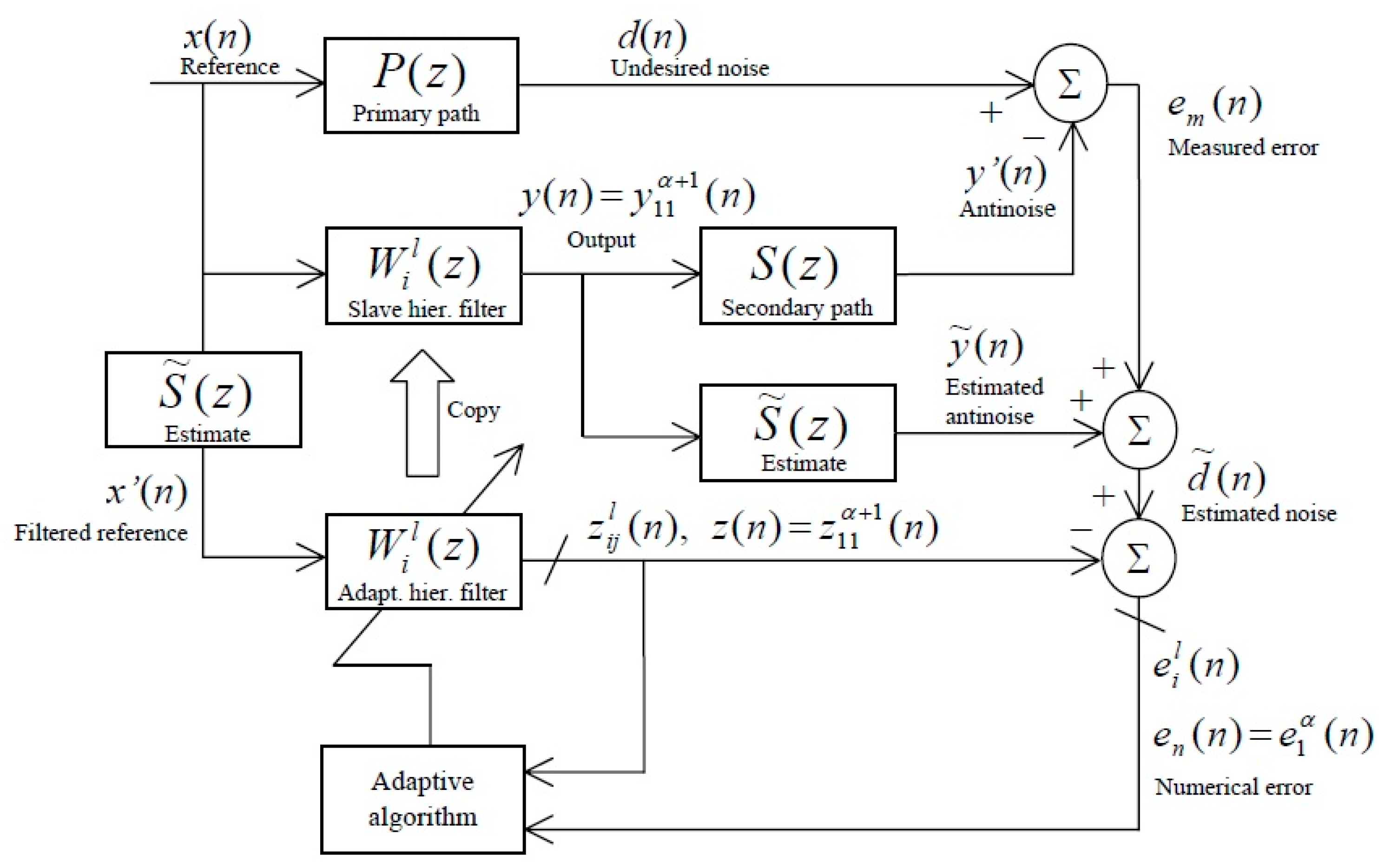
In this section, we propose the Gμ-Mod Fx H Seq LMS algorithm by combining the Mod FxLMS, the HLMS, and the sequential PU LMS with gain in step-size. Our goal is to derive an ANC adaptive algorithm with a faster convergence rate than the conventional FxLMS with a similar computational complexity. Figure 2 shows the block diagram of the proposed algorithm.
According to Figure 2, the filtered reference x ( n ) is the input of the control adaptive filter whereas the reference signal x ( n ) is filtered by a slave filter, which is a copy of the control adaptive filter. By cascading the slave filter and the estimate of the secondary path S ˜ ( z ) , and then by passing the reference signal x ( n ) through the resulting filter, one can obtain an estimation y ˜ ( n ) of the antinoise and hence an estimation d ˜ ( n ) of the undesired noise. Inaccuracy of the secondary path estimate and its effects are discussed in [12,13,14] in the context of filtered x LMS algorithms. At that stage, the output z ( n ) of the adaptive control filter is directly subtracted from the estimated noise d ˜ ( n ) to provide the numerical error e n ( n ) .
One may find in [30] a complete review of techniques of estimation of the error signal using signal processing algorithms. As this error is used to update the adaptive control filter, the limitations imposed on the step-size μ for the standard version of the FxLMS algorithm are now overcome. Let us now focus our attention on the hierarchical filter. Given the number L of taps at the first level of the hierarchy, the number of subfilters at the lth level is given by
N l = L r = 1 l β r = r = 1 α β r r = 1 l β r = r = 1 + 1 α β r
where βl denotes (with this notation, we implicitly assume that the subfilters at the same level have the same number of taps and this number may vary from one level to another) the number of weights of a subfilter at level l, varying from 1 to α. As the subfilter length may vary from one level to another, the step-size bound of every subfilter can be different. In the sequel, the coefficients of the ith hierarchically arranged subfilter impulse response at the lth level are denoted as
w i l ( n ) = [ w i 1 l ( n )   w i 2 l ( n )     w i β l l ( n ) ] , 1 l α ,   1 i   N l
where w i j l denotes the weight for the jth tap of the ith subfilter at the lth level. In addition, z i j l and y i j l , respectively, denote the input signals of the the jth tap of the ith subfilter at the lth level of the adaptive and the slave hierarchical filters. The outputs of the adaptive and the slave hierarchical filters, respectively denoted as z ( n ) and y ( n ) , are given by the last loop of the multilevel filtering, that is, z ( n ) = z 11 α + 1 ( n ) and y ( n ) = y 11 α + 1 ( n ) . The error signal of the ith subfilter at the lth level is denoted as e i l . These error signals are obtained by subtracting the output of every subfilter from the estimated noise d ˜ ( n ) . It should be noted that the necessity of using the estimated noise d ˜ ( n ) to update the subfilters placed at the intermediate levels of the hierarchy is already solved as we use the Mod FxLMS version of the ANC algorithm. Figure 3 shows the architecture of a 2-level hierarchical filter. In this example, the number of subfilters at levels 1 and 2 are N 1 = L / β and N 2 = 1 , respectively. The number of coefficients of every subfilter at levels 1 and 2 are β and L/β, respectively.
The main drawback of the HLMS is the high computational complexity inherently associated to its multi-level structure.
Sequential PU of the coefficients of the hierarchical filter are used to reduce the computational complexity. PU are applied to every coefficient at every level, of the hierarchical organization of taps, from the first tap of the first subfilter to the last tap of the last subfilter. For instance, in Figure 3, the shadowed coefficients of the hierarchical filter are the N-equally-spaced taps that have to be updated at a given time n. At the following iterations of the updating process, namely n + 1, n + 2, …, n + N − 1, the next subsets of equally spaced coefficients of the hierarchical filter are updated.
Due to PU, the algorithm suffers from a reduction in convergence rate as N increases. Then, by using the gain in step-size, the slower convergence rate of the sequential PU adaptive algorithm can be compensated. The strategy hence gives the same performance as that of the full updates algorithm in terms of convergence rate, but with lower computational complexity. In previous works [29], this strategy is analyzed in the context of a conventional adaptive FIR filter.
The Gμ—Mod Fx H Seq LMS deals with periodic disturbances. These periodic noises, such as engine noise, are very often the subject of cancellation in ANC applications. This is due to two reasons. First, these disturbances are the most annoying and, second, it is usually easy to find a good reference signal to cancel them. In the Algorithm 1, the Gμ—Mod Fx H Seq LMS algorithm is given:
Algorithm 1 Gμ—Mod Fx H Seq LMS algorithm
for i = 1 to # iterations/* MAIN LOOP*/
   y i   j 1 ( n ) = x ( n ) /*First level of slave hierarchical filter is filled with x ( n ) */
/* SLAVE HIERARCHICAL FILTER */
  for l = 1 to α/* From first to top (α) level of the hierarchy fo*/
     for i = 1 to r   =   l + 1 α β r /* From first to last subfilter at each level */
      /* Computing the output of every subfilter */
       y p   q l + 1 ( n ) = w i   l T ( n )   y i   l | p = i β l ,   q = i i 1 β l β l
     end of for (i)
  end of for (l) → y ( n ) = y 1   1 α + 1 ( n ) /* END OF SLAVE HIERARCHICAL FILTER */
   y ˜ ( n ) = s ˜ T ( n )   y 11 α + 1 ( n ) /* Computing the antinoise signal where */
/* s ˜ ( n ) = [ s ˜ 1 s ˜ 2 s ˜ L ] T and */
/* y 1   1 α + 1 ( n ) = [ y 11 α + 1 ( n ) y 1   1 α + 1 ( n L s + 1 ) ) ] T */
/* Measured error e m ( n ) = d ( n ) y ( n ) */
   d ˜ ( n ) = y ˜ ( n ) + e m ( n )   /* Computing the estimated noise */
   x ( n ) = s ˜ T ( n )   x ( n ) /* Filtering the reference x ( n ) = [ x ( n ) x ( n L s + 1 ) ) ] T */
   z i   j 1 ( n ) = x ( n ) /* First level of adaptive hierarchical filter is filled with x ( n )
*//* ADAPTIVE HIERARCHICAL FILTER */
  for l = 1 to α/* From first to top level of the hierarchy */
      for i = 1 to r   =   l + 1 α β r /* From first to last subfilter at each level */
      /* Computing the output of every subfilter */
       z p   q l + 1 ( n ) = w i   l T ( n )   z i   l | p = i β l ,   q = i i 1 β l β l
       e i l ( n ) = d ˜ ( n ) w i   l T ( n )   z i   l ( n ) /* Computing the error of every subfilter */
     for j = 1 to β l /* For every tap, Sequential partial updates */
         if ( k ( ( i 1 ) β l + j ) + 1 )   mod   N = = 0
          w i   j l ( k + 1 ) = w i   j l ( k ) + G μ   μ l   e i l ( n )   z i   j l ( n )
         else
          w i   j l ( k + 1 ) = w i   j l ( k )
         end of if
     end of for (j)
    end of for (i)
  end of for (l) → z ( n ) = z 1   1 α + 1 ( n ) /* END OF ADAPTIVE HIERARCHICAL FILTER */
end of for (n)/* END OF MAIN LOOP */

3. Convergence Analysis

In the first part of this section, we establish the assumptions taken into account in the convergence analysis. In the second sub-section, we derive the gain in step-size of the Gμ—Mod Fx H Seq LMS algorithm.

3.1. Assumptions in the Convergence Analysis

In [29], we have derived an upper bound on the step-size for the Fx sequential PU LMS algorithm updating a conventional FIR filter. This analysis is based on two assumptions, namely the independence theory between the reference signal and the filter weights, and the slow convergence condition (The reader is referred to [29] for more information on the assumption of independence theory and the slow convergence condition. Despite the fact that such assumptions might be initially questionable when dealing with periodic inputs, we confirm in [29] the feasibility of assuming both conditions in the analysis of a FIR-based Fx sequential PU LMS strategy to attenuate periodic disturbances).
When using a more complex filtering structure [25] based on hierarchically arranged subfilters w i l ( n ) , 1 l α ,   1 i N , the overall convergence of the hierarchical structure is assumed to be constrained by the hierarchical arranged subfilter w s l o w ( n ) that converges with the slowest convergence rate. By applying to w s l o w ( n ) the convergence analysis for a conventional FIR filter recalled in the Appendix A, one can obtain the analytical expression of the gain in step size of the Gμ—Mod Fx H Seq LMS algorithm.
Let us now give the criteria to recognize the slowest subfilter w s l o w ( n ) of the arrangement. The convergence conditions of w i l ( n ) , 1 l α ,   1 i N , depends on its length and on its input signal. The larger the subfilter is, the smaller the maximum step-size is. Therefore, the larger the subfilter is, the slower the convergence will be (See Appendix A.3 of the Appendix A, where the dependence of the step-size bound on the length of a filter is derived). As far as the input signal is concerned, Woo [25] states that the influence of the input on the convergence is related to the level of the subfilter in the hierarchy. The eigenvalue spread of the input-signal autocorrelation matrix becomes smaller from level l to level l + 1 because the hierarchical structure tends to average the eigenvalues of the related input-signal autocorrelation matrix. Then, assuming that the number of taps β of every subfilter is the same, regardless the position in the hierarchy, the bottle-neck in the convergence process is located at the subfilters of the first level.
Nevertheless, in our approach, every hierarchically arranged subfilter, and more particularly w s l o w ( n ) , is updated by the sequential PU algorithm. Therefore, we have to consider that the logical subfilter (we consider a logical subfilter as the set of N-equally-spaced taps of a filter updated at every iteration of the updating process according to a sequential LMS algorithm with decimation factor N (see Appendix A)) is formed by the subset of β/N coefficients of the β-length subfilter w s l o w ( n ) . These β/N coefficients are updated in one iteration of the sequential LMS algorithm with decimation factor N. Therefore, the convergence condition of the hierarchical arrangement is established on the basis of the joint convergence of the N logical subfilters into which the slowest subfilter w s l o w ( n ) is decomposed. Having determined the element that limits the convergence rate, we derive the gain in step-size for the hierarchical structure in the next section.

3.2. Gain in Step-Size of the Gμ—Mod Fx H Seq LMS Algorithm

Results derived in the Appendix A for a conventional FIR filter (theoretical derivation of the gain in step-size for a conventional adaptive FIR filter whose coefficients are partially updated according to the sequential LMS algorithm can be found in the Appendix A.4 of the Appendix), are extended to the β-length slowest subfilter of the hierarchy w s l o w ( n ) , when sequential PU with decimation factor N are applied to the hierarchical filter. The role of this slowest subfilter can be played by any of the subfilters located at the first level of the hierarchy.
To obtain more easily the factor by which the step-size parameter µ of the proposed algorithm can be increased with regard to the step-size of the full updates approach, we impose the use of the same value for µ for every subfilter of the hierarchy. Then, we consider the bound on the step-size of the hierarchical filter as the maximum value of µ that ensures convergence in all the subfilters.
Since β is shorter than the total number L of taps at the first level of the hierarchy ( β = L α typically), and, provided that the decimation factor N > 1, the number β/N of subfilter coefficients that are effectively updated per iteration is small. When β/N is not integer, this ratio must be rounded to the nearest integer either towards zero, β / N , or towards infinity, β / N . In that case, the β-length hierarchical subfilter is decomposed into β N β / N logical subfilters of length β / N , and N β + N β / N logical subfilters of length β / N . The β / N -length logical subfilters have a slower convergence rate than that of the β / N -length logical subfilters (in Appendix A.3 of the Appendix A, it is proved that the larger an adaptive filter, the smaller the bound on its step-size). As there is at least one β / N -length logical subfilter per iteration at the first level, the convergence rate of a β / N -length logical subfilter determines the convergence of the hierarchy of the subfilters.
For the sake of simplicity to obtain the dependence of the gain in step-size on the length β and on the decimation factor N, let a single tone of normalized frequency f0 be the input signal of the hierarchical structure. Thus, the gain in step-size is given by
G μ ( 1 , f 0 , β ,   N )   = max { 1 4 [ β   ±   sin ( β 2 π f 0 ) sin ( 2 π f 0 ) ] } max { 1 4 [ β N   ±   sin ( β N 2 π N f 0 ) sin ( 2 π N f 0 ) ] } .
We have carried out several computer-based simulations to compare the theoretical prediction given by Equation (4), with the experimental results. This study confirms that this worst-case hypothesis makes it possible to accurately predict the behavior of the experimental convergence process. In Section 4.1, we provide a comparison between the theoretical gain in step-size, given by Equation (4), with the affordable increase in step-size obtained by MATLAB simulation.

4. Simulation Results

The purpose of this section is twofold. First, we compare the theoretical prediction of the gain in step-size—Equation (4)—with computer-based results. Then, we analyze the relevance of the Gμ—Mod Fx H Seq LMS algorithm in an ANC system when dealing with harmonic disturbances.

4.1. Gain in Step-Size: Simulation vs. Theory

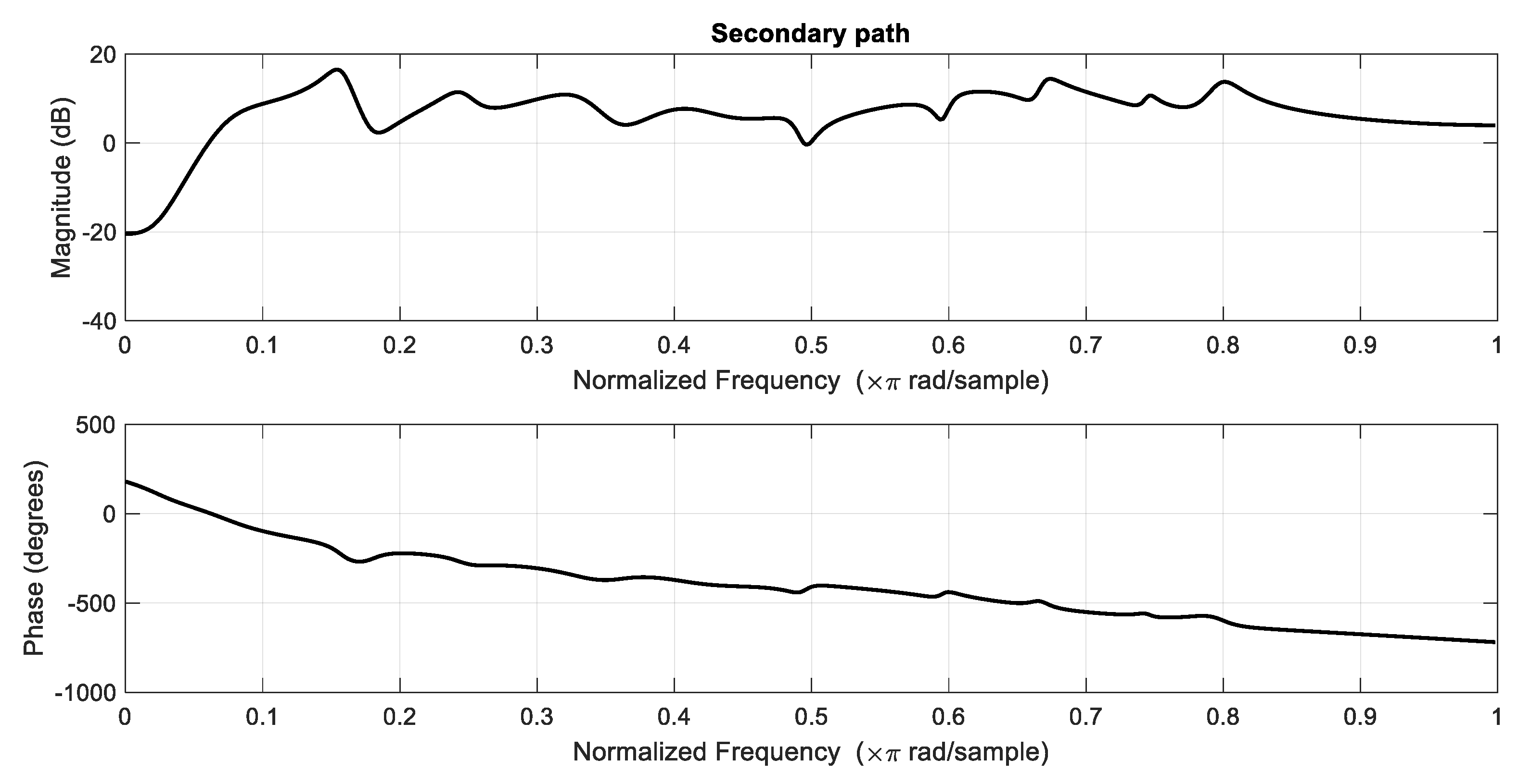
Let us consider the following simulation protocol: it corresponds to the 1 × 1 × 1 arrangement, that is, 1 reference sensor, 1 error microphone and 1 secondary source (see Figure 1). The first level of the hierarchical filter consists of 384 coefficients organized in 16 subfilters of 24 taps. Therefore, in the second level of the hierarchy, one has a 16-length subfilter. The reference is a single sinusoidal signal whose frequency varies in 41.6 Hz steps from 41.6 to 4000 Hz. The sampling frequency is 8000 samples/s. Primary and secondary paths are set to filters modelling real-world active noise control systems. We use filters 25th order IIR filters provided by Kuo and Morgan in [6] (in the book-attached floppy disc featuring C and assembly programs for implementing ANC systems). Plant models from this well-known reference are considered among researchers in the topic as a valid benchmark. Figure 4 and Figure 5 show the magnitude and phase of the primary and secondary paths, respectively.
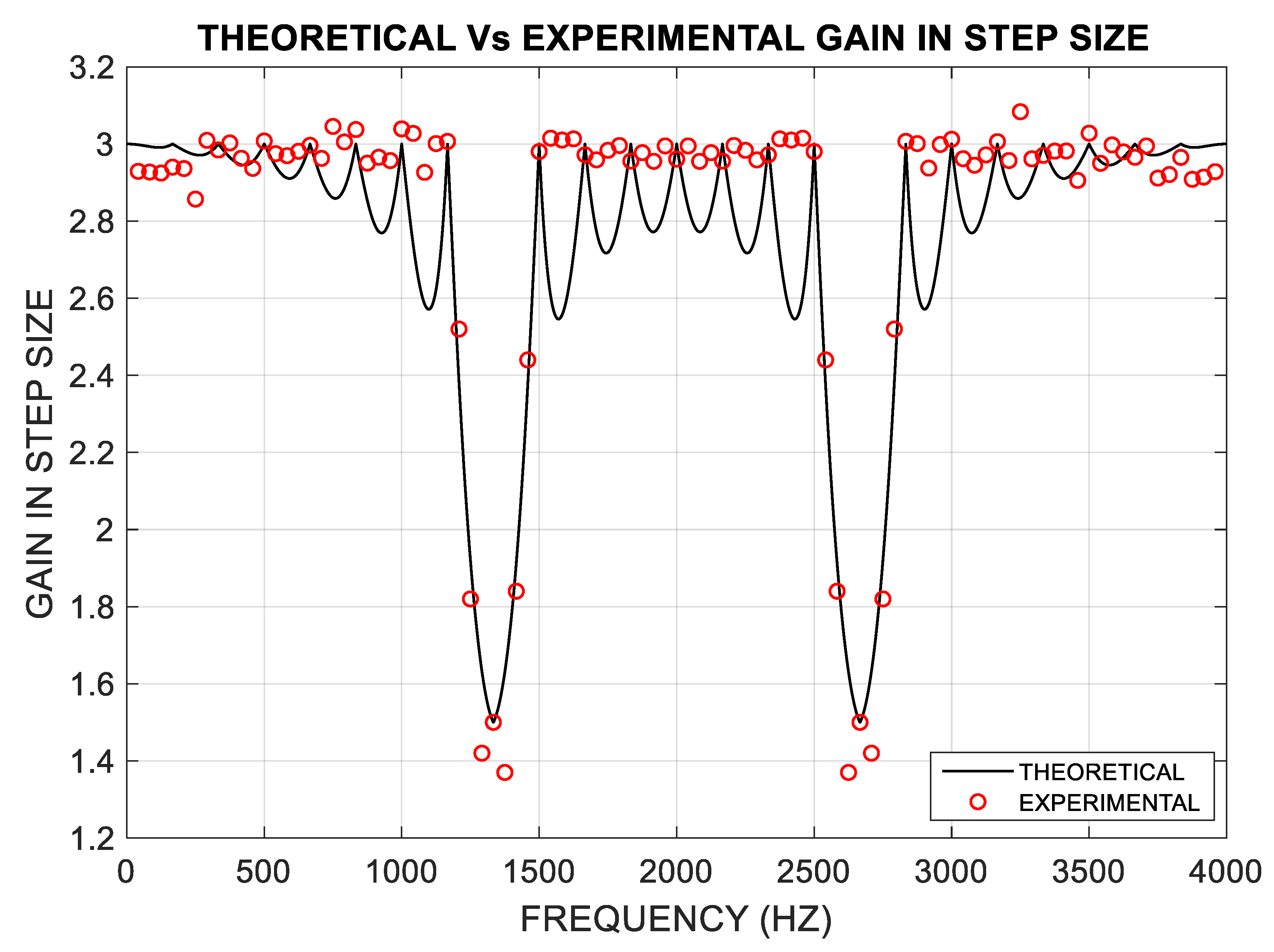
The output of the primary path is then disturbed by additive zero-mean white Gaussian noise η ( n ) , with a signal-to-noise ratio SNR of 27 dB. The decimation factor N of the PU strategy is set to 3. To obtain a previous coarse estimate of the experimental upper bound μ ˜ m a x , the step-size is increased until divergence appears. At that stage, one focuses more carefully on the neighborhood of that value by making the step-size varying with an increment equal to 10 3 μ ˜ m a x . The comparison between the simulated and the experimental results is shown in Figure 6.
According to Figure 6, the predicted gain in step-size is in good agreement with the experimental results obtained by simulations. It should be noted that in both cases, the gain in step-size corresponds to the decimation factor N, namely 3, for most of the frequencies apart from the notches that appear at 1333.3 Hz and 2666.6 Hz. Moreover, the experiment confirms that the global convergence of the hierarchical controller is determined by the convergence of the 24-length subfilter at the first level.

4.2. Comparative Study between Different ANC Algorithms

In this part, we compare the Gμ—Mod Fx H Seq LMS algorithm with three approaches:
(a)
Standard FxLMS, with a L-length FIR adaptive filter [4];
(b)
Mod FxLMS with a L-length FIR adaptive filter [12,13];
(c)
Mod H FxLMS with L coefficients at the first level of the hierarchical filter.
The computational complexity and the convergence rate are the two criteria we take into account. As in the previous sub-section, the 1 × 1 × 1 arrangement is chosen for the ANC system. Nevertheless, in this second example, the selected reference signal x ( n ) is a multi-tone signal defined as follows
x ( n ) = cos ( 2 π 90 F s n ) + 5 cos ( 2 π 100 F s n ) + 3   cos ( 2 π 110 F s n ) + 2   cos ( 2 π 300 F s n ) +   3 cos ( 2 π 320 F s n ) + cos ( 2 π 340 F s n ) + 2 cos ( 2 π 650 F s n ) + 5 cos ( 2 π 665 F s n ) + 4   cos ( 2 π 680 F s n )
where the sampling frequency FS is set to 1600 samples/s. With such an input, the conventional FxLMS algorithm shows difficulties to rapidly cancel the undesired noise. Primary and secondary paths are the 25th order IIR filters shown in Figure 4 and Figure 5, respectively. The output of the primary path is disturbed by an additive zero-mean white Gaussian noise η ( n ) leading to a SNR = 50 dB. The off-line estimate of the secondary path is carried out by an adaptive FIR filter of 128 coefficients.
To obtain a feasible DSP-board implementation, L is set to 625 taps. When the hierarchy is used, these taps are organized in 25 subfilters of β = 25 weights. Therefore, at the second level, there is one subfilter of β = 25 taps.
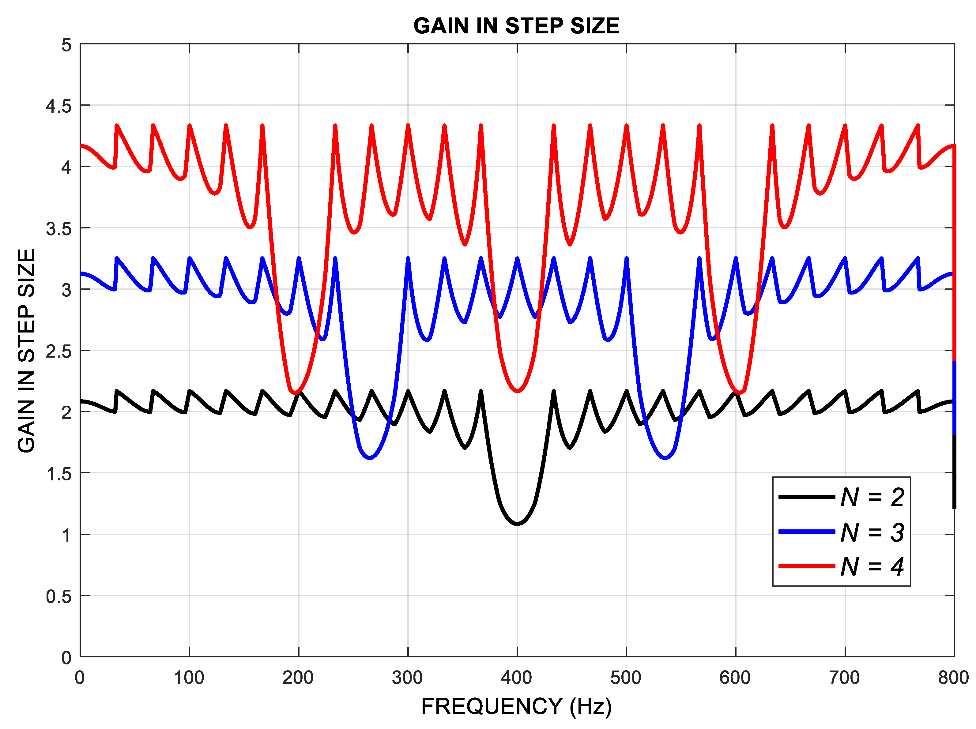
The performance of the proposed algorithm is tested for different values of the decimation factor N, namely N = 2, 3, and 4. Figure 7 shows the theoretically predicted gain in step-size, defined by Equation (4), over the frequency band of interest for N = 2, 3, and 4.
The frequency response of the gain in step-size depends on the decimation factor and exhibits N 1 notches, located at { i F s / 2 N } i = 1 , , N 1 . Therefore, the PSD of the undesired disturbance has to be taken into account to select the decimation factor. Figure 8a,b compares the learning curves of the FxLMS algorithm, the Modified FxLMS algorithm and the Gµ—Mod Fx H Seq LMS, for N = = 1 and 4, respectively. The learning curves are averaged over 500 realizations. To carry out a fair comparison of algorithms, we have adjusted the step sizes to make the FxLMS and the Modified FxLMS converge to the same residual noise level that the proposed algorithm reaches.
Given Figure 8, it can be affirmed that the Modified FxLMS algorithm (blue) converges faster than the standard FxLMS (black), and when a hierarchical filter is included (red), the convergence rate is further boosted. Although the hierarchical filter accelerates the convergence rate of the modified FxLMS (this was the reason to include a hierarchical structure), it presents an inherent drawback: including the hierarchical filter implies an increase in the computational complexity. To minimize this negative effect, we included partial updates of the coefficients with a decimation factor N. In so doing, the convergence rate is reduced proportionally to N, unless gain in step size is applied.
By increasing the step size in a factor Gµ = N, the convergence rate and the residual error of our approach are approximately the same when N is modified. As the reference signal given by Equation (5) does not include harmonics in the vicinity of the notches presented in the gain in step size when N = 4 (see Figure 7), full gain in step-size can be applied, and performance of the Gµ -Mod Fx H Seq LMS algorithm in both cases—(a) full updates, N = Gµ = 1 and (b) partial updates N = Gµ = 4—are similar in terms of convergence rate and residual error, with a significant reduction in the computational cost when partial updates are implemented.
As far as the computational complexity is concerned, let us assume for the sake of simplicity that the length of every subfilter is β, regardless of its position in the hierarchy. Therefore L = βα. In addition, we recall that Ls is the length of the off-line estimate of the secondary path.
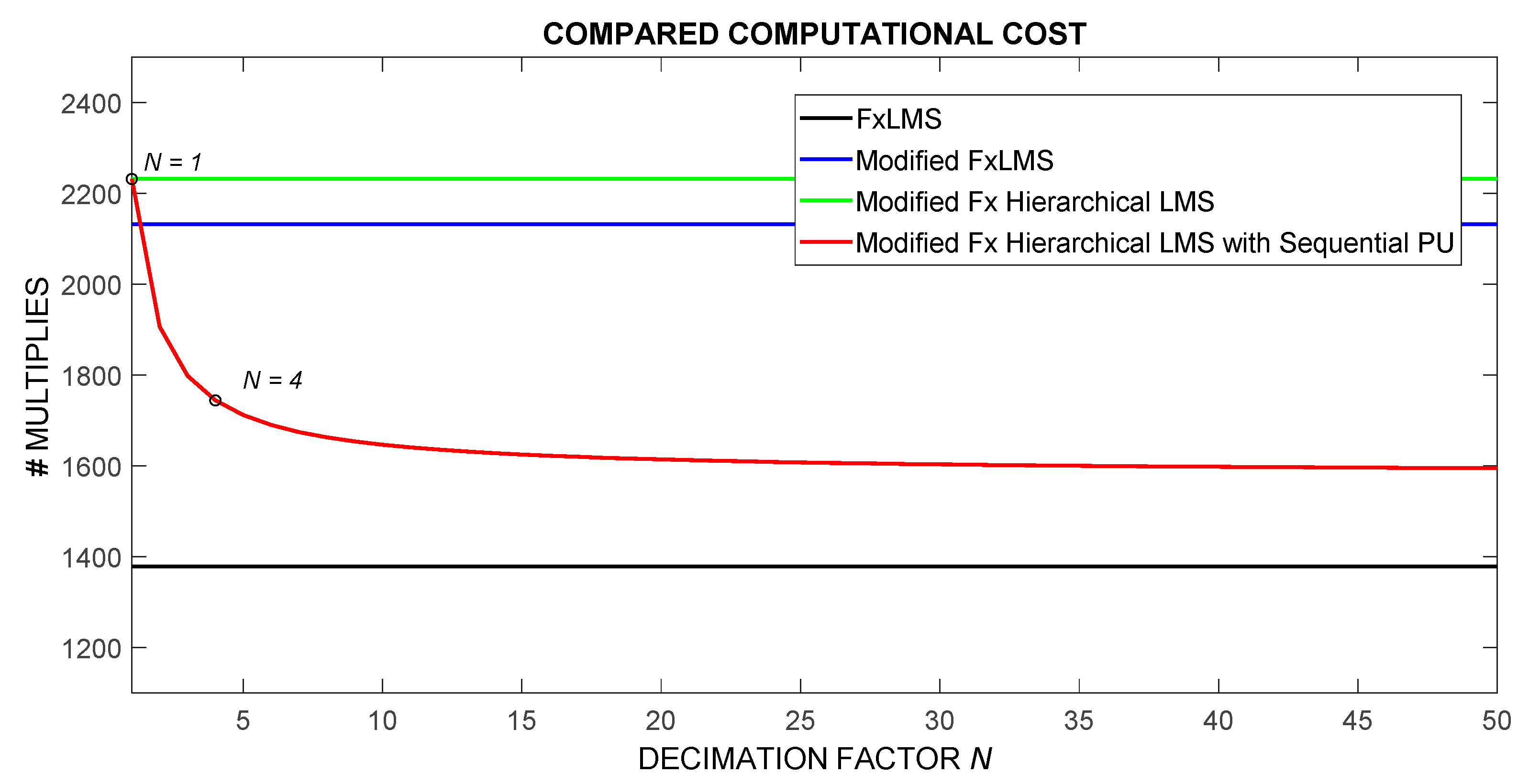
According to Table 1, the modified version of the FxLMS requires L + Ls extra multiplications with regard to the computational complexity of the conventional FxLMS algorithm. When the hierarchical filter is used, the computational complexity is further increased because of the multi-level arrangement. Finally, our algorithm has the advantage of reducing the computational complexity thanks to the PU strategy. Figure 9 compares the computational complexities of different ANC algorithms when the decimation factor N varies from 1 to 50.
Only the sequential PU algorithm depends on the decimation factor N. The L = 625 taps are organized in 25 subfilters of β = 25 weights. The computational complexity for the decimation factors N = 1 and N = 4 are marked with a circle over the curve. According to Figure 9, it is not necessary to use a very large decimation factor to reduce the computational complexity of the proposed algorithm to the order of that of the conventional FxLMS. If the decimation factor N is set to 4, the computational complexity of the modified Fx hierarchical LMS algorithm with sequential PU shows an evident reduction with regards to the full updates (N = 1) algorithm. In our example, setting the decimation factor N = 4 leads to a good compromise between computational complexity and convergence rate. In addition, it is well suited with the disturbance PSD. More generally, we suggest the practitioner to take into account these above features to select the parameters of our approach.

5. Conclusions

This work presents a contribution to the selection of the step-size used in the modified Fx hierarchical LMS adaptive algorithm with sequential PU. The periodic-input signal case is studied, and it is verified that, under certain conditions, the stability range of the step-size is increased compared to the full updates modified Fx hierarchical LMS.
The algorithm we propose is based on the sequential PU of the coefficients of a hierarchical filter and on the controlled increase in the step-size of the adaptive algorithm.
To boost up the convergence rate of the approach, we suggest combining the modified FxLMS and the hierarchical LMS algorithm. Nevertheless, in so doing, the increase in the computational complexity turns out to be the main drawback. Therefore, to reduce the number of operations required per cycle, we propose to use the sequential PU algorithm. Finally, the existence of an affordable increase in step-size—or gain in step-size—allows the global control strategy to compensate for the lack of adaptation of most of the coefficients, even when the number of operations per iteration is significantly reduced due to PU.
The proposed algorithm has the advantage of increasing the convergence rate of the well-known FxLMS algorithm, with a moderate increase in the computational complexity. The proposed method can be used in ANC systems to attenuate periodic disturbances, if the harmonics of the disturbance are not located at frequencies where the gain in step-size exhibits notches. The width and exact location of these notches depend on the system parameters.

Author Contributions

Conceptualization, P.R.L. and G.P.-N.; methodology, P.R.L. and G.P.-N.; software, P.R.L., R.M.F. and F.A.M.; validation, P.R.L. and G.P.-N.; formal analysis, P.R.L., R.M.F.; investigation, P.R.L., R.M.F.; resources, P.R.L., R.M.F. and F.A.M.; data curation, P.R.L., R.M.F. and F.A.M.; writing—original draft preparation, P.R.L.; writing—review and editing, P.R.L. and G.P.-N.; visualization, R.M.F. and F.A.M.; supervision, P.R.L. and G.P.-N.; project administration, P.R.L. and G.P.-N.; funding acquisition, P.R.L. and G.P.-N. All authors have read and agreed to the published version of the manuscript.

Funding

This research was funded by “Cátedra Devoture de Tecnología para el Ser Humano. Universidad de Zaragoza”.

Institutional Review Board Statement

Not applicable.

Informed Consent Statement

Not applicable.

Data Availability Statement

The data presented in this study are available on request from the corresponding author.

Conflicts of Interest

The authors declare no conflict of interest.

Appendix A

The purpose of this Appendix A is to derive analytical expressions of the step-size bound and the gain in step-size (i.e., the factor by which the step-size parameter of an adaptive filter driven by a sequential PU algorithm can be increased to compensate for its intrinsic lower convergence rate due to PU) when the sequential PU LMS algorithm is used to update the coefficients of an adaptive FIR filter. The study is based on the eigenvalues of the autocorrelation matrix of the periodic filter input. To help the reader, we recall results that have been already presented in, namely, Equations (A7) and (A8), Equations (A14)–(A17), and Equations (A24) and (A25), because they allow us to determine in this paper:
(a) The dependence of the step-size bound of the adaptive algorithms on the length of the adaptive filter. The analysis includes not only the conventional full updates LMS algorithm, but also the sequential PU LMS algorithm with decimation factor N,
(b) The gain in step-size of the sequential PU LMS algorithm.
The traditional LMS algorithm analysis can be extended to the FxLMS algorithm, widely used in the field of ANC systems, under certain assumptions, namely the independence between the input signal and the filter weights, the slow convergence condition, and the exact off-line estimate of the secondary path [20], as long as the input signal corresponds to the reference signal filtered by the estimate of the secondary path. Thus, in the sequel we focus our attention on the LMS algorithm.
The Appendix A is organized in four sub-sections. Firstly, one recalls the expression of the autocorrelation matrix of the input vector. Then, the analytical expression of the eigenvalues of a harmonic input signal is presented in Appendix A.2. It makes possible to express the step-size bound and the gain in step-size in and Appendix A.3 and Appendix A.4, respectively.

Appendix A.1. Autocorrelation Matrix of the Decimated Input Vector of the Sequential PU LMS Algorithm

Let be the L-length LMS-filter vector response updated as follows
w ( n + 1 )   =   w ( n )   +   μ   e ( n )   x ( n )
where µ is the step-size of the adaptive algorithm, e(n) the error signal between the output of the filter and the desired response, and x ( n ) = [ x ( n )   x ( n 1 )     x ( n L + 1 ) ) ] T the L × 1 input vector of the LMS algorithm, whose Toeplitz autocorrelation matrix is given by
R   =   E [ x ( n ) x T ( n ) ] .
when the sequential PU LMS algorithm is used with decimation factor (N < L; in addition, and for the sake of simplicity, we assume throughout the paper that the ratio L/N is integer) N, the weights of the L-length filter are updated by means of the following recursion
w ( n + 1 )   =   w ( n )   +   μ   e ( n )   I 1 + n mod N ( N ) x ( n )
where the L × L matrix I p ( N ) , with p = 1 + n   m o d   N N   is defined by
I p ( N ) = d i a g (   0 0 p 1 1 0 0 N 1 1 0 0 N 1 1 0   0 1 0 0 N p   )
As one has
  I p ( N ) x ( n ) = [ 0 0 p 1 x ( n p + 1 ) 0 0 N 1 x ( n p N + 1 ) 0 0 x ( n L + N p + 1 ) 0 0 N p ] T
Equation (A3) leads to
w p + α N ( n + 1 ) = { w p + α N ( n ) + μ   e ( n )   x ( n p α   N + 1 ) f o r   α = 0 , , L N 1 w p + α N ( n ) o t h e r w i s e .
At that stage, let us introduce the pth L/N-length “logical subfilter”, with p cyclically varying from 1 to N. It is defined by the set of L/N equally-spaced taps [ w p   w p + N   w p + 2 N     w p + L N ] of the L-length filter response vector w ( n ) . At time n + p 1 , where p = 1 + n   m o d   N , the pth logical subfilter is updated by means of Equation (A6). Therefore, the N subfilters require the same signal input samples to be updated. They are stored in the vector x ( N ) ( n ) that corresponds to the N-decimated version of x ( n ) .
x ( N ) ( n ) = [ x ( n )   x ( n N )   x ( n 2 N )     x ( n L + N ) ] T .
At time n + N , x ( N ) ( n ) is shifted, inserting a new sample at the position formerly given by the index n, while the older data is lost. See Table A1, which shows the subsets of coefficients of the filter response vector w ( n ) = [ w 1   w 2     w L ] T to be updated according to Equation (A3) during N + 1 consecutive iterations and their corresponding samples of the input vector.
Table A1. Coefficients to be updated—defining a logical subfilter—during N + 1 consecutive iterations and their corresponding samples of the input vector.
# IterationCoefficients That Form the Logical Subfilter Updated at the Current IterationSamples of the Input Vector Used to Update the Logical Subfilter
1 [ w 1   w 1 + N   w 1 + 2 N     w L N + 1 ] T [ x ( n )   x ( n N )   x ( n 2 N )     x ( n L + 1 ) ) ] T
N [ w N   w 2 N   w 3 N     w L ] T [ x ( n )   x ( n N )   x ( n 2 N )     x ( n L + 1 ) ) ] T
N + 1 [ w 1   w 1 + N   w 1 + 2 N     w L N + 1 ] T [ x ( n + N )   x ( n )   x ( n N )     x ( n L + N + 1 ) ) ] T
In light of Equation (A7), the (L/N) × (L/N) Toeplitz autocorrelation matrix   R ( N ) of the decimated input vector x ( N ) ( n ) is given by
R ( N ) =   E [ x ( N ) ( n ) x ( N ) T ( n ) ] .
In the sequel, the convergence properties of the (L/N)-length logical subfilters is analyzed based on the eigenvalues of the autocorrelation matrix R ( N ) .

Appendix A.2. Eigenvalues of the Autocorrelation Matrix of a Periodic Signal Consisting of K Harmonics

Let us assume that the input signal x ( n ) of an adaptive filter is defined as follows
x ( n )   =   k   =   1 K C k cos ( 2 π k f 0 n   +   φ k )  
where f 0 is the normalized fundamental frequency, { ϕ k } k = 1 , , K the initial random phases mutually independent and uniformly distributed from 0 to 2π and { C k } k = 1 , , K the amplitudes of the harmonics. Given Equation (A9), the autocorrelation function of input signal x ( n ) can be expressed as
r x x ( τ )   =   k   =   1 K C k 2 2 cos ( 2 π k f 0 τ )   .
Therefore, the autocorrelation matrix of the input vector x ( n ) can be expressed as the sum of K matrices R k of size L × L as follows
R   = k = 1 K C k 2   R k
where
R k   =   1 2 { 1 cos ( 2 π k f 0 ) cos [ 2 π k ( L 1 ) f ] cos ( 2 π k f 0 ) 1 cos ( 2 π k f 0 ) cos [ 2 π k ( L 1 ) f ] cos ( 2 π k f 0 ) 1 }   .
The largest eigenvalue λ k , m a x ( k f 0 ) of each matrix R k is given by [31]
λ k , max ( k f 0 )   =   max { 1 4 [ L   ±   sin ( L 2 π k f 0 ) sin ( 2 π k f 0 ) ] }  
where the subscript k refers to the index of the submatrix R k .
According to the triangle inequality [32], appendix E, the largest eigenvalue of a sum of matrices is bounded by the sum of the largest eigenvalues of each of its components. Therefore, the largest eigenvalue λ t o t , m a x of R is bounded by
λ tot , max     k   =   1 K C k 2 λ k , max ( k f 0 )   =   k   =   1 K C k 2 max { 1 4 [ L   ±   sin ( L 2 π k f 0 ) sin ( 2 π k f 0 ) ] }  
where the subscript tot refers to the whole autocorrelation matrix R .
As far as the sequential PU LMS algorithm with decimation factor N is concerned, the convergence condition of the whole filter might be translated to the parallel convergence of N logical subfilters of length L/N updated by a N-decimated input signal x ( N ) ( n ) [29]. Adjusting the above approach to the case of sequential PU LMS, where the size of the autocorrelation matrix is L/N and the sampling frequency is divided by N, we deal with K matrices R k ( N ) of size (L/N) × (L/N) defined by
R k ( N )   =   1 2 { 1 cos ( 2 π N k f 0 ) cos [ 2 π N k ( L N 1 ) f ] cos ( 2 π N k f 0 ) 1 cos ( 2 π N k f 0 ) cos [ 2 π N k ( L N 1 ) f ] cos ( 2 π N k f 0 ) 1 }   .
Therefore, the largest eigenvalue λ k , m a x   ( N ) ( k f 0 ) of each matrix R k ( N ) can be expressed as follows
λ k , max ( N ) ( k f 0 )   =   max { 1 4 [ L N   ±   sin ( L N 2 π k N f 0 ) sin ( 2 π k N f 0 ) ] } .
Considering the triangle inequality, the largest eigenvalue λ t o t , m a x   ( N ) of the (L/N) × (L/N) matrix R ( N )   = k = 1 K C k 2   R k ( N ) is bounded by
λ tot , max ( N )     k   =   1 K C k 2 λ k , max ( N ) ( k f 0 )   =   k   =   1 K C k 2 max { 1 4 [ L N   ±   sin ( L N 2 π k N f 0 ) sin ( 2 π k N f 0 ) ] }   .
It should be noticed that for N = 1 the sequential PU LMS algorithm reduces to the conventional full updates LMS algorithm and Equations (A16) and (A17) reduce to Equations (A13) and (A14), respectively.

Appendix A.3. Effect of the Length of the Filter on the Step-Size Bound

In this section, we analyze the effect of the length of an adaptive filter on the maximum value of the step-size that ensures convergence of the adaptive algorithm. The analysis deals with the case of the reference signal defined in Equation (A.9). The dependence of the step-size bound on the number of coefficients of the filter is studied not only for the full updates LMS algorithm, but also for the sequential PU LMS algorithm with decimation factor N.
(a)
Full updates LMS algorithm
Let the input signal of the LMS algorithm be the periodic signal given by Equation (A9). The convergence in mean of the weights of the filter is guaranteed if the step-size satisfies the inequality [33]
0 < μ L M S < 2 λ tot , max .
Thus, combining Equations (A14) and (A18), we obtain a more restrictive bound on the step-size that ensures convergence in mean.
0 < μ L M S < 2 k   =   1 K C k 2 max { 1 4 [ L   ±   sin ( L 2 π k f 0 ) sin ( 2 π k f 0 ) ] } .
Hence, the bound on μ L M S depends on the frequency f 0 , the length of the filter L, and the weights C k of the input signal. To simplify the graphical representation of the bound, the input signal of a L-length adaptive filter updated by the conventional LMS algorithm is defined by the following single tone of normalized frequency f 0 .
x ( n )   =   cos ( 2 π f 0 n   +   φ )   .
Due to Equations (A19) and (A20), the bound on the step-size is then given by
0 < μ L M S < 2 max { 1 4 [ L   ±   sin ( L 2 π f 0 ) sin ( 2 π f 0 ) ] } = 2 λ tot , max .
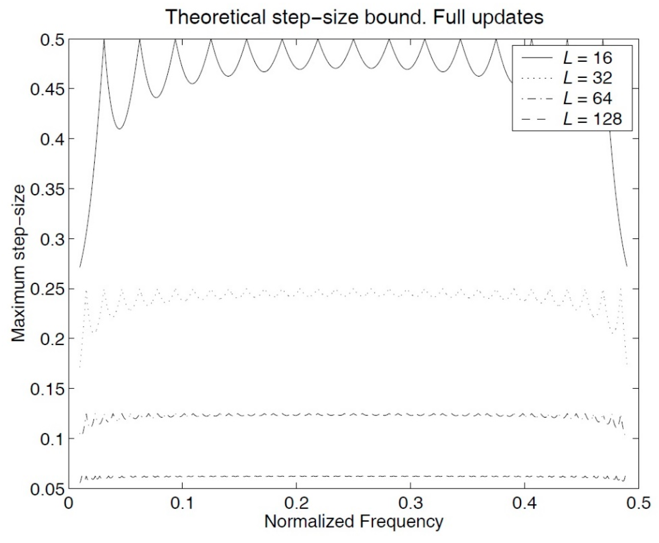
Figure A1 shows the size bound of the conventional LMS algorithm for L = 16, 32, 64, and 128. The normalized frequency of the input vector varies from 0 to 0.5.
Figure A1. Step-size bound of the conventional full updates LMS algorithm for different filter lengths, L = 16, 32, 64, and 128. The input vector is a single tone whose normalized frequency varies from 0 to 0.5.
Applsci 11 00344 g0a1
According to Figure A1, and considering that a large step-size guarantees fast convergence rate, we conclude that a shorter filter can converge faster than a large one.
(b)
Sequential PU LMS algorithm.
Let the L × 1 input vector of the sequential PU LMS algorithm be given by the N-decimated version x ( N ) ( n ) of the periodic signal x ( n ) expressed by Equation (A9). A similar analysis as the one carried out in the previous section for the conventional LMS algorithm yields a more restrictive bound on the step-size that ensures convergence in mean for the case of the sequential PU LMS algorithm.
0 < μ S e q L M S < 2 k   =   1 K C k 2 max { 1 4 [ L N   ±   sin ( L N 2 π k N f 0 ) sin ( 2 π k N f 0 ) ] } < 2 λ tot , max ( N ) .
This bound on μ S e q L M S depends on the frequency f 0 , the length of the filter L, the weights of the input signal C k , and the decimation factor N. As we did in the previous section to simplify the graphical representation of the bound, we reduce the number of harmonics of the input signal to K = 1. In so doing, the L × 1 input vector of the sequential PU LMS algorithm is given by the N-decimated version x ( N ) ( n ) of a sinusoidal signal defined in Equation (A20). The bound on the step-size is then reduced to
0 < μ S e q L M S < 2 max { 1 4 [ L N   ±   sin ( L N 2 π N f 0 ) sin ( 2 π N f 0 ) ] } = 2 λ tot , max ( N ) .
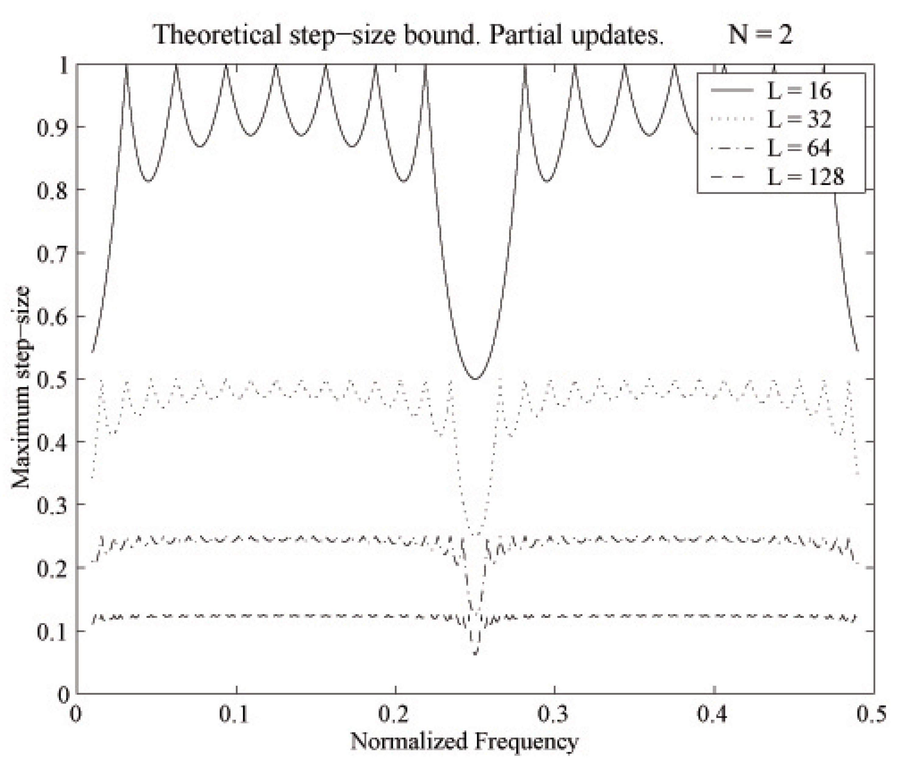
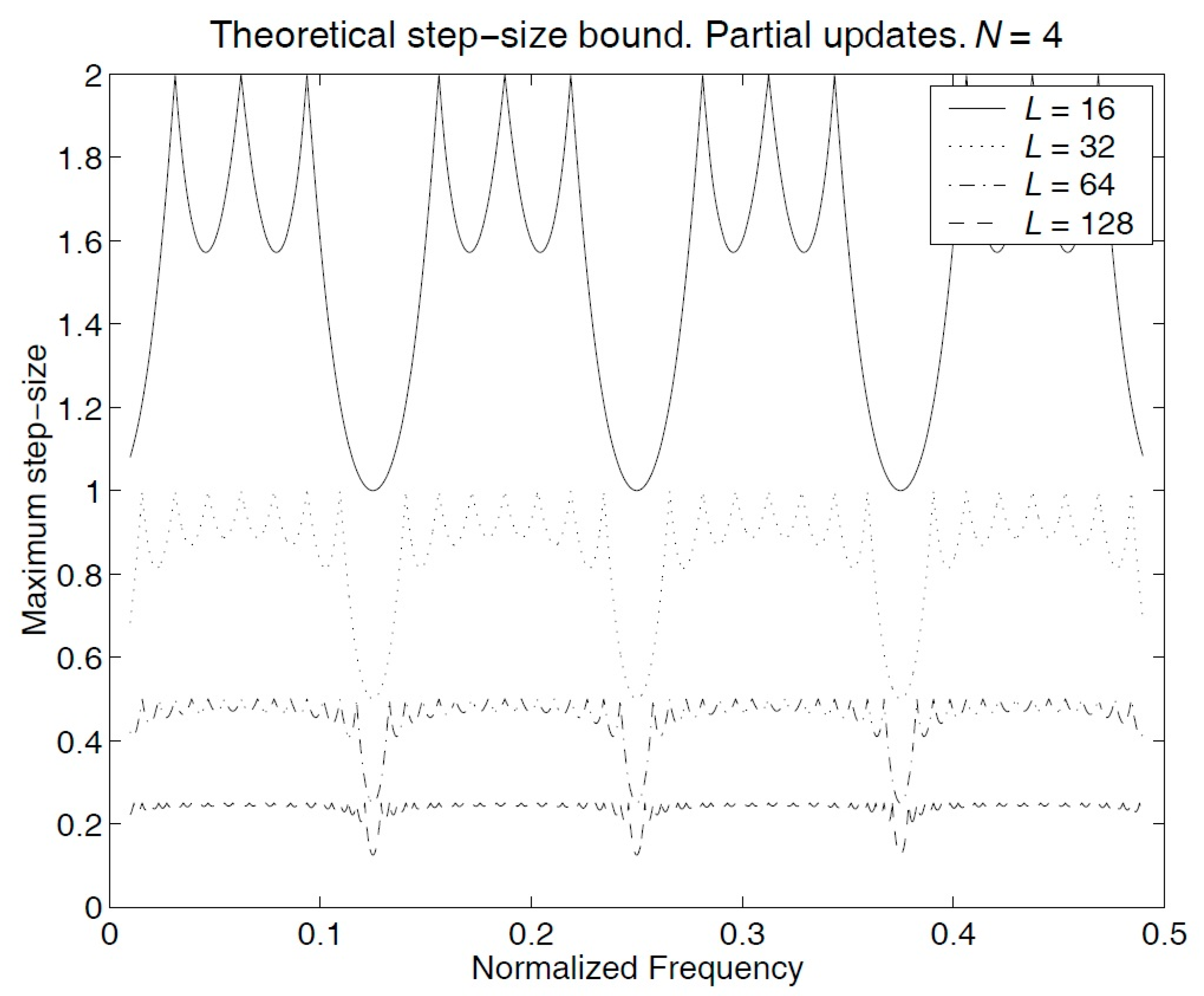
Figure A2 and Figure A3 show the size bound of the sequential PU LMS algorithm given by Equation (A23) for decimation factors N = 2 and N = 4, respectively. Results are given for L = 16, 32, 64, and 128. The normalized frequency of the input vector varies from 0 to 0.5.
Figure A2. Step-size bound of the sequential PU LMS algorithm with decimation factor N = 2 for different filter lengths, L = 16, 32, 64, and 128. The input vector is an N-decimated single tone whose normalized frequency varies from 0 to 0.5.
Applsci 11 00344 g0a2
Figure A3. Step-size bound of the sequential PU LMS algorithm with decimation factor N = 4 for different filter lengths, L = 16, 32, 64, and 128. The input vector is an N-decimated single tone whose normalized frequency varies from 0 to 0.5.
Applsci 11 00344 g0a3
According to Figure A2 and Figure A3, and considering that a large step-size guarantees fast convergence rate, we conclude that a shorter filter can converge faster than a large one when the sequential PU LMS is used.

Appendix A.4. The Gain in Step-Size
By defining the gain in step-size Gµ as the ratio between the bounds on the step-sizes in two different cases—N > 1 (sequential PU LMS) and N = 1 (conventional LMS)—we obtain the factor by which the step-size parameter can be multiplied when the adaptive algorithm uses sequential PU
G μ ( K , f 0 , L , N )   =   b o u n d { μ S e q L M S } b o u n d { μ L M S }   =   2 max { λ tot , max ( N ) } 2 max { λ tot , max }   =   k   =   1 K C k 2 λ k , max ( k f 0 ) k   =   1 K C k 2 λ k , max ( N )   ( k f 0 ) =   k   =   1 K C k 2 max { 1 4 [ L   ±   sin ( L 2 π k f 0 ) sin ( 2 π k f 0 ) ] } k   =   1 K C k 2 max { 1 4 [ L N   ±   sin ( L N 2 π k N f 0 ) sin ( 2 π k N f 0 ) ] } .
To more easily visualize the dependence of the gain in step-size on the length of the filter L and on the decimation factor N, the number of harmonics of the input signal is set to K = 1. Now, the gain in step-size, that is, the ratio between the bounds on the step-size when N > 1 and N = 1, is given by
G μ ( 1 , f 0 ,   L ,   N )   =   b o u n d { μ S e q L M S } b o u n d { μ L M S }   =   max { 1 4 [ L   ±   sin ( L 2 π f 0 ) sin ( 2 π f 0 ) ] } max { 1 4 [ L N   ±   sin ( L N 2 π N f 0 ) sin ( 2 π N f 0 ) ] }   .
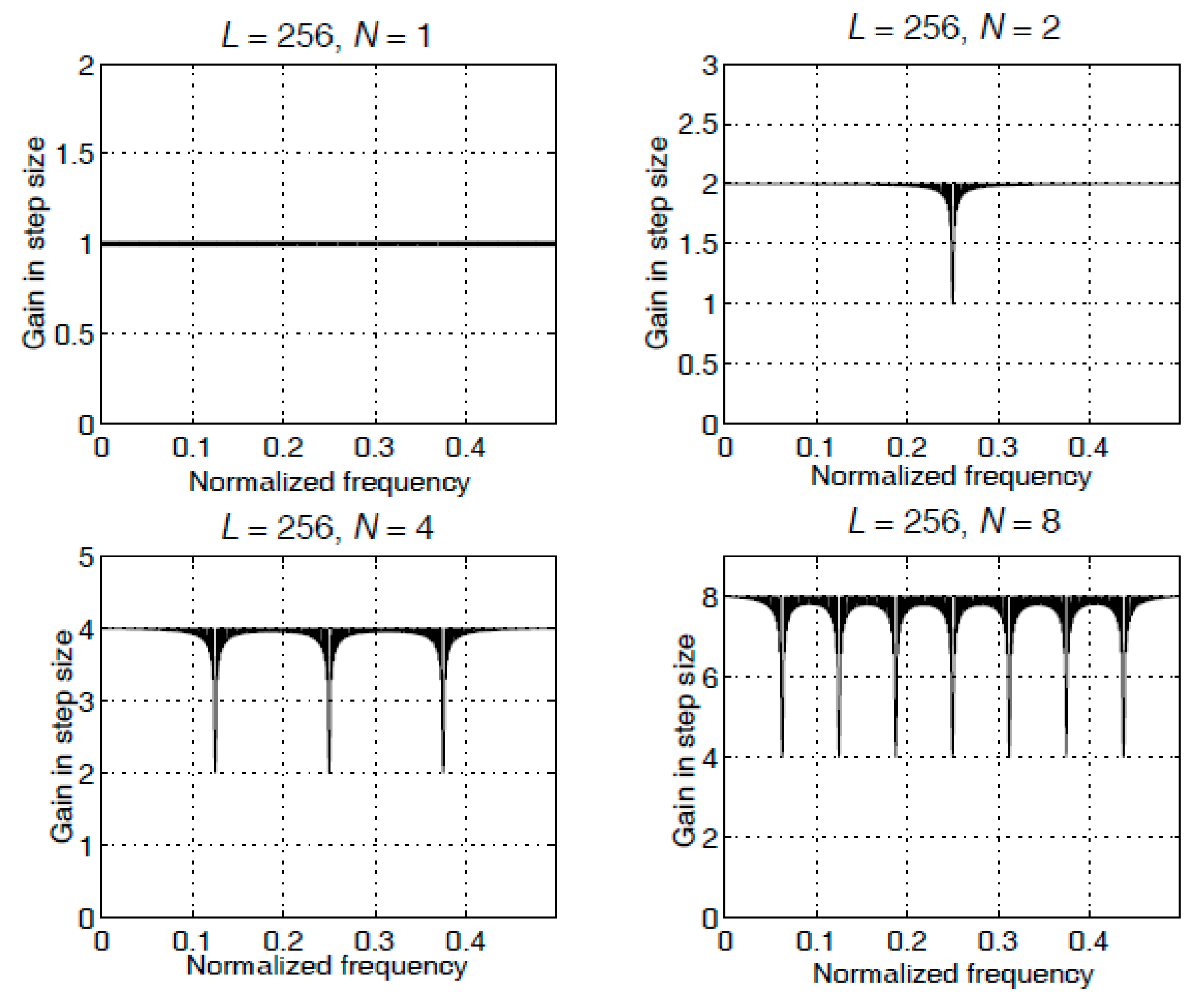
Figure A4 and Figure A5 show, respectively, the gain in step-size for a single tone when different decimation factors and different filter lengths are considered. According to Figure A4 and Figure A5 show that the step-size can be multiplied by N as long as certain frequencies, at which a notch in the gain in step-size appears, are avoided. The location of these critical frequencies, as well as the number and width of the notches, will be analyzed as a function of the sampling frequency F s , the length of the adaptive filter L, and the decimation factor N. According to Equations (A24) and (A25), with increasing decimation factor N, the step-size can be multiplied by N and, as a result of that affordable compensation, the sequential PU LMS algorithm convergence is as fast as the full updates LMS algorithm as long as the undesired disturbance is free of components located at the notches of the gain in step-size.
Figure A4. Gain in step-size for a single tone and different decimation factors, N = 1, 2, 4, and 8. The length of the filter is set to L = 256 taps.
Applsci 11 00344 g0a4
Figure A5. Gain in step-size for a single tone and different filter lengths, L = 8, 32, and 128 with decimation factor N = 2.
Applsci 11 00344 g0a5

References

  1. Stansfeld, S.; Haines, M.; Brown, B. Noise and Health in the Urban Environment. Rev. Environ. Health 2000, 15, 43–82. [Google Scholar] [CrossRef] [PubMed]
  2. Basner, M.; Babisch, W.; Davis, A.; Brink, M.; Clark, C.; Janssen, S.; Stansfeld, S. Auditory and non-auditory effects of noise on health. Lancet 2014, 383, 1325–1332. [Google Scholar] [CrossRef] [Green Version]
  3. Minichilli, F.; Gorini, F.; Ascari, E.; Bianchi, F.; Coi, A.; Fredianelli, L.; Licitra, G.; Manzoli, F.; Mezzasalma, L.; Cori, L. Annoyance Judgment and Measurements of Environmental Noise: A Focus on Italian Secondary Schools. Int. J. Environ. Res. Public Health 2018, 15, 208. [Google Scholar] [CrossRef] [PubMed] [Green Version]
  4. Attenborough, K.; Vér, I.L. Sound-absorbing materials and sound absorbers. In Noise and Vibration Control Engineering; Principles and Applications; John Wiley & Sons, Inc.: New York, NY, USA, 2005. [Google Scholar]
  5. Munjal, M.; Galaitsis, A.G.; Vér, I.L. Passive silencers. In Noise and Vibration Control Engineering: Principles and Applications Noise; John Wiley & Sons, Inc.: Hoboken, NJ, USA, 2006; pp. 279–343. [Google Scholar]
  6. Kuo, S.; Morgan, D. Active Noise Control Systems: Algorithms and DSP Implementations; Wiley: New York, NY, USA, 1996. [Google Scholar]
  7. Samarasinghe, P.N.; Zhang, W.; Abhayapala, T.D. Recent Advances in Active Noise Control Inside Automobile Cabins: Toward quieter cars. IEEE Signal Process. Mag. 2016, 33, 61–73. [Google Scholar] [CrossRef] [Green Version]
  8. Morgan, D. An analysis of multiple correlation cancellation loops with a filter in the auxiliary path. IEEE Trans. Acoust. Speech Signal Process. 1980, 28, 454–467. [Google Scholar] [CrossRef]
  9. Bjarnason, E. Analysis of the filtered-X LMS algorithm. IEEE Trans. Speech Audio Process. 1995, 3, 504–514. [Google Scholar] [CrossRef]
  10. Vicente, L. Novel FxLMS convergence condition with deterministic reference. IEEE Trans. Signal Process. 2006, 54, 3768–3774. [Google Scholar] [CrossRef]
  11. Yang, F.; Guo, J.; Yang, J. Stochastic Analysis of the Filtered-x LMS Algorithm for Active Noise Control. IEEE ACM Trans. Audio Speech Lang. Process. 2020, 28, 2252–2266. [Google Scholar] [CrossRef]
  12. Boucher, C.C. The effects of modeling error on the performance and stability of active noise control systems. In Recent Advances in Active Control of Sound Vibration; CRC Press: Boca Raton, FL, USA, 1991. [Google Scholar]
  13. Snyder, S.D.; Hansen, C.H. The effect of transfer function estimation errors on the filtered-x LMS algorithm. IEEE Trans. Signal Process. 1994, 42, 950–953. [Google Scholar] [CrossRef]
  14. Tobias, O.J.; Seara, R. Leaky-FXLMS algorithm: Stochastic analysis for Gaussian data and secondary path modeling error. IEEE Trans. Speech Audio Process. 2005, 13, 1217–1230. [Google Scholar] [CrossRef]
  15. Kim, H.-S.; Park, Y. Delayed-X LMS algorithm: An efficient ANC algorithm utilizing robustness of cancellation path model. J. Sound Vib. 1998, 212, 875–887. [Google Scholar] [CrossRef]
  16. Chen, G.; Sone, T.; Saito, N.; Abe, M.; Makino, S. The stability and convergence characteristics of the delayed-x LMS algorithm in ANC systems. J. Sound Vib. 1998, 216, 637–648. [Google Scholar] [CrossRef]
  17. Bjarnason, E. Active noise cancellation using a modified form of the filtered-x LMS algorithm. In Proceedings of the EUSIPCO-92, Sixth European Signal Processing Conference, Brussels, Belgium, 24–27 August 1992. [Google Scholar]
  18. Kim, I.-S.; Na, H.-S.; Kim, K.-J.; Park, Y. Constraint filtered-x and filtered-u least-mean-square algorithms for the active control of noise in ducts. J. Acoust. Soc. Am. 1994, 95, 3379–3389. [Google Scholar] [CrossRef]
  19. Lopes, P.A.C.; Piedade, M.S. The behavior of the modified FX-LMS algorithm with secondary path modeling errors. IEEE Signal Process. Lett. 2004, 11, 148–151. [Google Scholar] [CrossRef]
  20. Ramos, P.; Vicente, L.; Torrubia, R.; López, A.; Salinas, A.; Masgrau, E. On the complexity-performance tradeoff of two active noise control systems for vehicles. In Advances for In-Vehicle and Mobile Systems; Springer: Berlin/Heidelberg, Germany, 2007; pp. 85–96. [Google Scholar]
  21. Rupp, M. Saving complexity of modified filtered-X-LMS and delayed update LMS algorithms. IEEE Trans. Circuits Syst. II Analog Digit. Signal Process. 1997, 44, 57–60. [Google Scholar] [CrossRef]
  22. Douglas, S.C. An efficient implementation of the modified filtered-X LMS algorithm. IEEE Signal Process. Lett. 1997, 4, 286–288. [Google Scholar] [CrossRef]
  23. Yang, F.; Cao, Y.; Wu, M.; Albu, F.; Yang, J. Frequency-Domain Filtered-x LMS Algorithms for Active Noise Control: A Review and New Insights. Appl. Sci. 2018, 8, 2313. [Google Scholar] [CrossRef] [Green Version]
  24. Gaiotto, S.; Laudani, A.; Lozito, G.M.; Riganti Fulginei, F. A Computationally Efficient Algorithm for Feedforward Active Noise Control Systems. Electronics 2020, 9, 1504. [Google Scholar] [CrossRef]
  25. Woo, T.-K. Fast hierarchical least mean square algorithm. IEEE Signal Process. Lett. 2001, 8, 289–291. [Google Scholar]
  26. Macleod, M.D. Performance of the hierarchical LMS algorithm. IEEE Signal Process. Lett. 2002, 9, 436–437. [Google Scholar] [CrossRef]
  27. Tan, L.; Wu, M. Data Reduction in Wireless Sensor Networks: A Hierarchical LMS Prediction Approach. IEEE Sens. J. 2016, 16, 1708–1715. [Google Scholar] [CrossRef]
  28. Douglas, S.C. Adaptive filters employing partial updates. IEEE Trans. Circuits Syst. II Analog Digit. Signal Process. 1997, 44, 209–216. [Google Scholar] [CrossRef]
  29. Ramos, P.; Torrubia, R.; López, A.; Salinas, A.; Masgrau, E. Step Size Bound of the Sequential Partial Update LMS Algorithm with Periodic Input Signals. Eurasip J. Audio Speech Music Process. 2007, 2007, 1–15. [Google Scholar] [CrossRef] [Green Version]
  30. Figwer, J.; Michalczyk, M.I. Notes on a New Structure of Active Noise Control Systems. Appl. Sci. 2020, 10, 4705. [Google Scholar] [CrossRef]
  31. Kuo, S.M.; Tahernehadi, M.; Hao, W. Convergence analysis of narrow-band active noise control system. IEEE Trans. Circuits Syst. II Analog Digit. Signal Process. 1999, 46, 220–223. [Google Scholar] [CrossRef]
  32. Haykin, S. Adaptive Filter Theory; Prentice Hall: Upper Saddle River, NJ, USA, 2002. [Google Scholar]
  33. Widrow, B.; Stearns, S.D. Adaptive Signal Processing; Prentice-Hall: Englewood Cliffs, NJ, USA, 1985; ISBN 978-0-13-004029-9. [Google Scholar]
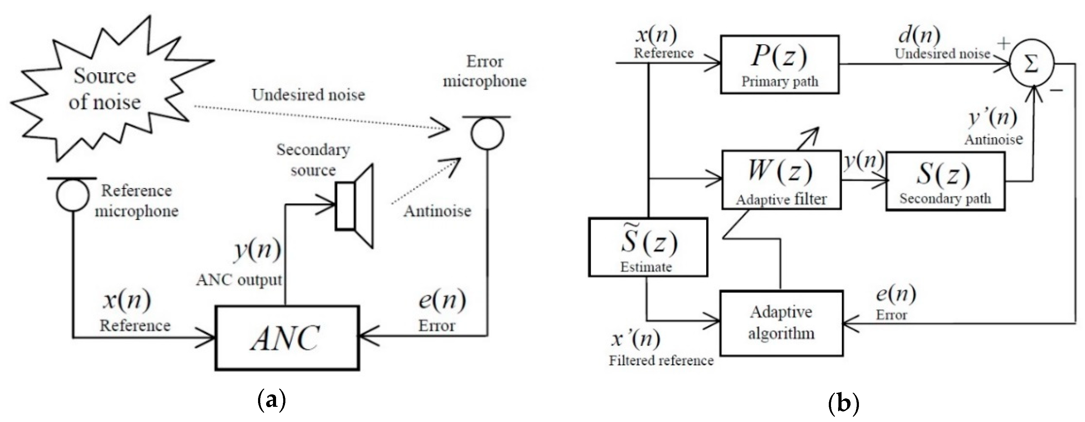
Figure 1. Single-channel active noise control system using the FxLMS algorithm. (a) Physical arrangement of the electro-acoustic elements. (b) Equivalent block diagram.
Applsci 11 00344 g001
Figure 2. Block diagram of the modified filtered-x hierarchical LMS algorithm with sequential partial updates.
Applsci 11 00344 g002
Figure 3. Two-level hierarchical filter.
Applsci 11 00344 g003
Figure 4. Primary path.
Applsci 11 00344 g004
Figure 5. Secondary path.
Applsci 11 00344 g005
Figure 6. Theoretically predicted gain in step-size vs. simulation results of the Gμ—Mod Fx H Seq LMS algorithm in a modelled ANC system.
Applsci 11 00344 g006
Figure 7. Theoretically predicted step-size gain of the Gµ—Mod Fx H Seq PU LMS over the frequency band of interest—from 0 to 800 Hz—for N = 2, 3, and 4. L = 625 taps are organized in 25 subfilters of β = 25 weights.
Applsci 11 00344 g007
Figure 8. Compared performance of FxLMS algorithm, Mod FxLMS algorithm and Gµ—Mod Fx H Seq LMS, (a) N = Gµ = 1 and (b) N = Gµ = 4.
Applsci 11 00344 g008
Figure 9. Computational complexities of different ANC algorithms in terms of the average number of multiplications per iteration.
Applsci 11 00344 g009
Table 1. Comparison of computational complexities of active noise control (ANC) algorithms, in terms of the average number of multiplications per task and iteration, in a single channel implementation of an ANC system.
Task\AlgorithmFxLMSMod FxLMSMod Fx H LMSGµ-Mod Fx H Seq LMS
Computing output of the slave filter- L l = 1 α L β l   β l = 1 α L β l   β
Filtering reference with S ˜ ( z ) L s L s L s L s
Filtering output of the slave filter with S ˜ ( z ) - L s L s L s
Computing output of the adaptive filter L L l = 1 α L β l   β l = 1 α L β l   β
Updates of the coefficients L + 1 L + 1 l = 1 α L β l   ( β + 1 ) l = 1 α L β l   ( β N + 1 )
# Total Mutiplications 2 L + L s + 1 3 L + 2 L s + 1 [ l = 1 α L β l   ( 3 β + 1 ) ] + 2 L s [ l = 1 α L β l   ( 2 β + β N + 1 ) ] + 2 L s
Publisher’s Note: MDPI stays neutral with regard to jurisdictional claims in published maps and institutional affiliations.