Strategies for Extracting Damage Induced AE Signals from Different Type Noise-Like Backgrounds for Carbon-Fibre Reinforced Polymers

Abstract

This paper presents an algorithm for isolating a useful acoustic signal (corresponding to damage accumulation) against the background of a signal used to model the performance of an industrial rotary equipment. Acoustic emission signals induced by deformation and fracture were studied using a uniaxial tensile test on woven laminate samples cut along the fiber and weft directions. The background signal is a random composition of acoustic pulses used to model the performance of an industrial rotary equipment. A comparison of useful and noise signals enables us to develop two algorithms based on frequency filtering of a signal and its decomposition into empirical modes. These algorithms can be used to isolate useful AE pulses against the background of all signal intensities under consideration.

1. Introduction

The steadily increasing requirement for the specific weight of samples designed for automotive, aircraft and space engineering is one of the main reasons to replace metal parts with various composites (carbon–carbon, carbon fiber and fiberglass, woven, knitted, stitched, etc.) [1,2,3,4,5,6]. However, the extensive application of composite parts for critical nodes subjected to constant loads requires continuous monitoring of their performance and fracture (without ceasing the operation of the structure during the repairs).

The most common non-destructive testing method used to solve such problems is an acoustic emission method [7,8,9,10,11,12]. This method records the elastic waves generated by local defects as they appear and grow in a loaded material. Analysis of acoustic emission data provides information on the activity, location and, in some cases, the type of an acoustic emission source [7,10,11,12,13].

Monitoring of structures by AE inevitably raises the question of how the useful signal can be separated from the interference of different nature. The sources of background noise (continuous or discrete) are as follows: the friction of the moving parts of the structure, the passage of technical liquids and gases through pipelines and channels, the flow of incoming air or liquid flow around critical nodes, electromagnetic interference, etc. Approaches to isolating a useful discrete acoustic emission (AE) signal (arising due to material fracture) against continuous or discrete noises can be divided into three types: spatial selection, parametric selection, and filtering.

Spatial selection requires localization of acoustic emission sources with an acceptable error, which in the case of composite materials has proven to be a rather complex problem [14,15,16,17]. Parametric selection is effective when the maximum amplitude of the acoustic emission pulses is, on average, at least 5 dB higher than the amplitude of the noise component. In the opposite case, the problem of original signal filtering has to be solved either to increase the signal-to-noise ratio or to separate the useful signal from the noise-like time-localized signals.

The most common filtering methods are the windowed Fourier transform and discrete wavelet filtering. An important advantage of the wavelet transform is filtration of acoustic emission signals by the hard or soft threshold function (in terms of the given noise model) [18,19,20]. Although the efficiency of the wavelet transform has been already proved, it has some disadvantages. The main disadvantage is the dependence of filtering data and AE characteristics on the basic wavelet [21].

Alternative techniques for analyzing and filtering non-stationary signals are the empirical mode decomposition method and the Prony filtering method [22,23,24,25,26,27]. Empirical mode decomposition method decomposes the signals (via an iterative procedure) into the sum of oscillating signals (empirical modes) selected in accordance with two specified requirements [23,24,25,26,27]. Unlike the wavelet transform, the basis functions are extracted directly from the examined signal with account of its local features. It is known that in some cases the time-frequency resolution of this method is better than the resolution achieved by use of the wavelet transform. Signal filtering is performed in the same way as in the wavelet transform; a certain threshold function is applied to the expansion coefficients in both cases [23,24].

The Prony filtering method decomposes signal into a linear combination of exponential-cosine waves when finding a solution to the problem of residual function minimization. In order to effectively realize signal filtering, it is essential to find optimal decomposition parameters. For this purpose, the available information extracted from a wide range of different sources has been analyzed, which makes it possible to exclude the noisy part of the signal from consideration [22]. In ref. [27], the Prony method was successfully used in the AE analysis for defect detection in rolling bearings. According to [22], this method can be applied for problems associated with seismological and hydrocarbon deposits because it increases the resolution of short seismic signals and identifies zones with anomalous seismic energy scattering (dispersion). The disadvantage of this method is the strong dependence of the decomposition process on chosen parameters.

A fundamentally different approach suggests filtering the noise content in the recorded initial AE signal (the signal remains unconverted). The Kalman filter-based methods are the effective signal processing techniques, which are widely used in radio navigation, guidance and trajectory tracking applications [28,29]. In the framework of the Kalman theory, a wide variety of recursive data processing algorithms have been developed to restore the state of an a priori given dynamic system based on noisy and incomplete measurements. Therefore, the physical features of AE signal propagation are taken into account. In regards to the AE source location, these algorithms require less computational resources and show better accuracy compared to the wavelet transform [28,29].

This approach also includes another research direction that has recently become increasingly popular. It implies the use of artificial neural networks and the concept of deep learning for signal filtering. In [30], a supervised learning neural network was used to develop an algorithm for recovering the AE signal with a signal-to-noise ratio less than one. At the same time, auto-associators (unsupervised learning) have found wide application in speech and image processing technologies [31,32,33,34]. It is known that these algorithms are able to provide more accurate estimates of the signal-to-noise ratios compared to standard filtering methods [32,33,34]. The advantage of these auto-associators is noise separation with maintaining true signal features determined by a training set. Hence, it can be concluded that, this signal processing principle takes into account characteristics of the process under study as Kalman filtration technique.

Choice of a specific method for increasing the signal-to-noise ratio depends in each case on the character of the recorded signal and on the spatio-temporal patterns of its development.

This paper pursues two goals. The first is to investigate generation of acoustic emission signals induced by the fracture in carbon fibre reinforced plastic (CFRP) samples. The second is to develop an algorithm for isolating a useful signal (corresponding to fracture) against the background of a signal that is used to model the performance of an industrial rotary equipment. Therefore, we propose two algorithms designed to reduce various types of background noise.

2. Acoustic Emission from Deformation and Fracture of CFRP Samples

In this study, in order to determine the type of useful AE signals induced by fracture in composite materials, we performed a series of laboratory experiments in which the carbon fibre reinforced plastic samples of various types and geometries were subjected to loads.

2.1. Materials and Experimental Setup

Table 1. Tested samples and loading parameters.

Test	Uniaxial Tensile Test
Material	Woven Laminate		Unidirectional CFRP
Grade	VKU–39		VKU–29
Sample Orientation Relativeto Laying	Warp	Weft	Along Fibers
Loading Rate	1 mm/min

displays information about tested samples and loading parameters. The woven laminate samples cut along the fiber and weft directions and the unidirectional CFRP samples were stretched by uniaxial tensile stresses. Samples for uniaxial tensile tests were prepared according to ASTM D3039 (Figure 1).

An eight-channel hardware–software complex Amsy–5 (Vallen, Germany) was used to register acoustic emission. The pulse waveform signals were recorded at a sampling rate of 2.5 MHz. To amplify the AE signal, we used preamplifiers AEP4 having 34 dB gain; the distance between these preamplifiers and acoustic emission transducers did not exceed one meter.

Analog 95–1450 kHz bandpass filters were installed in front of the ADC to filter the low-frequency noises. DECI SE2MEG–P sensors (frequency range 200–2000 kHz} were used to register AE signals induced by the deformation of the woven laminate samples cut along the weft and warp directions and the unidirectional CFRP samples.

Acoustic emission sensors were attached to the sample surface using cyanoacrylate glue. The AE signals were registered in a discrete mode with a discrimination threshold of 40 dB. The value of the discrimination threshold was selected by analyzing the results of some preliminary experiments with a threshold-less mode of AE data acquisition.

All samples were totally destroyed. After the end of each experiment, multivariable filtering of the acoustic emission data was carried out to remove the pulses caused by the electromagnetic interference and low-frequency noise from the testing machine.

2.2. The Results of the Laboratory Quasi-Static Uniaxial Tensile Tests on CFRP Samples

Acoustic emission activity (one minute signal recording) diagrams for three types of the tested CFRP samples are shown in Figure 2.

Analysis of the data from Figure 2 led us to conclude that the samples of all types are characterized by a monotonic increase in the activity of acoustic emission, which reaches 800–900 pulses per second while approaching the fracture.

In each experiment, the maximum amplitude distribution of AE pulses is the power–law distribution (Figure 3) usually observed during the deformation and fracture of brittle structurally inhomogeneous materials.

The distribution slopes for the woven laminate samples cut along the warp and weft directions are the same, while, in the case of unidirectional CFRP, the slope becomes steeper due to a relative decrease in high-amplitude signals.

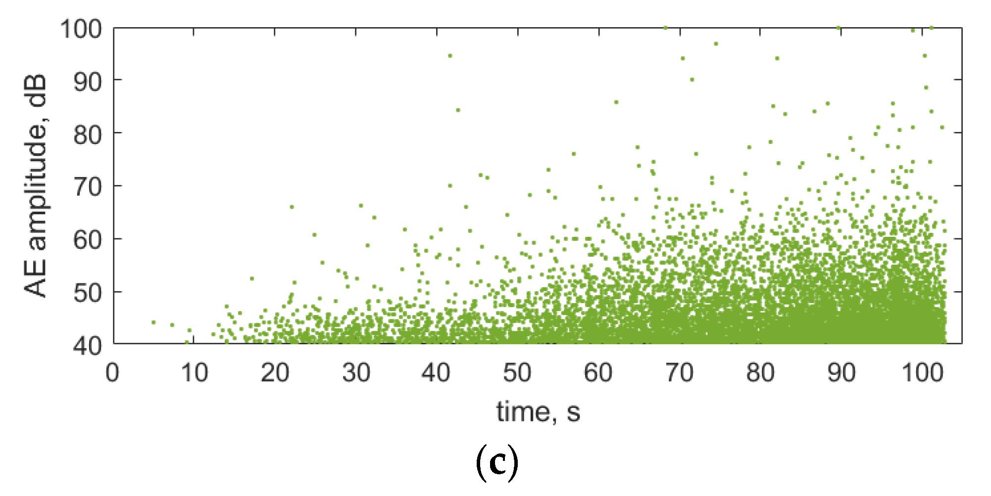
Although the low-amplitude pulses are prevalent in the recorded signals, the medium- and high-amplitude AE pulses can be registered long before fracture, starting from the middle of the first acoustic emission activity stage in each of the three experiments (Figure 4).

Note that in the case of a unidirectional composite material (Figure 4c) this feature is less pronounced, which can be explained by interlayer local delamination.

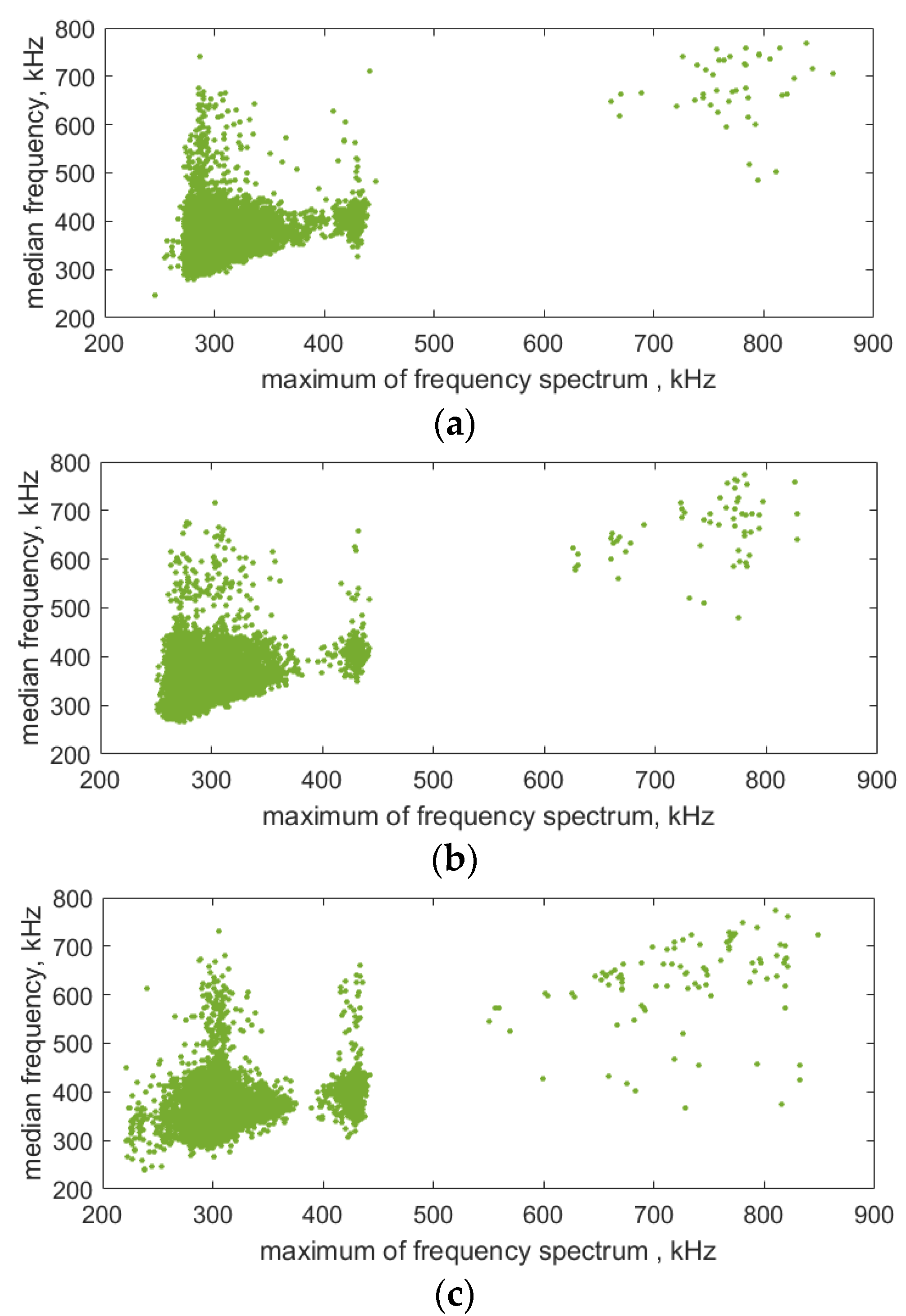
All single pulses can be divided into three groups (with respect to a maximum of frequency spectrum): low-frequency pulses with a maximum of frequency spectrum in the range of 200–350 kHz, medium-frequency pulses with a maximum of frequency spectrum of about 420 kHz, and high-frequency pulses with a maximum of frequency spectrum more than 500 kHz (see Figure 5).

3. Background Noise Modeling

A model signal corresponding to the performance of an abstract rotary equipment is chosen to simulate background noise. We consider two types of acoustic pulses (Figure 6 and Figure 7), recorded during the performance of real industrial rotary equipment. Type 1 pulse (Figure 6) corresponds to a local acoustic event, and Type 2 pulse (Figure 7)—to a continuous noise-like signal.

Let us consider three signals that simulate the performance of the background equipment under different conditions. To do this, we construct background signals by scattering two types of acoustic pulses in a time interval of 0.5 s with a lognormal distribution of the intervals between them (μ–1 ms, σ– 0.5 ms). Figure 8a shows the background signal (the first signal) which corresponds to the single arrival of Type 1 pulses with random intervals. Figure 8b presents the second signal corresponding to the arrival of Type 2 signals with random intervals. A combination of both signals (third signal) is given in Figure 8c.

For further development of the algorithm, the data corresponding to the four levels of intensity (maximum amplitude) has been constructed for each type of the background signal. The maximum signal amplitude ranges from 130 µV (minimum intensity) to 10 mV (maximum intensity).

4. Strategies for Separation of AE Impulses from the Background Signals of Various Types

To develop strategies for isolating AE pulses, we consider the original signal as a composition of different background signals with superimposed AE data recorded in laboratory experiments. We propose two algorithms for separating the useful signal (AE pulses) from the general data stream: frequency filtering and decomposition into empirical modes. The algorithms are used in two typical cases: isolation of a time-localized useful signal from a continuous background signal (Type 3), and isolation of a time-localized useful signal against the background of periodic local acoustic impulses (Type 1).

4.1. Algorithm for Isolating the Useful Signal from the Continuous Noise-Like Background

Local acoustic emission pulses against the background of a continuous signal can be reliably recorded when their maximum amplitude exceeds the maximum background amplitude by at least 5 dB. The ratio of the useful signal maximum amplitude to the background maximum amplitude can be increased by the additional initial data processing. To do this, we assume that the main frequency characteristics of the continuous signal (Type 3 background signal) do not exceed 200 kHz; under laboratory conditions this value is higher. We use the frequency filtering, namely the sixth power Butterworth filter with a cutoff frequency of 200 kHz, to “suppress” the background noise. Figure 9 presents the results of changes in the maximum amplitude of the third background signal of different intensity after partial filtering.

After frequency filtering, the maximum acoustic signal amplitude decreases varying between 13 dB (1 level of signal intensity) and 8 dB (3 level of signal intensity). Therefore, after the frequency filtering with a high-frequency filter, even if the maximum amplitude of the useful signal remains unchanged, the ratio of the useful signal amplitude to the background amplitude increases, by 10 dB on average.

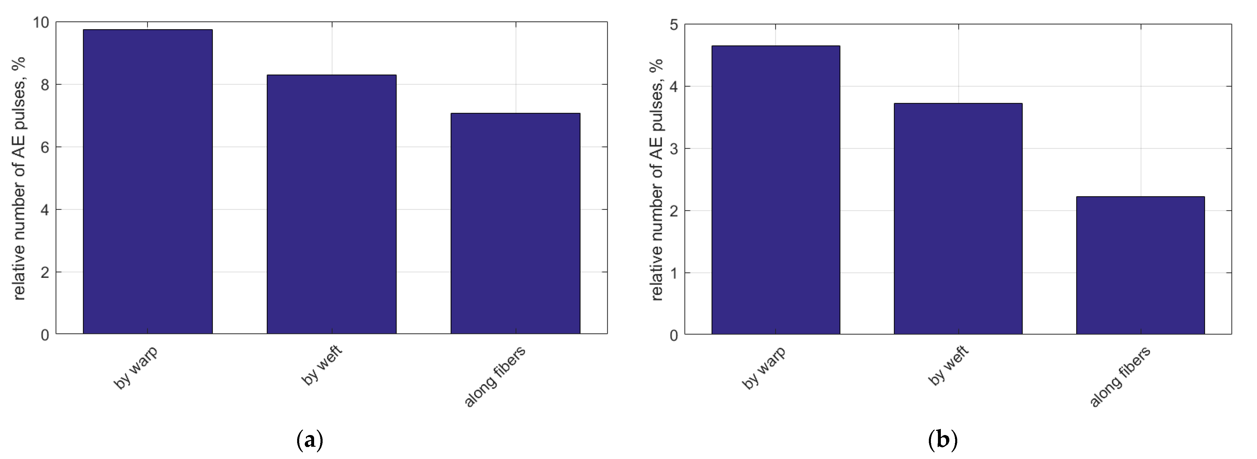
To determine the number of AE pulses that can be reliably recorded at a certain intensity of the background noise, for each type of the laboratory experiments, we have calculated the percentage of AE pulses, the maximum amplitude of which exceeds the maximum amplitude of the Type 3 acoustic signal after frequency filtering by 5 dB. The obtained intensity values are shown in Figure 10.

Analysis of the obtained data has indicated that, at minimum intensity, the background signal level is below the discrimination threshold used for recording AE under laboratory conditions. At increased intensity of the background noise, the situation changes dramatically. A relative number of detected AE pulses decreases, depending on the type of the tested sample, from 2 to 1.15% for the woven laminate sample cut along the warp direction. Regardless of the background noise intensity, the minimum number of detected AE pulses is observed for unidirectional CFRP.

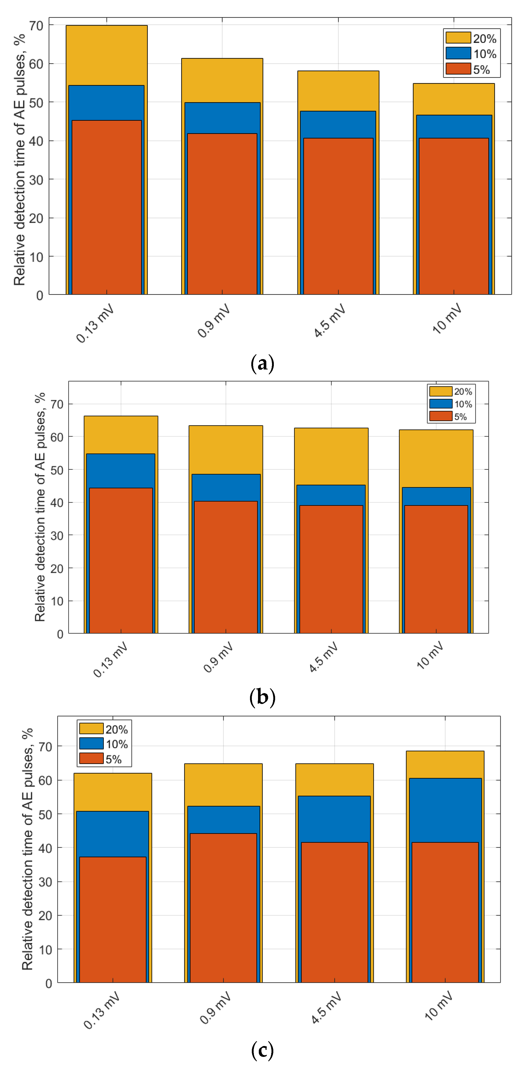
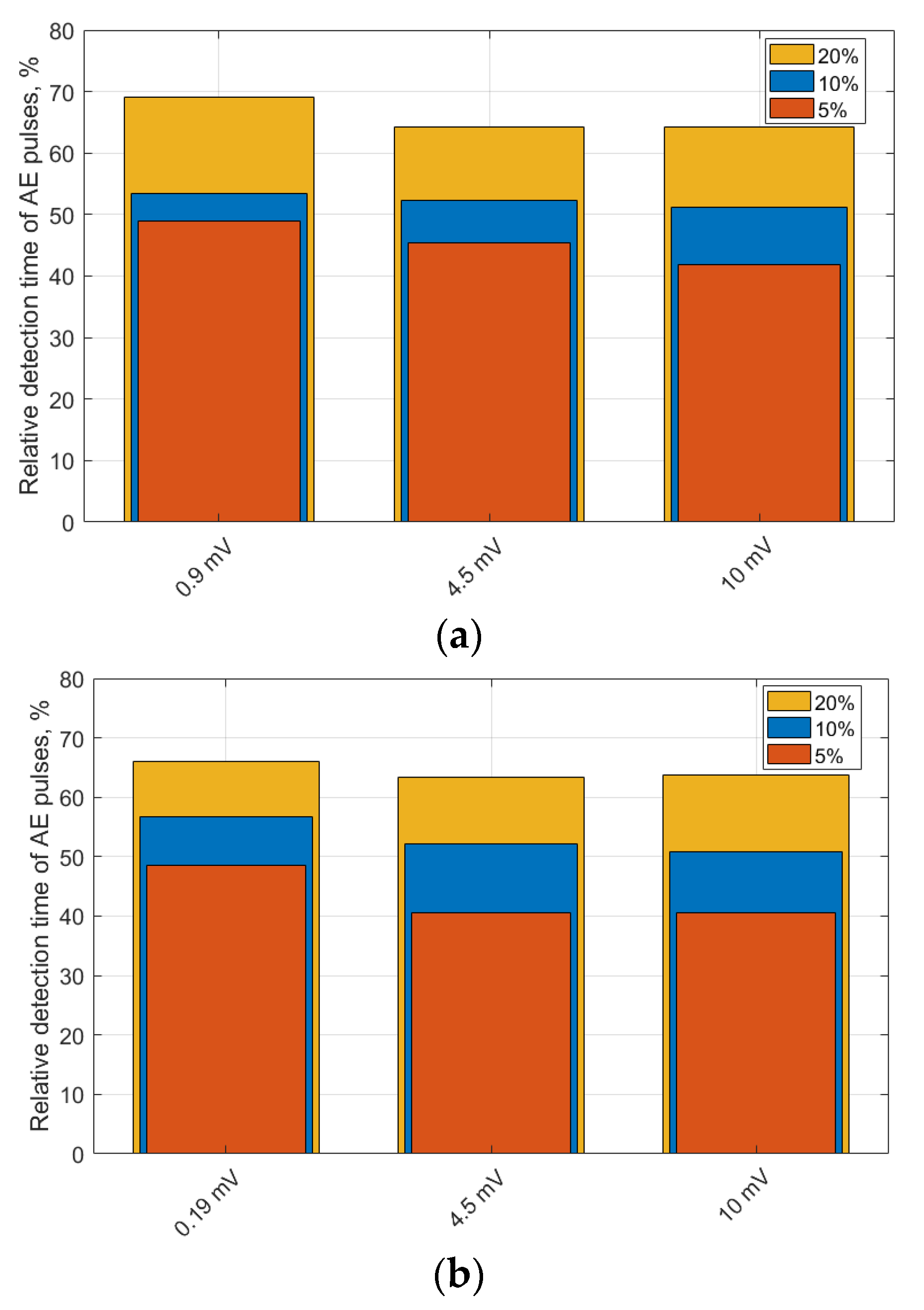
An important indicator of the predictive power of the AE method applied to monitoring real parts is the useful signal detection time versus the time of the “possible” fracture of the part itself. Calculations gave the detection time of the AE pulses comprising 5%, 10% and 20% of the total number of reliably recorded pulses for the sample of a certain type and specified background noise intensity (Figure 11).

On average, for each type of the laboratory experiments, the relative detection time of the AE pulses comprising of 5%, 10%, and 20% of all pulses varies slightly, regardless of the background noise intensity. Five percent of the total volume of AE pulses is recorded in the time interval not exceeding 40% of the sample fracture time, and ten and twenty percent in the interval not exceeding 50% and 60%, respectively.

Despite the fact that the total number of the reliably detected AE pulses for three out of four modes does not exceed a few percent, the time required to register 5, 10, and 20% of these pulses significantly differs from the time of the “possible” fracture of the test object.

The strategy for isolating a useful signal from a continuous noise-like background requires sequential implementation of the following procedures:

• Frequency filtering of the original signal using the high-frequency filter with a cutoff frequency of 200 kHz;
• Isolation of single AE impulses with a maximum amplitude that exceeds the maximum amplitude of the background signal by 5 dB.

4.2. Algorithm for Isolating the Useful Signal against the Background of Periodic Local Acoustic Pulses

In the case of periodic local acoustic pulses of various intensities (Type 1 background signal), the processing strategy depends on the time at which the useful signal appears and on its maximum amplitude. If the acoustic emission pulse occurs in the intervals between the background acoustic pulses (Figure 12), then the processing strategy involves:

• Isolation of a complete set of single pulses;
• Parametric filtering of single pulses, whose spectrum maximum frequency does not exceed 200 kHz, or multiparameter cluster analysis of the entire set of single pulses (the cluster associated with background pulses is excluded from further consideration).

When the useful signal (AE pulse) is superimposed on the background acoustic signal with different degrees of overlapping, the strategy for isolating the useful signal (the ratio of the AE pulse amplitude to the background pulse amplitude increases) depends on the maximum AE pulse amplitude. We use the empirical mode decomposition (EMD) method to increase the ratio of the AE pulse amplitude to the background pulse amplitude. Decomposition of the signal composed of the superimposed AE pulse and the background acoustic pulse (Figure 13) into empirical modes is shown in Figure 14.

As one can see, the high-frequency signal component corresponding to the AE pulse is most fully represented in the first mode, where the value of the second maximum associated with the background pulse is significantly reduced. Thus, to increase the ratio of the AE pulse amplitude to the background pulse amplitude, it is necessary to pass from the initial signal to its first empirical mode. When the difference between the amplitudes of the AE pulse (the amplitude of the AE pulse is less) and the superimposed background pulse is −6.3 dB in the first empirical mode, the local maxima associated with both signal components are equal.

To determine the relative number of reliably detected AE pulses from all the pulses recorded as a detection threshold in laboratory experiments, we take the minimum amplitude of the pulses, the total number of which is more than 1%, minus 6.3 dB. For the maximum intensity of the background signal, the detection threshold was 63.7 dB, for the number 3 intensity was 61.7 dB.

Figure 15 gives the relative number of AE pulses detected in each of the laboratory experiments (uniaxial tension of the woven laminate sample cut along the warp and weft directions and the unidirectional CFRP sample cut along the fiber direction) for different background signal intensities. It is seen that, in the case of periodic local acoustic pulses, the relative number of detected pulses is larger than that in the case of a continuous noise-like signal. Figure 16 presents the relative detection time of the AE pulses comprising of 5, 10, and 20% of all pulses for various background signal intensities.

The results demonstrate that, on average, the detection time for AE impulses comprising of 20% of the total number of impulses does not exceed 70% for all modes and types of the experiments, and the obtained values correlate with the results for the continuous background signal.

Summing up, the strategy for separating a useful signal from the periodic local acoustic pulses with superimposed AE pulses requires sequential implementation of the following procedures:

• Decomposition of the signal into empirical modes and construction of the first of these modes;
• Isolation of single AE impulses from the entire data volume;
• Multiparameter cluster analysis of a complete set of single pulses; the cluster associated with pulses in which the background acoustic pulse prevails (the case when the amplitude of the superimposed AE pulse is much less than that of the background acoustic pulse) is excluded from further consideration.

5. Conclusions

We have studied the possibility of isolating acoustic emission data from the model background signal which was used to simulate the performance of an industrial rotary equipment. A useful signal (AE pulse) was obtained in the experiments on uniaxial compression of CFRP samples with continuous recording of acoustic emission signals. It was found that in all types of samples the amplitude of the AE signal monotonically increases with time, and the activity of acoustic emission (before the fracture) reaches 800–900 pulses per second. It is shown that, despite the predominance of low-amplitude pulses in the total mass of recorded signals, the medium- and high-amplitude AE pulses are recorded long before the fracture time, starting from the middle of the first stage of the acoustic emission activity in each of the experiments. This effect enables us to develop an algorithm for isolating useful AE pulses (induced by damage accumulation in the composite part) against the background of a noise-like signal. We have demonstrated (even taking into account the high amplitude of the background signal) that the AE signals comprising of 5, 10, 20% of all signals can be reliably detected long before the “actual” fracture onset.

Analysis of the acoustic emission data obtained for all three types of materials shows that all single pulses can be divided into three groups with respect to the maximum of frequency spectrum: low-frequency pulses with the maximum of frequency spectrum in the range of 200–350 kHz, medium-frequency pulses with the maximum of frequency spectrum of about 420 kHz, and high-frequency pulses with the maximum of frequency spectrum more than 500 kHz. Two of these four groups were observed in the experiments on uniaxial tension of CFRP samples (these are low- and medium-frequency groups). The characteristic frequencies of spectrum maximum for these groups are 320 and 420 kHz, respectively. The remaining two groups are located in the high frequency region (above 500 kHz) and are represented by a large number of recorded pulses. Therefore, we can conclude that high-frequency AE pulses can be associated with the sources such as interlayer shear and delamination.

The useful signal was isolated against the background of noise by analyzing two typical cases: separation of a time-localized useful signal from a continuous background signal and isolation of a time-localized useful signal against the background of periodic local acoustic pulses.

The strategy proposed for the first case requires sequential implementation of the following procedures:

• Frequency filtering of the original signal with a high-frequency filter having a cutoff frequency of 200 kHz.
• Isolation of single AE impulses with a maximum amplitude that exceeds the maximum amplitude of the background signal by 5 dB.

The strategy developed for the second case involves:

• Decomposition of the signal into empirical modes and construction of the first of these modes.
• Separation of single AE impulses from the entire data volume.
• Multiparameter cluster analysis of a complete set of single pulses; the cluster associated with pulses in which the background acoustic pulse prevails (the case when the amplitude of the superimposed AE pulse is much less than the background acoustic pulse) is excluded from consideration.