
Gaussian Process Model-Based Performance Uncertainty Quantification of a Typical Turboshaft Engine

1
School of Energy and Power Engineering, Beihang University, Beijing 100191, China
2
Research Institute of Aero-Engine, Beihang University, Beijing 100191, China
3
AECC Hunan Aviation Powerplant Research Institute, Zhuzhou 412002, China
4
Aircraft Engine Integrated System Safety Beijing Key Laboratory, Beijing 100083, China
*
Author to whom correspondence should be addressed.
Appl. Sci. 2021, 11(18), 8333; https://doi.org/10.3390/app11188333
Submission received: 6 August 2021
/
Revised: 28 August 2021
/
Accepted: 2 September 2021
/
Published: 8 September 2021
(This article belongs to the Special Issue Aerospace System Analysis and Optimization)
Abstract
:The gas turbine engine is a widely used thermodynamic system for aircraft. The demand for quantifying the uncertainty of engine performance is increasing due to the expectation of reliable engine performance design. In this paper, a fast, accurate, and robust uncertainty quantification method is proposed to investigate the impact of component performance uncertainty on the performance of a classical turboshaft engine. The Gaussian process model is firstly utilized to accurately approximate the relationships between inputs and outputs of the engine performance simulation model. Latin hypercube sampling is subsequently employed to perform uncertainty analysis of the engine performance. The accuracy, robustness, and convergence rate of the proposed method are validated by comparing with the Monte Carlo sampling method. Two main scenarios are investigated, where uncertain parameters are considered to be mutually independent and partially correlated, respectively. Finally, the variance-based sensitivity analysis is used to determine the main contributors to the engine performance uncertainty. Both approximation and sampling errors are explained in the uncertainty quantification to give more accurate results. The final results yield new insights about the engine performance uncertainty and the important component performance parameters.
1. Introduction
As a typical thermodynamic system, the gas turbine engine has been widely used to provide propulsion or power to various aircrafts, for example, to provide propulsion to civil airliners and power to helicopters. The operation of the engine is primarily based on the principle of the thermodynamic cycle [1,2]. A cycle generally consists of a sequence of thermodynamic processes, involving the transfer of work and heat. Taking a single-spool turbojet engine as an example, its ideal cycle is mainly comprised of an isentropic compression process, an isobaric heating process, and an isentropic expansion process. In practice, these processes can be implemented through three mechanical components of the engine, namely, the compressor, the combustor, and the turbine. Since the engine performance depends largely on the cycle, it is an important fundamental task for engine designers to complete the overall performance design of engine using thermodynamic cycle calculation in the preliminary design stage. The task yields the final decisions of the component performance and other essential thermodynamic parameters.
However, even with a well-controlled manufacturing process, geometric differences between individual engines are unavoidable due to the natural presence of manufacturing deviation. For instance, the produced blade profiles always deviate somewhat from their nominal values [3,4]. In terms of the production engine, the geometries are randomly distributed within given tolerances, causing a performance scatter in the engine production [5]. The performance scatter often leads to a limited understanding of the performance level of the production engine. If the effect of the manufacturing uncertainty is ignored, there may be a high risk of design failure when a new engine is designed. Therefore, it is essential to investigate the effects of uncertain variables on the engine performance in the early design stage as the decisions must be made to some crucial design parameters at this stage.
In the context of the overall performance design of the engine, a number of studies have been reported to investigate the influence of uncertain variables on the engine performance [6,7,8,9,10,11]. Zhang et al. [6] performed uncertainty analysis for an advanced adaptive cycle engine by coupling Monte Carlo sampling (MCS) with linear models. The authors quantified the effects of uncertain flow capacity and adiabatic efficiency of rotating components on the engine performance. Chen et al. [7] directly employed MCS to explore the impact of the uncertainty in component performance on the overall performance of a turboshaft engine. Cao et al. [8] quantified the effect of component performance uncertainty on a turbofan engine using an artificial neural network-based MCS. Tai et al. [9] also integrated the artificial neural network and the MCS to quantify the impact of efficiencies of the fan and high-pressure compressor on the performance of a turbofan engine. Lamorte et al. [10] proposed a polynomial response surface-based MCS to investigate the effects of uncertain aerothermoelastic deformations on the performance of a scramjet engine. Zheng et al. [11] applied MCS to propagate the effects of uncertain deformations of forebody, splitter, and cowl to the performance of an advanced turbine-based combined cycle engine. It can be found that most studies are focused on using the probabilistic methods to perform uncertainty analysis in the literature of uncertainty quantification of engine performance. MCS is the most commonly used method. Generally, MCS is commonly used as the baseline reference due to its advantage of simplicity and accuracy [12]. The results of MCS do not depend on the number of input variables, but highly rely on the number of samples. Therefore, MCS becomes computationally intensive to ensure the accuracy of the results. When it comes to the time-consuming simulation models, MCS may not be applicable due to the computational burden. To solve this problem, several studies built surrogate models to replace the time-consuming physical simulation model [6,8,9,10]. However, the surrogate model inevitably leads to approximation error since it cannot perfectly substitute the simulation model. The approximation error should be explained when employing surrogate models in the uncertainty analysis. In addition, the non-probabilistic methods are employed to perform uncertainty analysis of engine performance in only a few studies. Chen et al. [13] applied an interval analysis method based on Taylor series expansion to analyze the effect of component performance uncertainty on an adaptive cycle engine. The interval analysis methods are often used in the problems where the precise statistical information of uncertain variables cannot be obtained. However, the probabilistic methods have advantages over the non-probabilistic methods in accuracy and precision [14]. Moreover, the probabilistic methods can provide some statistics, e.g., the mean and the standard deviation, about the uncertain variables. This information is very useful for engine designers to better understand and reduce the engine performance uncertainty. Therefore, this paper concentrates on the development of the probabilistic method.
The overall performance of the engine is generally simulated by a nonlinear component-level model. The model incorporates the calculation of thermodynamic processes and the match of various thermodynamic parameters and component performance. A set of appropriate values can be determined through an iterative process when introducing several physical constraints. The constraints are usually associated with the aerodynamic and mechanic connections in the engine. To perform uncertainty quantification with such a model, an improved uncertainty quantification method is developed to significantly reduce the computational burden. Firstly, a more efficient sampling method, called Latin hypercube sampling (LHS), is proposed to perform uncertainty quantification. Compared with MCS, LHS improves the sampling strategy to achieve a significant reduction in sample size but equally accurate result [15]. In general, LHS is a kind of stratified sampling, and the key is to stratify the probability distributions of input variables. Due to this feature, LHS can uniformly distribute the sample points in the parameter space, leading to a faster convergence than MCS [16]. Moreover, the Gaussian process model (GPM) is used to substitute the performance simulation model of the engine. In general, GPMs are widely used as surrogate models to substitute ex-pensive simulation models [17,18,19]. A GPM represents a prior for the input–output relation of a simulator. When the training data are obtained, usually by the space-filling design, the prior Gaussian process (GP) can be updated using the data. Thus, a posterior GP can be established for prediction. The GPM is a nonlinear interpolation model. Due to the inherent nature of the GPM, the prediction error at any new point can be directly derived. Thus, it is feasible to fit the overall performance simulation model and convenient to evaluate the effect of approximation error on the predicted results. A combination of GPM and LHS, i.e., the GPM-based LHS, has advantages over the traditional simulation-based MCS in the rate of convergence and the robustness of the uncertainty quantification results. In addition, the GPM-based LHS can quantify the effect of approximation error on the uncertainty quantification results thanks to the feature of the GPM.
In this paper, the proposed GPM-based LHS method is adopted to investigate the overall performance uncertainty of a typical turboshaft engine. According to the relevant literature, the uncertainty regarding the component performance is taken into account in this study. Two objectives of this study are to quantitatively describe the characterization and propagation of the component performance uncertainty in the engine, and additionally determine the principal contributors to the performance uncertainty of the engine. To this end, a model is firstly built to simulate the turboshaft engine performance based on thermodynamic cycle. Six important component performance parameters are chosen as the uncertain parameters to be investigated. Each uncertain parameter is characterized with a suitable probability density function. Moreover, three performance metrics (PMs) of the engine are also determined considering the general acceptance requirements of customers. To reduce the computational cost, three independent GPMs associated with the PMs are built to substitute the expensive simulation model. The accuracies of the models are examined considering the effects of run size and sampling error. Based on the GPMs with better prediction performance, uncertainty analysis is performed by applying LHS to propagate the component performance uncertainty to the engine performance. The accuracy of the uncertainty analysis result is analyzed considering both approximation and sampling errors. A detailed comparison between the GPM-based LHS and the simulation-based MCS is performed to validate the accuracy, robustness, and convergence rate of the proposed method. Two different scenarios are investigated and compared, where six uncertain parameters are considered to be mutually independent and partially correlated, respectively. Eventually, the key uncertain parameters are determined by implementing the variance-based sensitivity analysis. Similarly, the effects of approximation error and sampling error are explained in the sensitivity analysis.
The paper is organized as follows. Firstly, the configuration, operating principle, and simulation model of the turboshaft engine under investigation are described. Next, the methodologies employed in this study are introduced. After that, the uncertainty quantification of the engine performance is reported in detail. Finally, concluding remarks are given.
2. Modeling of the Turboshaft Engine Performance
2.1. The Configuration and Operating Principle of the Turboshaft Engine
The turboshaft engine in this paper is a widely used thermodynamic system to provide power to helicopters. It uses air as working medium to continuously generate power by converting thermal energy into mechanical energy [1,2]. The configuration of the engine is presented in Figure 1. There are five main components in the engine, i.e., inlet, compressor, combustor, turbine, and nozzle. The compressor is a combination of a three-stage axial compressor and a single-stage centrifugal compressor. The turbine is divided into two parts, including a high-pressure turbine (HPT) and a low-pressure turbine (LPT). These two parts play different roles in the engine. The HPT is used to drive the combined compressor, whereas the LPT is used to provide useful power. In general, the compressor, the HPT and a connecting shaft constitute the high-pressure rotor (HPR). The LPT is connected to the helicopter rotor through machine driven system.
The engine runs in a continuous working cycle. A working cycle of the engine incorporates three main processes, i.e., compression, combustion, and expansion. The path of air through the engine is indicated by the blue arrows shown in Figure 1. When the engine is running, the air is firstly drawn into the engine from the inlet. Then, the air is compressed in the compressor. During the compression process, the pressure and temperature of the air increase due to the work done by the rotating compressor. Meanwhile, there is a corresponding decrease in volume. Next, the high-pressure air is mixed with the fuel in the combustor and the fuel is burnt to rise the temperature of gas (i.e., mixture resulting from combustion). The process can considerably increase the volume while remaining the pressure almost constant. After that, a large quantity of thermal energy is taken from the expanding gas stream by the turbine and then turned into mechanical power. A proportion of power is used to drive the compressor while the residual power is the available power to drive the rotor. During the expansion process, there is a significant decrease in temperature and pressure with a corresponding increase in volume. Finally, the remainder of the thermal energy is discharged to the atmosphere with the gas.
2.2. Turboshaft Engine Performance Simulation Model
Since this paper focuses on the performance of the turboshaft engine, a component-level model is established to simulate the engine performance. The model is based on the thermodynamic cycle and the match of different components. In the simulation model, each component is considered as a “black box” and its performance is represented by the characteristic map or empirical formula. When the component performance is specified, the thermodynamic relations between inlet and outlet can be built to simulate the variation of the gas state [20,21,22]. In this situation, if the thermodynamic parameters at the inlet are known, the parameters at the outlet can be derived. The usual parameters of interest are mass flow, pressure (total or static), temperature (total or static), Mach number, fuel-air ratio, etc. Once all the cycle parameters are determined, the engine performance can be obtained. To improve the accuracy of the model, several factors that affect the properties of the gas are involved in this model, such as temperature and humidity. In addition, the effects of bleed air and turbine cooling are also taken into consideration. Various applications have shown that the component-level model is accurate enough to predict the engine performance [23,24,25,26].
The model consists of two simulation modules. The first one is used for thermodynamic cycle calculation at the design point of the engine and the other one is applied to calculate the cycles at other operating points. The former is called the design point module and the latter is called the off-design module. For the design point, the operating condition of the engine is fixed and a high level of performance is usually specified for each component. Moreover, the match of cycle parameters and component performance should also be reasonable. In this case, the design point module can determine the key flow areas and other essential thermodynamic parameters of the engine. Thus, the design cycle serves as a cycle reference point to perform off-design cycle calculation at other operating points. In the off-design module, several suitable component maps are required to predict the component performance at the operating point that deviates from the design point, especially for the compressor and turbines. However, in most cases, the genuine maps are not available. Thus, some standard maps are often chosen as substitutes for the genuine maps. To adapt the standard maps to the simulation model, the standard maps are coupled with the design values of component performance in order to adjust the characteristic values of the maps.
Taking the crucial compressor map as an example, shown in Figure 2, there are three characteristic parameters to represent the compressor performance, namely, the pressure ratio (), the corrected mass flow (), and the adiabatic efficiency (). Another important parameter in the map is relative corrected spool speed () which reflects the operating condition of the compressor. The map indicates the variations of and over under each . To facilitate reading the data from the map, the characteristic parameters are often defined as follows:
where denotes the location of the compressor operating point in the compressor map. By introducing the parameter , the map can be conveniently integrated into the simulation model. In this situation, two parameters, and , are essential to determine the compressor performance since the compressor performance only depends on and . In general, given and , the values of , , and are obtained by interpolation.
To adjust the standard map of the compressor, three coupling factors regarding the characteristic parameters are defined as follows:
where , , and denote the coupling factors of corrected mass flow, pressure ratio, and adiabatic efficiency, respectively; , , and denote the design values of the compressor performance; , , and denote the corresponding interpolated values obtained from the map at given and . The coupling factors reflect the relationships between the design performance of the compressor and the standard map of the compressor. Based on these coupling factors, any points on the standard map can be adapted to the simulation model.
The off-design point performance of engine is highly dependent on the component performance. Due to the changes in ambient condition or operating condition of the engine, the operating points of various components may deviate from their corresponding design points, which results in the variation of component performance, especially for the compressor and turbines. For instance, the increase of the ambient temperature often results in the decrease of the corrected spool speed of the compressor, leading to a decrease in efficiency and mass flow. The variation of component performance leads to the rematch of the thermodynamic cycle. In this situation, the component performance and other key thermodynamic parameters are needed to be decided by the equilibrium running principles [26], which are listed as follows:
- (1)
- Flow continuity in the interrelated components;
- (2)
- Power balance for the components in a rotor;
- (3)
- Rotational speed equality for the components in a rotor;
- (4)
- Pressure balance at the flow mixed sections.
To simulate the off-design point performance, a vital task is to identify the component performance and the key thermodynamic parameters. In this model, there are four undetermined parameters, as presented in Table 1. , , and are used to identify the performance of compressor, HPT, and LPT, respectively. The values of component performance are read from the component maps, which has been explained in the mentioned compressor example. Generally, the relative corrected spool speed is also an essential parameter to determine the component performance. However, considering the control scheme, the relative corrected spool speed can be directly derived by:
where is the actual spool speed of the rotational component (including compressor and turbine), is the design spool speed of the rotational component provided by the design module, is actual total temperature at the inlet of the component, and is the design total temperature provided by the design module. In this model, the actual spool speed is specified according to the control scheme and the actual total temperature can be obtained by thermodynamic calculation. The fuel flow is another important thermodynamic parameter to calculate the total temperature at the outlet of combustor and is also affected by the control scheme.
Based on equilibrium running principles, four independent constraint equations can be built to recognize the suitable values of the undetermined parameters. The details of the equations are presented as follows:
- (1)
- The power balance equation for compressor and HPT is:where denotes the power provided by the HPT, denotes the power required by the compressor, and is the mechanical efficiency of the HPR.
- (2)
- The flow continuity equation for compressor and HPT is:where denotes the mass flow in the compressor, and denotes the mass flow in the HPT.
- (3)
- The flow continuity equation for HPT and LPT is:where denotes the mass flow in the LPT.
- (4)
- The pressure balance equation at the outlet of nozzle is:where denotes the static pressure at the outlet of the nozzle, and denotes the ambient pressure.
Given the ambient condition, operating condition, control scheme and undetermined parameters, all the parameters in Equations (4)–(7) can be obtained by performing calculation of the thermodynamic cycle. Let , , , and denote the residuals of , , , and , respectively. Thus, the problem of choosing , , , and is mathematically formulated as follows:
where denotes a vector of undetermined parameters, denotes a vector of residuals, and denotes the thermodynamic cycle calculation model. Since the analytical solutions of Equation (8) cannot be derived, a numerical method, i.e., the multi-dimensional Newton–Raphson iteration method [6,27], is employed to obtain the optimal solutions. With the optimal values of the undetermined parameters, the off-design point performance of the turboshaft engine, such as output power and specific fuel consumption (SFC), can be obtained.
3. Methodologies
3.1. Gasussian Process Model
The GPM generally treats the response as a realization of a stationary GP superimposed on a regression model. The prior for the functional relationship between inputs and output can be defined by [17,18,19]:
where is a vector of normalized inputs, is the number of scalar inputs, is a vector of known regression functions, is a vector of unknown regression coefficients, and is a zero mean stationary GP with covariance function . Given any two points and , the covariance function of and is given by , where is the process variance, is the correlation function.
For a stationary GP, the correlation between and only depends on the difference between and , which means the correlation function is a function of , i.e., . It is noticed that a valid correlation function must be nonnegative for all inputs and satisfy [19,28]. This is due to the fact that and should be similar if and are sufficiently close. The correlation function is the most important term in the GPM since it gives the GPM the properties of interpolation and spatial correlation [29]. Moreover, it has a direct impact on the smoothness of . In general, the power exponential correlation function and the Matérn correlation function are two commonly used correlation functions. These two types of correlation functions with d-dimensional inputs are given by:
where is a vector of scale parameters with , is a vector of power parameters with , , is the th element of , is the smoothness parameter, is the modified Bessel function of order and is the Euler Gamma function. For the power exponential correlation function, Equation (10) provides the exponential correlation function with and the Gaussian correlation function with . As for the Matérn correlation function, two most interesting cases for the GPM are and :
Equation (9) just reflects the prior knowledge about the relationship between inputs and output of a simulator. It must be updated using the observation data. In general, the output data are collected at a series of design sites which are usually selected based on a certain criterion, e.g., the maximin criterion. According to the design sites , a vector of observed outputs can be obtained by running the simulator.
Considering the assumptions of the GPM, follows a multivariate normal distribution , where is a matrix of regression functions, is the covariance matrix, and is defined in terms of the correlation function . Let have a noninformative prior . Given a new site , a joint probability distribution can be expressed as:
where . By conditioning Equation (14) on the sample data, a conditional normal distribution can be derived to be:
where,
When considering multiple new sites, a posterior GP can be derived to be [30]:
where has the same expression as Equation (16) and is given by:
It can be observed that the conditional mean and covariance functions given by Equations (16), (17), and (19) depend on the unknown parameters , , and . Based on the collected sample data, a classical maximum likelihood estimation (MLE) method is employed to estimate the unknown parameters. Given the multivariate normal assumption for , the likelihood function can be written as:
where denotes the determinant of . For convenience, the log likelihood of except for constant terms can be given by:
If is specified, the MLE of is just the generalized least squares estimation:
and the MLE of is given by:
Plugging and into Equation (21) and omitting the constant term, the log likelihood can be derived to be:
Thus the likelihood function explicitly depends on since and are only functions of . It turns out that the MLE of is obtained by maximizing , which is equivalent to minimizing:
A suitable numerical optimization method can be used to obtain and then a model prediction at new site can be performed by replacing , , and with , , and , respectively.
3.2. Gaussian Process Model-Based Latin Hypercube Sampling
In this study, the LHS is employed to perform uncertainty quantification. In general, the LHS is a kind of stratified sampling, the key of which is to stratify the probability distributions of input variables [31,32]. Considering an input variable that follows a certain distribution, the CDF of the variable is firstly stratified into a set of nonoverlapping intervals with the same length. The stratification can be projected to the variable through the inverse CDF. Thus, the variable can also be divided into the same number of equiprobable intervals. Note that these intervals are not necessarily with equal length. Next, one random value is needed to be selected from each equiprobable interval and a series of random values can then be obtained for the variable. For multiple input variables, each variable corresponds to a list of random values. After randomly combining the values from different variables with each other, a set of sample points can be obtained and each sample point contains a group of random values from different variables. Since the LHS spreads the random values more evenly across all possible values within the ranges of variables, it is more efficient than the MCS in most instances.
Let denote a d-dimensional vector of normalized continuous random variables, and denote a d-dimensional vector of CDFs of . Assuming that a sample size of is specified, a general procedure of the LHS can be summarized as follows:
- (1)
- Stratify the vertical axis on the plot of of into nonoverlapping intervals with the same length: , where ;
- (2)
- Map the boundary values on the vertical axis to the values of defined on the horizontal axis using the inverse CDF ;
- (3)
- Stratify the random variable using the mapped values and obtain intervals: ;
- (4)
- Select a random value from each interval of and generate a matrix where the ith column contains random values of ;
- (5)
- Order the values in every column of the matrix randomly and complete the LHS.
When performing uncertainty quantification by coupling LHS with GPM, a set of samples are firstly generated according to the CDFs of inputs. Then, the response variable can be evaluated for every sample through the GPM. With the evaluated values, the statistics of response variable, such as mean and variance, can be obtained. Since posterior distribution of the response variable can be predicted by the GPM, the statistics can then be viewed as random variables and their distributions can also be derived. In this situation, the expectation can be regarded as the estimation of the statistic, while the variance can be used as an indicator of the estimation accuracy. Thus, it is possible to directly estimate the uncertainties of the two statistics (mean and variance) resulting from the surrogate model uncertainty. The estimation of model uncertainty is an advantage of the GPM over other models.
Considering a n-dimensional response variables , a multivariate normal distribution of , where , can be obtained based on the GPM. Since the mean and variance of are two random variables, the expectations and variances of these two random variables are given by:
where, denotes the expectation of the variable, denotes the variance of the variable, denotes the variance of the response variable shown in the diagonal of the covariance matrix , denotes the covariance of the response variable shown in the matrix , denotes the trace of a matrix, and is a symmetric matrix derived from the quadratic form of the variance of the .
3.3. Variance-Based Sensitivity Analysis
The variance-based sensitivity analysis (also called Sobol indices or the Sobol method) is a kind of global sensitivity analysis approach [33,34]. Based on the basic principle of variance decomposition, the total variance of the model output can be decomposed into fractions which are induced by the uncertain inputs and sets of inputs. Let a model output be a function of uncertain inputs , where . It should be noted that is a scalar output. Assuming that the elements of are mutually independent, a decomposition of the total variance of can be expressed as [35]:
where and so on. The term implies the expected reduction in the total variance of when the value of is fixed. Similarly, is the expected reduction in the total variance of given both and . In this case, Equation (30) allows us to partition the total variance of into terms that are associated with inputs and interaction effects between them. Consequently, the quantities and can be used to measure the sensitivities of and the interaction between and , respectively. In general, both measures and are often converted into scale-invariant versions, as follows:
where is called the first-order sensitivity index (or main effect) and is referred to as the second-order sensitivity index (or two factor interaction). The index describes the fractional contribution of to the total variance while exhibits the fractional contribution of the interaction between and to the total variance. It is noticed that higher-order sensitivity indices are usually not considered since the high-order effects are usually not as predominant as the first-order and the second-order effects.
To evaluate the sensitivity indices, an effective index estimator based on pick-freeze method is proposed to estimate those indices. The estimator is given by [36]:
where is the sensitivity index of , , (for ) is a deterministic function value with all sampled inputs , and (for ) is also a deterministic function value with all resampled inputs except . In practice, the computation of usually involves hundreds or thousands of evaluations of the model output. If the model is implemented by a complicated computer code, the estimation of will be time-consuming. To reduce the computational cost, the simulation model is approximated by the GPM in this study. Thus, the formula of can be rewritten as:
where follows a conditional GP, i.e., . After substituting for , both the mean and variance of can be taken into account in Equation (34). Therefore, the sensitivity index can be viewed as a random variable. Its expectation is the regular sensitivity index, implying the estimation of . Meanwhile, its variance can be used to evaluate the estimation accuracy of . Considering a sample set of , denoted by , the unbiased estimates of the mean and variance of can be derived to be
and
where denotes the expectation of , and denotes the variance of . It should be noted that the quantity also represents the uncertainty of sensitivity index arising from the GPM. Thus, the uncertainty of estimating sensitivity indices by the GPM can be quantified. Moreover, the sampling error can also be investigated by considering the impact of sample size n on the sensitivity indices in this framework. It should be noted that the quantity n is associated with the sampling error due to the feature of the pick-freeze method, i.e., estimating the indices with a finite set of samples.
4. Results and Discussion
In this section, the application of the proposed method to quantify the performance uncertainty of the turboshaft is presented in detail. First of all, the performance baseline is determined using the simulation model. The overall performance parameters of interest are chosen and the uncertain parameters are defined, which is a fundamental work to build the GPMs and perform uncertainty quantification. After that, the GPMs associated with the overall performance are then established considering the effects of sampling variability in the experimental design and run size of the simulation model. Based on the GPMs, a detailed comparison of the proposed GPM-based LHS with MCS is discussed to explain the advantages of the proposed method. The effects of independent and correlated uncertain parameters are also compared to illustrate the rationality of the independence assumption. Based on the above analysis, the effects of uncertain parameters are then investigated under the assumption of independence. Eventually, the important uncertain parameters to the engine performance uncertainty are identified using the variance-based sensitivity analysis.
4.1. Engine Performance Baseline and Uncertain Parameters
This paper focuses on the uninstalled, sea level static performance of the turboshaft engine. The maximum power is chosen as the design point of the engine. The ambient conditions, operating conditions, and control variables at the design point are summarized in Table 2. The thermodynamic cycle for the design point is calculated through the design point module. A set of desired values of the thermodynamic parameters is determined. Some important parameters serve as references to calculate the off-design point performance, such as component performance, throat area of the nozzle, mechanical efficiency and so on. The design point performance is treated as the performance baseline of the engine. Three key performance metrics (PMs) are analyzed in this study, including the output power (denoted as Pe), the SFC, and the total temperature at the outlet of the HPT (denoted as T45). Due to confidentiality concerns, the design values of parameters and the performance baseline are not presented in this paper. It is noticed that the values of the PMs shown in this paper are the ratios of the actual PMs to their baseline values. Based on the results of design point calculation and given the values of control variables, the PMs at any other operating points can be calculated using the off-design point module. In this study, the off-design module is used to establish the GPMs for the three PMs.
In this paper, the effects of flow capacity and adiabatic efficiency of the rotational component are investigated. This is due to the fact that the deviations of the component performance often lead to significant variations of the three PMs [37,38]. Table 3 gives a detailed description of the uncertain parameters. The variation range (from low level to high level) over which each of the six uncertain parameters can be varied in this study is also summarized in Table 3. It should be noted that the ranges represent relative deviations from their design values.
The range (−0.02 to 0.02) is adequate for the performance uncertainty quantification purpose since the anticipated variability in the actual component performance is strictly controlled. In addition, the six uncertain parameters are all assumed to follow truncated Gaussian distributions around their design values. The distributions are truncated by the range , where, μ and σ are the mean value and standard deviation of the Gaussian distribution, respectively. This means that the actual component performance falls into the range with a probability of 99.73%. It makes sense that the variation of the component performance is restricted within a certain range in practice.
4.2. Gaussian Process Modeling for the Turboshaft Engine Performance
Since it is time-consuming to perform uncertainty analysis based on the simulation model, the functional relationships between three PMs and the uncertain parameters are fitted by three GPMs using the training data from a carefully designed experiment. Firstly, the maximin Latin hypercube design (LHD) is employed to obtain the experimental design. The reason for using the maximin LHD is that it can uniformly scatter the points across the experimental region. Thus, the constructed GPM can make predictions with a small prediction error. In most instances, the maximin LHD is often chosen as the standard design for fitting the GPM [19]. Secondly, the run size of the experimental design is another key factor that has a large influence on the prediction accuracy of the GPM. A recommendation shows that the run size of an effective LHD should be at least 10 times the dimension of input parameters [39]. In this study, there are six input parameters involved in the GPMs. Thus, a suitable design requires at least 60 points. In terms of the GPMs of , SFC and , the prior processes of these PMs are assumed to be independent, which implies the GPMs are constructed respectively. For the GPM of each PM, a constant prior mean function and the Matérn () correlation function are used. This is because the training data obtained from the simulation experiments do not show any strong trend over the experimental region and the Matérn correlation function can give better fitting and prediction performance. Finally, the posterior GPMs are estimated with the training data.
To evaluate the influence of the run size, several maximin LHDs of different sizes , where , are compared using two performance criteria: normalized root mean squared error (NRMSE) and predictivity coefficient (). These two criteria are defined as follows:
where denotes the predicted mean value provided by the GPM, denotes the simulated value given by the simulation model, and denotes the baseline value of the PM. Generally, the closer is to 1 and the smaller NRMSE is, the more accurate the GPM is.
To assess the accuracy of the GPMs with different LHDs, a maximin LHD of size 50 is generated as the validation data. Moreover, for each size in , the design is repeated 30 times to investigate the effect of sampling variability in the LHD. To illustrate the effects of run size and sampling variability, six boxplots regarding NRMSE and for the GPMs of three PMs are presented in Figure 3. It is seen that all the results show a good convergence. More specifically, from Figure 3a,c,e, it can be observed that the NRMSEs decrease obviously as the run size varies from 60 to 180. Meanwhile, the s approach to 1 as the size varies from 60 to 180, as shown in Figure 3b,d,f. In addition, the variations of these two criteria resulting from sampling variability also decrease as the run size increases gradually. Table 4 gives the mean values of NRMSE and with respect to the LHD size. It can be found that the maximum mean value of NRMSE is only 0.001237, while the minimum mean value of is very close to 1, confirming that the three GPMs are of high accuracy. After making a tradeoff between the computational cost and the prediction accuracy, the final choice of the LHD is of size 180. Three GPMs with better prediction performance are established. The validation shows that the criteria of the final three GPMs are all better than the mean values shown in Table 4.
4.3. Uncertainty Quantification of the Turboshaft Engine Performance
4.3.1. Comparison of the GPM-Based LHS with the Simulation-Based MCS
In this study, the propagation of the component performance uncertainty is implemented by LHS. Given each set of uncertain parameters, the engine performance is predicted using the built GPMs. Thus, it is essential to validate the GPM-based LHS. To this end, the uncertainty analysis results under different sample sizes are firstly compared with those obtained by applying MCS into the simulation model. To this end, all the uncertain parameters are assumed to be independent identically distributed. As mentioned in Section 4.1, each uncertain parameter follows a truncated Gaussian distribution. The mean value is set to 0 and three times the standard deviation is set to 0.01. After that, a detailed comparison between the proposed GPM-based LHS and the classical simulation-based MCS is given in Figure 4 by varying the sample size from 1000 to 20,000. With the simulation-based MCS, the mean and variance of each PM are obtained for each given sample size, whereas, the distributions of these two statistics of each PM are estimated through the GPM-based LHS. As shown in Figure 4, the blue dashed lines represent the MCS results with different sample sizes, including the mean and variance of each PM, and the green solid lines represent the mean values of the two statistics estimated by the GPM-based LHS. Moreover, Figure 4 also provides the 0.005-quantiles and 0.995-quantiles of the distributions of the statistics, as represented by the red dotted lines. It can be observed that the proposed method shows a much better convergence in mean estimates than the MCS, as indicated by Figure 4a,c,e. The maximum relative difference of the mean estimates between the MCS and the GPM-based LHS is only about 0.028% when the sample size is larger than 10,000. This validates the accuracy of the GPM-based LHS in estimating the mean values of the PMs. When the sample size is less than 10,000, the proposed method also outperforms the MCS in the robustness of mean estimates and maintains the equal accuracy. In addition, the narrow prediction intervals (between 0.005-quantile and 0.995-quantile) also indicate the mean estimates are credible.
In the meantime, it can be observed in Figure 4b,d,f that the sample size seems to have a significant influence on the variance estimates of the PMs for both methods. The convergences of the variance estimates do not perform well like those of the mean estimates in the GPM-based LHS method. However, the proposed method still gives a better convergence than the MCS. For the GPM-based LHS, as the sample size varies from 10,000 to 20,000, the maximum variations of the variance estimate for T45, Pe, and SFC are 9.83 × 10⁻⁷, 1.87 × 10⁻⁶, and 4.08 × 10⁻⁷, respectively. As a comparison, the corresponding results for the MCS are 1.31 × 10⁻⁶, 3.11 × 10⁻⁶, and 5.43 × 10⁻⁷. Recall that the above results are based on the normalized sample data. Moreover, taking the results of the MCS as a baseline, the maximum relative errors of the variance (or standard deviation) estimated by the GPM-based LHS are 3.58% (or 1.77%), 3.73% (or 1.85%), and 3.04% (or 1.51%) for T45, Pe, and SFC, respectively. The differences between these two methods are very small in terms of the variance estimates, which demonstrates the high prediction accuracy of the proposed method. Additionally, the estimation accuracy of the variance is desired due to the narrow prediction interval. Therefore, the proposed GPM-based LHS method for uncertainty analysis is validated. The method is more robust than the MCS method since the variations of mean estimates and variance estimates are all smaller than the MCS results as the sample size varies. Eventually, a reasonable sample size of 10,000 is determined for the following uncertainty analysis after balancing the computational cost and the prediction accuracy.
4.3.2. Comparison of Effects of the Independent and Correlated Uncertain Parameters
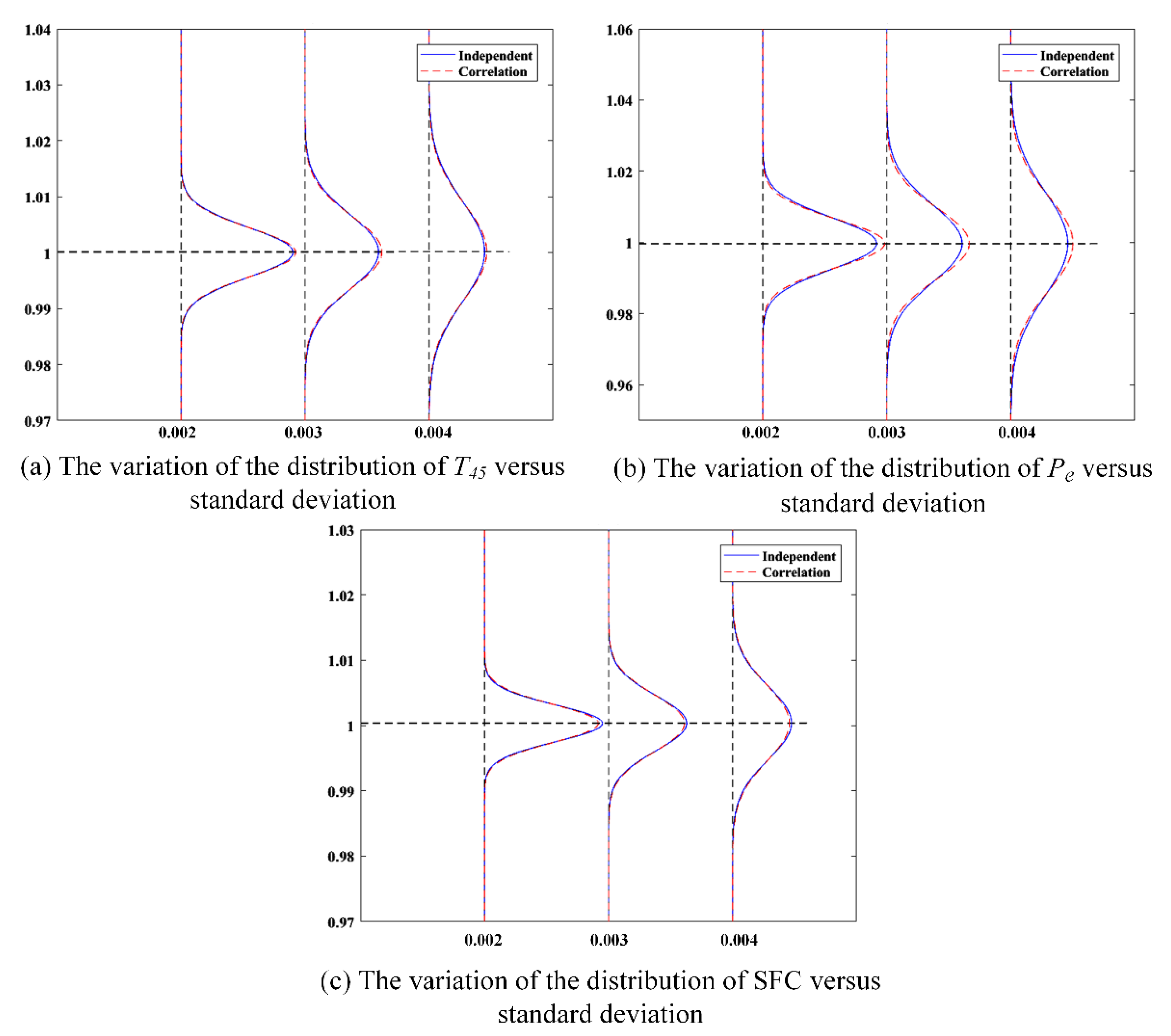
To illustrate the rationality of the independence assumption, two specific scenarios are compared in this section. The first one is that six uncertain parameters are mutually independent, and the other one is that correlations between some uncertain parameters are considered. For the first scenario, six uncertain parameters are assumed to be independent identically distributed. As for the second scenario, a strong correlation between the flow capacity and the adiabatic efficiency of the compressor is additionally assumed, whereas the flow capacity and adiabatic efficiency of the HPT and the LPT are still independent. In each scenario, the uncertain parameters follow the truncated Gaussian distribution with zero mean. Three different standard deviations, i.e., 0.002, 0.003, and 0.004, are considered to investigate the impact of the uncertain parameters. In addition, a correlation efficiency of 60% is specified to represent the correlation between the flow capacity and adiabatic efficiency of the compressor in the second scenario. Thus, a joint Gaussian distribution regarding the two uncertain parameters is generated. Under these assumptions, the distributions of three PMs in each case are predicted through the validated GPM-based LHS method. The results are presented in Figure 5. The blue solid lines represent the distributions of the PMs obtained under the assumption of independence, while the red dashed lines represent those obtained by considering the correlation of partial parameters. It should be noted that the mean and variance of the distribution are predicted by their mean estimates. It can be observed that there is no significant difference in mean estimates between the two cases and the difference is negligible. This can also be found from the summarized results in Table 5. The maximum relative deviation is only 0.003923%. However, the correlation between flow capacity and adiabatic efficiency of the compressor has an impact on the standard deviations of the PMs, especially for the output power . The standard deviation of changes by around 6.6–8.7% as the standard deviation of the uncertain parameters varies within given ranges. As for the other two PMs, the change is about 2.3–4.2% for and 3.0–3.7% for SFC. Moreover, it can be observed in Table 5 that the correlation has a negative effect on the standard deviations of and , but a positive effect on that of SFC. In this situation, if the effect of correlation is ignored, the performance scatter of and may be somewhat overestimated and that of SFC be underestimated to some extent. In practice, the correlation largely depends on the design of the compressor. Thus, it is difficult to obtain a specific correlation between the flow capacity and adiabatic efficiency of the compressor in the preliminary design stage of the engine. In this case, one may preliminarily make an assumption about the correlation based on the engineering experience or directly assume that the parameters are independent of each other. Since the effect of correlation appears weak, the assumption of independence can be acceptable in the early design of the engine.
4.3.3. Uncertainty Analysis of the Turboshaft Engine Performance
In this section, the effects of six uncertain parameters on three PMs of the turboshaft engine is analyzed considering the independence assumption of the parameters. As presented in Figure 5, an apparent phenomenon is that the scatter of each PM becomes larger as the standard deviations of the uncertain parameters increase. In this paper, the performance scatter is defined as six times the standard deviation of the PM, which corresponds to the range of the PM distribution. The -quantile can be approximated as the maximum (positive and negative) deviations from the nominal design value of the PM since the mean value of the PM distribution is very close to the design value. From Table 5, it can be found that the uncertain parameters have a larger influence on than on as well as SFC. Specifically, when the standard deviations of the uncertain parameters is set to the low level (0.002), the performance scatter of is 0.04348, whereas those of and SFC are 0.02653 and 0.01678, respectively. Furthermore, the performance scatters almost double when the standard deviations of the uncertain parameters increase to the high level (0.004). For turboshaft engine designers, the minimum , maximum , and maximum SFC are three important performance indices that need to be paid attention to in the overall performance design. The results of this study indicate that the uncertainties (standard deviation of 0.002) in the component performance may lead to a 1.3% increase in , a 0.84% increase in SFC, and a 2.2% decrease in . These deviations nearly double as the uncertainties become greater (standard deviation of 0.004). Therefore, the engine designers should reserve sufficient performance margins for engine performance (, , and SFC) to compensate for the effect of the component performance uncertainty.
4.4. Sensitivity Analysis of the Turboshaft Engine Performance
After analyzing the engine performance uncertainty, a next important task is to explain the contributions of the uncertain parameters to the performance uncertainties of the PMs and determine the important uncertain parameters. To this end, a variance-based sensitivity analysis which is described in Section 3.3 is implemented for each PM. In this section, all the uncertain parameters are assumed to be independent identically distributed and follow the truncated Gaussian distribution . As demonstrated in Section 3.3, the estimation of the sensitivity index (i.e., ) is mainly affected by the approximation error and sampling error. The former results from the function values predicted by the GPMs and the latter is caused by the finite sample size. Thus, it is essential to firstly investigate the effects of these two kinds of errors.
To investigate the approximation error, the sample size n in the formula of is set to 20,000. For each sample, the distributions of three PMs are predicted by using the built GPMs. Moreover, for each predicted distribution, 100 samples are sampled. Note that all the sampling are based on the LHS method. Figure 6 presents the boxplots of the first-order sensitivity indices of six uncertain parameters. The first-order sensitivity indices of six uncertain parameters are denoted as , , , , , and , which corresponds to the order of the parameters in Table 3. This study focuses on the first-order sensitivity index since the first-order sensitivity indices of six uncertain parameters can account for almost 100% of the total variability in each PM, which will be illustrated in the following analysis. As shown in Figure 6, the variation of each sensitivity index is so small that it can be negligible in this study. It also shows the interquartile range for each boxplot, which is displayed above the corresponding boxplot. The small interquartile ranges indicate that the approximation error has a very weak effect on the sensitivity indices.
To analyze the sampling error, the mean values and the standard deviations of the sensitivity index under different sample size n are compared, ignoring the effect of the approximation error. The sample size varies from 2000 to 20,000 with a step of 2000. To estimate the mean value and standard deviation, the calculation of sensitivity indices is repeated 30 times for each sample size. The mean estimates of sensitivity indices with respect to sample size are presented in Figure 7a,c,e. It can be seen that the mean estimates do not change much when the sample size increases from 2000 to 20,000. Thus, mean estimate of sensitivity index is insensitive to the sample size. Since the mean estimate predominantly reduces the influence of sampling error, it can be adopted to perform sensitivity analysis for the three PMs of the turboshaft engine. In Figure 7b,d,f, a significant decrease in standard deviations can be clearly observed as the sample size increases, which means the sample error can be significantly reduced by taking a large sample size. Eventually, the sample size is chosen as 20,000 and the mean value of is used to estimate the sensitivity index.
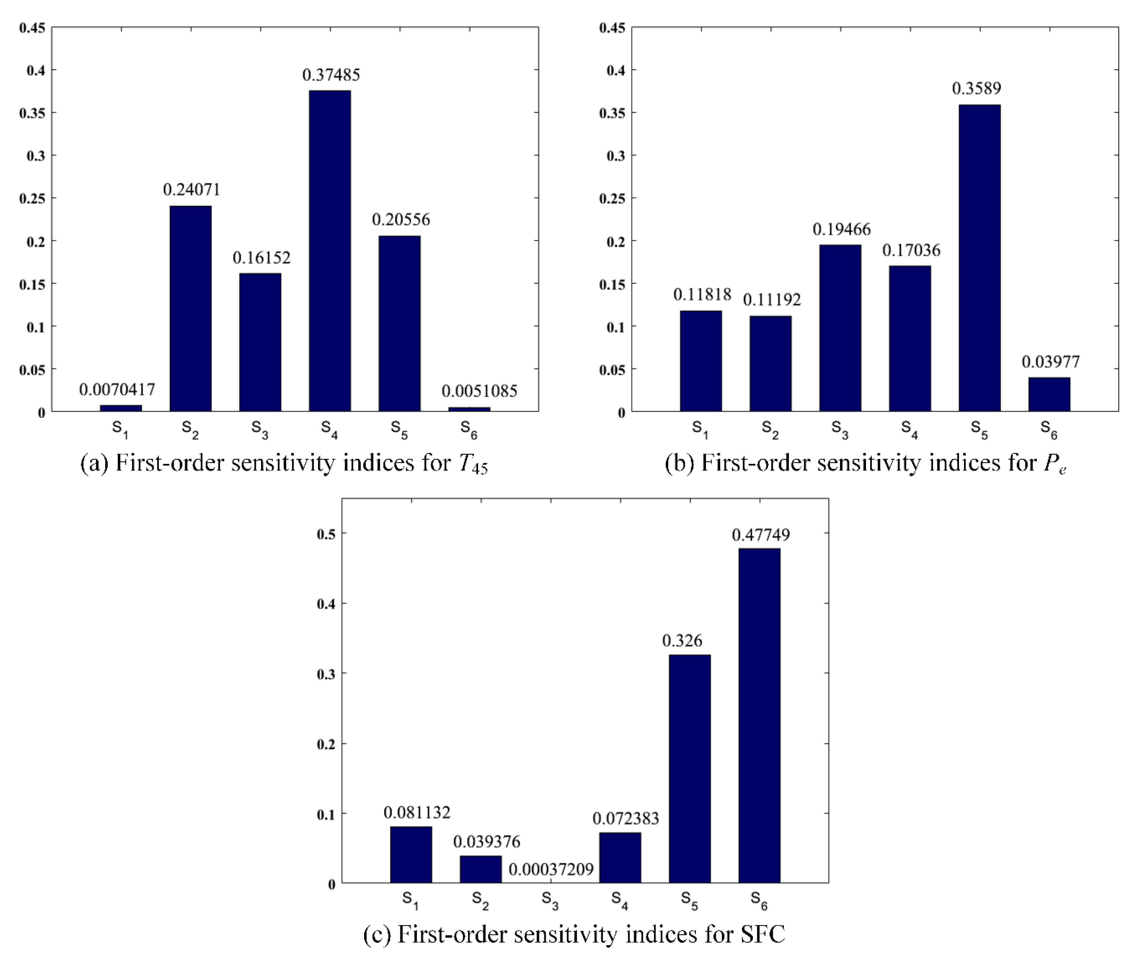
The final sensitivity analysis results for the turboshaft engine performance are shown in Figure 8. It should be noted that the value of each sensitivity index is marked above the corresponding bar. The first-order sensitivity indices of six uncertain parameters nearly account for 100% of the total variabilities of the three PMs, more specifically, 99.48% of the total variability in , 99.38% of the total variability in , and 99.68% of the total variability in SFC. Only a very small proportion of total variability is attributed to the sum of high-order sensitivity indices. The results imply that the main effects of six uncertain parameters have much larger influence on the PMs than the interaction effects do. Recall that , , , , , and denote the first-order sensitivity indices of flow capacity of the compressor (), adiabatic efficiency of the compressor (), flow capacity of the HPT (), adiabatic efficiency of the HPT (), flow capacity of the LPT (), and adiabatic efficiency of the LPT (), respectively. From Figure 8, it can be observed that the six parameters play different roles in the three PMs. For , is the most important parameter, which accounts for 37.485% of the total variability in . In the meantime, , , and are also important to as their indices are all greater than 10%. In particular, and are found to have little effect on due to their small indices (). For , has the most important effect on comparing to other parameters since it contributes the highest percentage (35.89%) of the total variability in . The rest of the parameters except are all considered as important parameters for since the sum of their indices are about 60% and each index exceeds 10%. By contrast, is less important to . As for SFC, there are two most important parameters ( and ) due to their large indices. The remaining four parameters are relatively unimportant to SFC. It should be noticed that has, particularly, almost no effect on SFC.
5. Conclusions
The demand for quantifying the uncertainty of engine performance in the preliminary design is increasing due to the expectation of reliable engine performance design. In this paper, a GPM-based uncertainty quantification method is proposed to quantify the effect of component performance uncertainty on the overall performance of a turboshaft engine. Six uncertain parameters related to the component performance and three PMs of the engine are determined. To significantly reduce the number of running the time-consuming simulation model, three GPMs that reflect the functional relationships between six uncertain parameters and three PMs are constructed. The validation shows that the GPMs are of high accuracy. LHS is utilized to propagate the uncertainty to the engine performance and provide the statistical information of the engine performance. The GPM-based LHS is validated to perform better than the most frequently used simulation-based MCS. In addition, based on the GPMs, the variance-based sensitivity analysis is employed to recognize the main contributors to the engine performance uncertainty. According to the first-order sensitivity index, the important uncertain parameters for three PMs are determined with the criterion , which is very useful for the engine designers. To obtain reliable and robust results, both approximation and sampling errors are investigated in this study. Some useful results are summarized as follows:
- (1)
- A strong correlation (with a correlation efficiency of 60%) between the flow capacity and adiabatic efficiency of compressor only has a small influence on the standard deviation of the turboshaft engine performance. Specifically, the standard deviation of decreases by around 6.6–8.7% as the standard deviation of uncertain parameters varies from 0.002 to 0.004. Likewise, a reduction of 2.3–4.2% is observed for , but an increase of 3.0–3.7% for SFC.With an assumption of independent parameters, the maximum , minimum , and maximum SFC deviate 1.3%, 2.2%, and 0.84% from their nominal design values in the unfavorable direction when the standard deviations of uncertain parameters are equal to 0.002. The deviations almost double as the standard deviations increase to 0.004.
- (2)
- The first-order sensitivity indices of six uncertain parameters almost account for 100% of the total variabilities of the three PMs, more specifically, 99.48% of the total variability in , 99.38% of the total variability in , and 99.68% of the total variability in SFC. Only a very small proportion of total variability is attributed to the sum of high-order sensitivity indices.
- (3)
- The important parameters for are , , , and . All the uncertain parameters other than are the important parameters for . Only and are the important parameters for SFC. In particular, is important to all the three PMs of the turboshaft engine.
Author Contributions
Conceptualization, X.L., H.T. and X.Z.; methodology, X.L.; software, X.L.; validation, X.L. and X.Z.; formal analysis, X.L.; investigation, X.L. and X.Z.; resources, X.L. and X.Z.; data curation, X.L.; writing—original draft preparation, X.L.; writing—review and editing, H.T. and M.C.; visualization, X.L.; supervision, H.T. and M.C.; project administration, H.T. and M.C.; funding acquisition, H.T. and M.C. All authors have read and agreed to the published version of the manuscript.
Funding
This research was funded by National Natural Science Foundation of China, grant number 51776010 and 91860205.
Institutional Review Board Statement
Not applicable.
Informed Consent Statement
Not applicable.
Data Availability Statement
The data presented in this study are available on request from the corresponding author. The data are not publicly available due to the intellectual property rights.
Acknowledgments
The authors are thankful for the support from Collaborative Innovation Center of Advanced Aero-Engine.
Conflicts of Interest
The authors declare no conflict of interest.
References
- Kurzke, J.; Halliwell, I. Propulsion and Power; Springer: Cham, Switzerland, 2018; pp. 5–42. [Google Scholar] [CrossRef]
- Giampaolo, T. Gas Turbine Handbook: Principles and Practice, 5th ed.; The Fairmont Press: Lilburn, GA, USA, 2014; pp. 45–77. [Google Scholar]
- Garzon, V.E.; Darmofal, D.L. Impact of Geometric Variability on Axial Compressor Performance. J. Turbomach. 2003, 125, 1199–1213. [Google Scholar] [CrossRef] [Green Version]
- Lange, A.; Voigt, M.; Vogeler, K.; Johann, E. Principal component analysis on 3D scanned compressor blades for probabilistic CFD simulation. In Proceedings of the 53rd AIAA/ASME/ASCE/AHS/ASC Structures, Structural Dynamics and Materials Conference, Honolulu, HI, USA, 23–26 April 2012. [Google Scholar] [CrossRef]
- Spieler, S.; Staudacher, S.; Fiola, R.; Sahm, P.; Weißschuh, M. Probabilistic engine performance scatter and deterioration modeling. J. Eng. Gas. Turbines Power 2008, 130, 150–158. [Google Scholar] [CrossRef]
- Zhang, J.Y.; Tang, H.L.; Chen, M. Linear substitute model-based uncertainty analysis of complicated non-linear energy system performance (case study of an adaptive cycle engine). Appl. Energy 2019, 249, 87–108. [Google Scholar] [CrossRef]
- Chen, M.; Zhang, K.; Tang, H.L. A Probabilistic Design Methodology for a Turboshaft Engine Overall Performance Analysis. Adv. Mech. Eng. 2014, 8, 1–12. [Google Scholar] [CrossRef] [Green Version]
- Cao, D.; Bai, G. A Study on Aeroengine Conceptual Design Considering Multi-Mission Performance Reliability. Appl. Sci. 2020, 10, 46–68. [Google Scholar] [CrossRef]
- Tai, J.C.M.; Mines, J.M.; Inclan, E.; Zhu, S.; Mavris, D.N. Uncertainty Quantification and Management in Engine Conceptual Design. In Proceedings of the 52nd AIAA/SAE/ASEE Joint Propulsion Conference, Salt Lake City, UT, USA, 25–27 July 2016. [Google Scholar] [CrossRef]
- Lamorte, N.; Friedmann, P.P.; Dalle, D.J.; Torrez, S.M.; Driscoll, J.F. Uncertainty Propagation in Integrated Airframe–Propulsion System Analysis for Hypersonic Vehicles. J. Propul. Power 2015, 31, 1–15. [Google Scholar] [CrossRef] [Green Version]
- Zheng, J.; Chang, J.; Ma, J.; Yu, D. Performance uncertainty propagation analysis for control-oriented model of a turbine-based combined cycle engine. Acta Astronaut. 2018, 153, 39–49. [Google Scholar] [CrossRef]
- Montomoli, F. Uncertainty Quantification in Computational Fluid Dynamics and Aircraft Engines; Springer: Cham, Switzerland, 2019; pp. 80–82. [Google Scholar] [CrossRef]
- Chen, M.; Zhang, J.; Tang, H. Interval analysis of the standard of adaptive cycle engine component performance deviation. Aerosp. Sci. Technol. 2018, 81, 179–191. [Google Scholar] [CrossRef]
- Fu, C.; Xu, Y.; Yang, Y.; Lu, K.; Gu, F.; Ball, A. Response analysis of an accelerating unbalanced rotating system with both random and interval variables. J. Sound Vib. 2019, 466. [Google Scholar] [CrossRef]
- Helton, J.C.; Johnsom, J.D.; Sallaberry, C.J.; Storlie, C.B. Survey of sampling-based methods for uncertainty and sensitivity analysis. Reliab. Eng. Syst. Saf. 2006, 91, 1175–1209. [Google Scholar] [CrossRef] [Green Version]
- Davis, J.C.; Helton, F.J. Latin hypercube sampling and the propagation of uncertainty in analyses of complex systems. Reliab. Eng. Syst. Saf. 2003, 81, 23–69. [Google Scholar] [CrossRef] [Green Version]
- Sacks, J.; Welch, W.J.; Mitchell, T.J.; Wynn, H.P. Design and analysis of computer experiments. Stat. Sci. 1989, 4, 409–423. [Google Scholar] [CrossRef]
- Currin, C.; Mitchell, T.; Morris, M.; Ylvisaker, D. Bayesian prediction of deterministic functions, with applications to the design and analysis of computer experiments. J. Am. Stat. Assoc. 1991, 86, 953–963. [Google Scholar] [CrossRef]
- Santner, T.J.; Williams, B.J.; Notz, W.I. The Design and Analysis of Computer Experiments; Springer: New York, NY, USA, 2003; pp. 1–3, 27–37. [Google Scholar]
- Chapman, J.W.; Lavelle, T.M.; May, R.; Litt, J.S.; Guo, T.H. Propulsion System Simulation Using the Toolbox for the Modeling and Analysis of Thermodynamic Systems (T-MATS). In Proceedings of the 50th AIAA/SAE/ASEE Joint Propulsion Conference, Cleveland, OH, USA, 28–30 July 2014. [Google Scholar] [CrossRef] [Green Version]
- Chapman, J.W.; Lavelle, T.M.; Litt, J.S. Practical techniques for modeling gas turbine engine performance. In Proceedings of the 52nd AIAA/SAE/ASEE Joint Propulsion Conference, Salt Lake City, UT, USA, 25–27 July 2016. [Google Scholar] [CrossRef] [Green Version]
- Al-Hamdan, Q.Z.; Ebaid, M.S.Y. Modeling and Simulation of a Gas Turbine Engine for Power Generation. J. Eng. Gas. Turbines Power 2006, 128, 302–311. [Google Scholar] [CrossRef]
- Chen, M.; Tang, H.L.; Zhu, Z.L. Goal Programming for Stable Mode Transition in Tandem Turbo-ramjet Engine. Chin. J. Aeronaut. 2009, 22, 486–492. [Google Scholar] [CrossRef] [Green Version]
- Tang, H.L.; Chen, M.; Jin, D.H.; Zou, Z.P. High altitude low Reynolds number effect on the matching performance of a turbofan engine. Proc. Inst. Mech. Eng. Part G-J. Aerosp. Eng. 2013, 227, 455–466. [Google Scholar] [CrossRef]
- Chen, M.; Tang, H.L.; Zhang, K.; Hui, O.Y.; Wang, Y.J. Turbine-based combined cycle propulsion system integration concept design. Proc. Inst. Mech. Eng. Part G-J. Aerosp. Eng. 2012, 227, 1068–1089. [Google Scholar] [CrossRef]
- Zheng, J.C.; Tang, H.L.; Chen, M.; Yin, F.J. Equilibrium running principle analysis on an adaptive cycle engine. Appl. Therm. Eng. 2018, 132, 393–409. [Google Scholar] [CrossRef] [Green Version]
- Ghani, F.; Fernandez, E.F.; Almonacid, F.; O’Donovan, T.S. The numerical computation of lumped parameter values using the multi-dimensional Newton-Raphson method for the characterisation of a multi-junction CPV module using the five-parameter approach. Sol. Energy 2017, 149, 302–313. [Google Scholar] [CrossRef]
- Rasmussen, C.E.; Williams, C.K.I. Gaussian Processes for Machine Learning; MIT Press: Cambridge, UK, 2005; pp. 81–83. [Google Scholar] [CrossRef] [Green Version]
- Marrel, A.; Iooss, B.; Laurent, B.; Roustant, O. Calculations of sobol indices for the Gaussian process metamodel. Reliab. Eng. Syst. Saf. 2008, 94, 742–751. [Google Scholar] [CrossRef] [Green Version]
- Tan, M.H.Y. Robust Parameter design with computer experiments using orthonormal polynomials. Technometrics 2015, 57, 468–478. [Google Scholar] [CrossRef]
- Roshanian, J.; Ebrahimi, M. Latin hypercube sampling applied to reliability-based multidisciplinary design optimization of a launch vehicle. Aerosp. Sci. Technol. 2013, 28, 297–304. [Google Scholar] [CrossRef]
- Mckay, M.D.; Conover, W.J.; Beckman, R.J. A Comparison of Three Methods for Selecting Values of Input Variables in the Analysis of Output from a Computer Code. Technometrics 1979, 21, 239–245. [Google Scholar] [CrossRef]
- Sobol, I.M. Sensitivity analysis for nonlinear mathematical models. Math. Model. Comput. Exp. 1993, 1, 407–414. [Google Scholar]
- Sobol, I.M. Global sensitivity indices for nonlinear mathematical models and their Monte Carlo estimates. Math. Comput. Simul. 2001, 55, 271–280. [Google Scholar] [CrossRef]
- Oakley, J.E.; O’Hagan, A. Probabilistic sensitivity analysis of complex models: A Bayesian approach. J. R. Stat. Soc. Ser. B Stat. Methodol. 2004, 66, 751–769. [Google Scholar] [CrossRef] [Green Version]
- Janon, A.; Klein, T.; Lagnoux, A.; Nodet, M. Asymptotic normality and efficiency of two Sobol index estimators. ESAIM Prob. Stat. 2014, 18, 342–364. [Google Scholar] [CrossRef] [Green Version]
- Naeem, M.; Singh, R.; Probert, D. Consequences of aero-engine deteriorations for military aircraft. Appl. Energy 2001, 70, 103–133. [Google Scholar] [CrossRef]
- Brown, H.; Elgin, J.A. Aircraft Engine Control Mode Analysis. J. Eng. Gas. Turbines Power 1985, 107, 838–844. [Google Scholar] [CrossRef]
- Loeppky, J.L.; Sacks, J.; Welch, W.J. Choosing the sample size of a computer experiment: A practical guide. Technometrics 2009, 51, 366–376. [Google Scholar] [CrossRef] [Green Version]
Figure 1.
The configuration of the turboshaft engine.
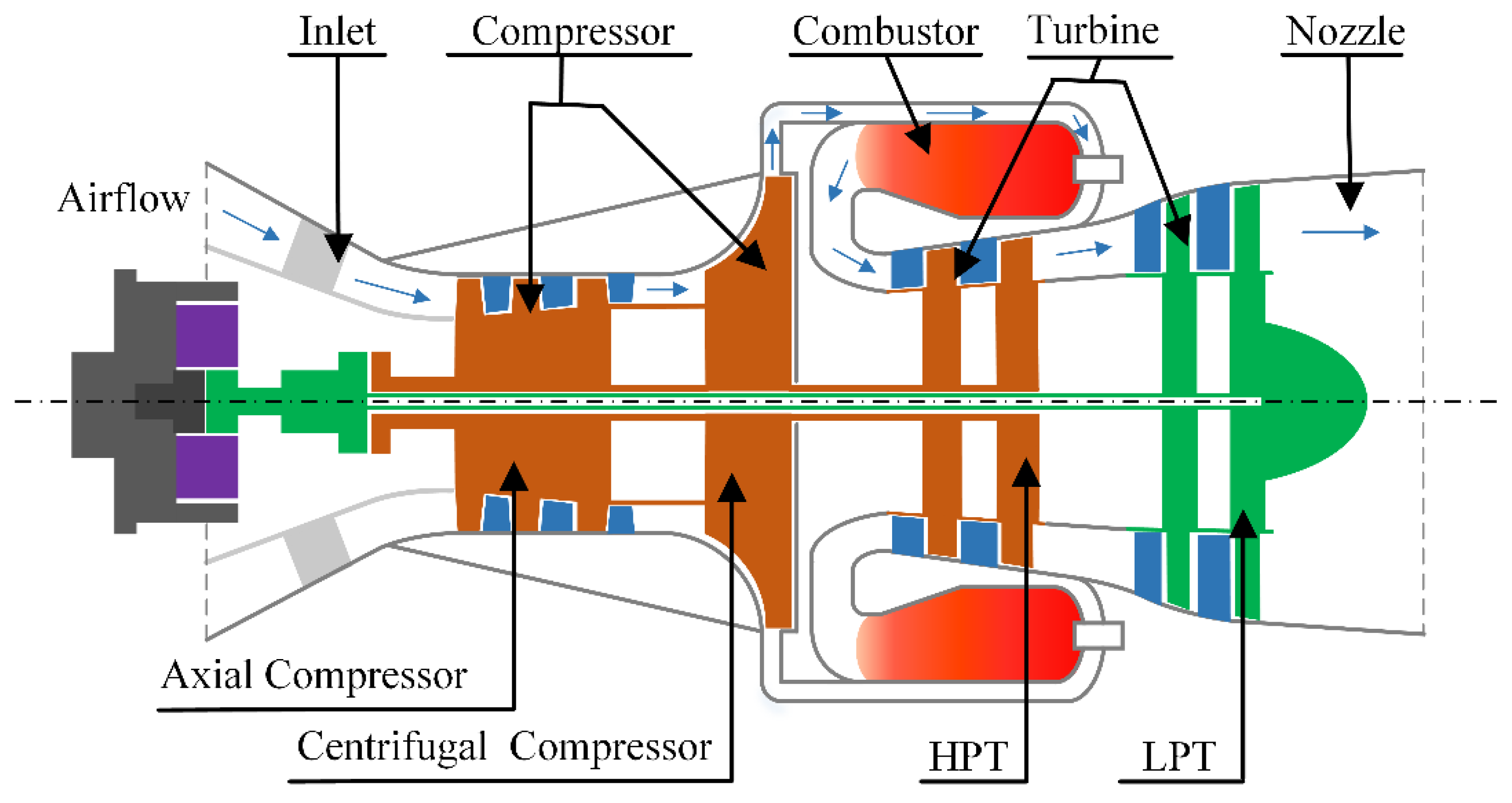
Figure 2.
(a) The pressure ratio–corrected mass flow map; (b) the adiabatic efficiency–corrected mass flow map.
Figure 2.
(a) The pressure ratio–corrected mass flow map; (b) the adiabatic efficiency–corrected mass flow map.
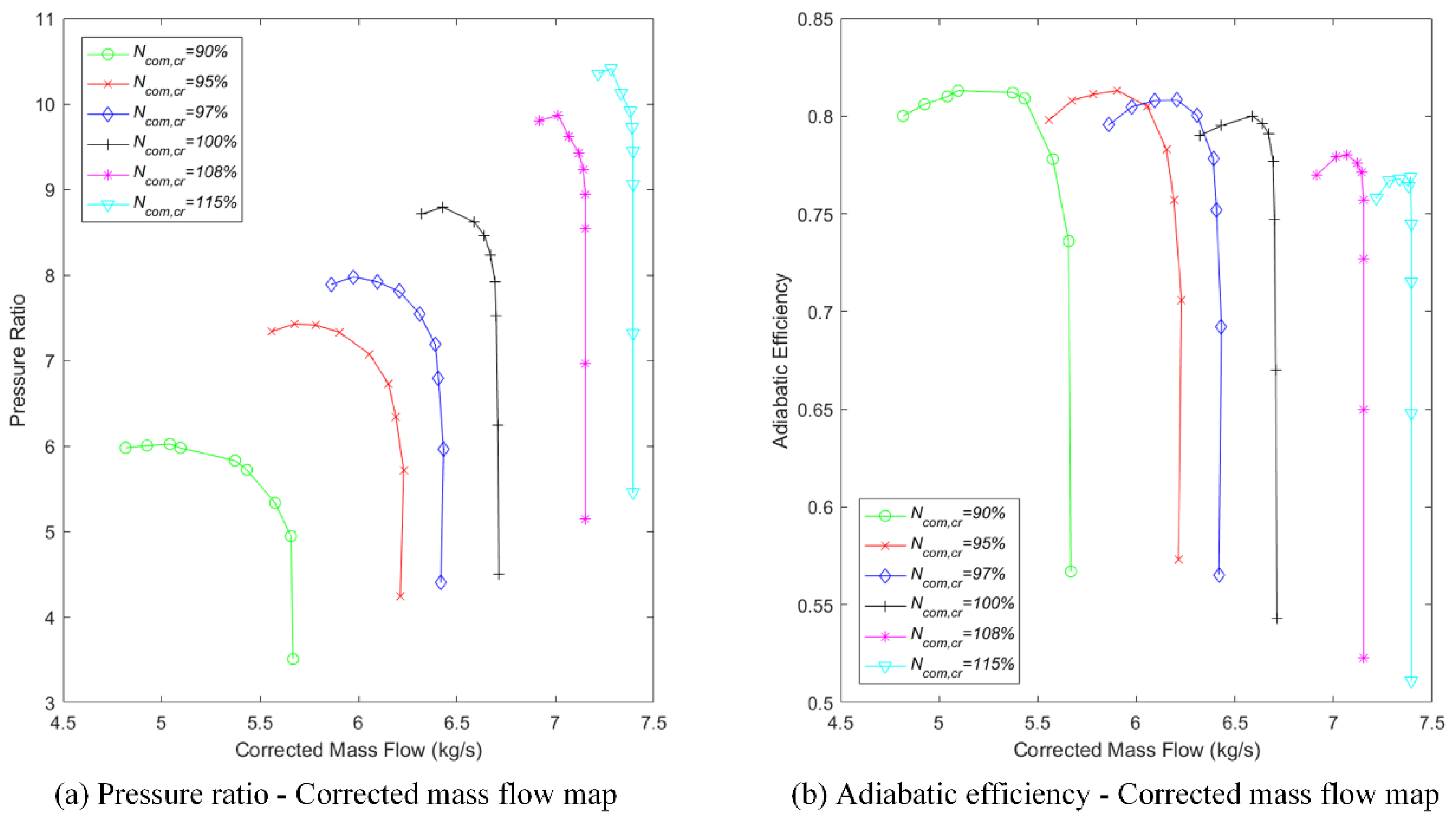
Figure 3.
(a) The boxplots of NRMSE for against Latin hypercube design (LHD) size; (b) the boxplots of for against LHD size; (c) the boxplots of NRMSE for against LHD size; (d) the boxplots of for against LHD size; (e) the boxplots of NRMSE for specific fuel consumption (SFC) against LHD size; (f) the boxplots of for SFC against LHD size.
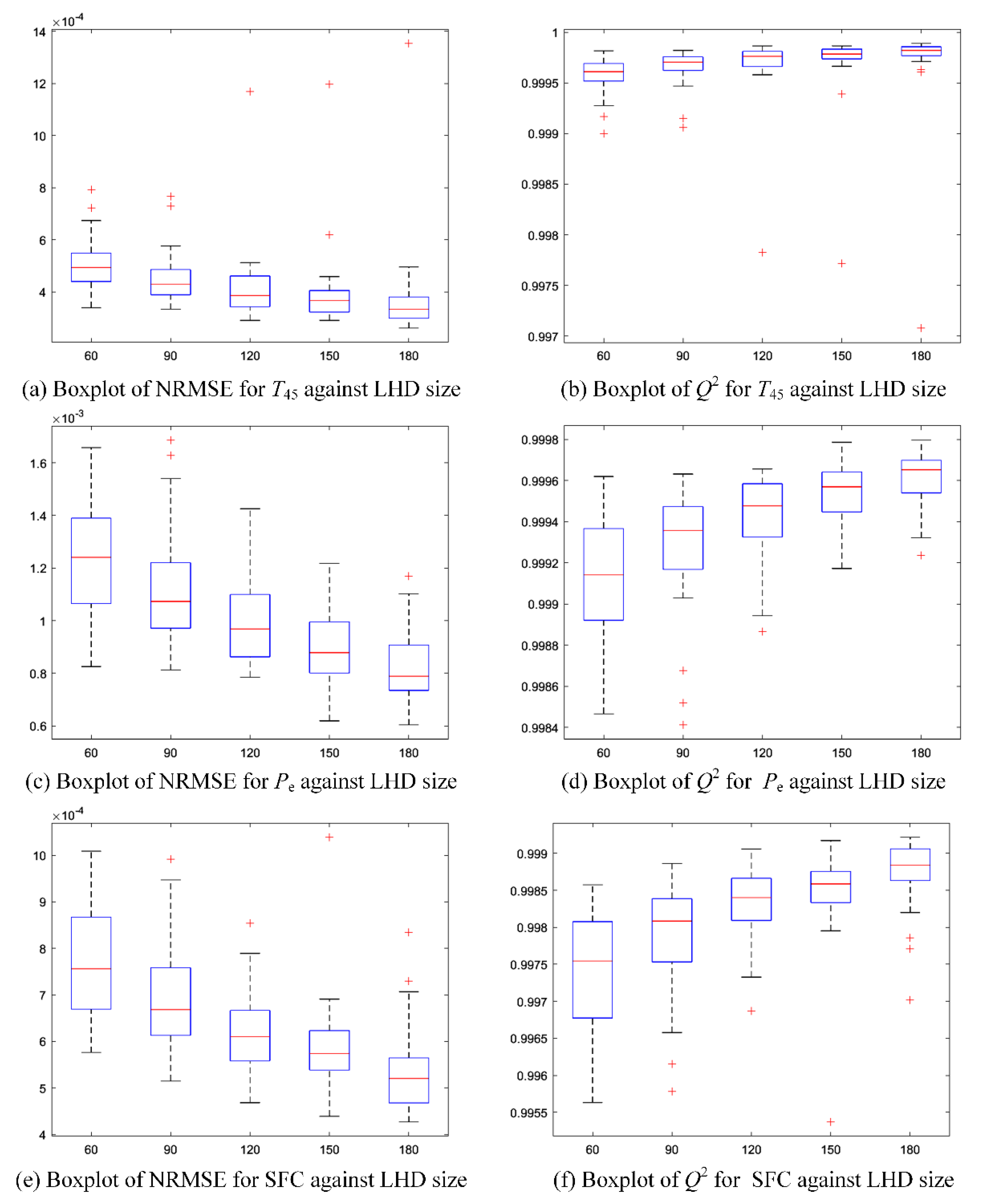
Figure 4.
(a) Mean of versus sample size; (b) variance of versus sample size; (c) mean of versus sample size; (d) variance of versus sample size; (e) mean of SFC versus sample size; (f) variance of SFC versus sample size.
Figure 4.
(a) Mean of versus sample size; (b) variance of versus sample size; (c) mean of versus sample size; (d) variance of versus sample size; (e) mean of SFC versus sample size; (f) variance of SFC versus sample size.
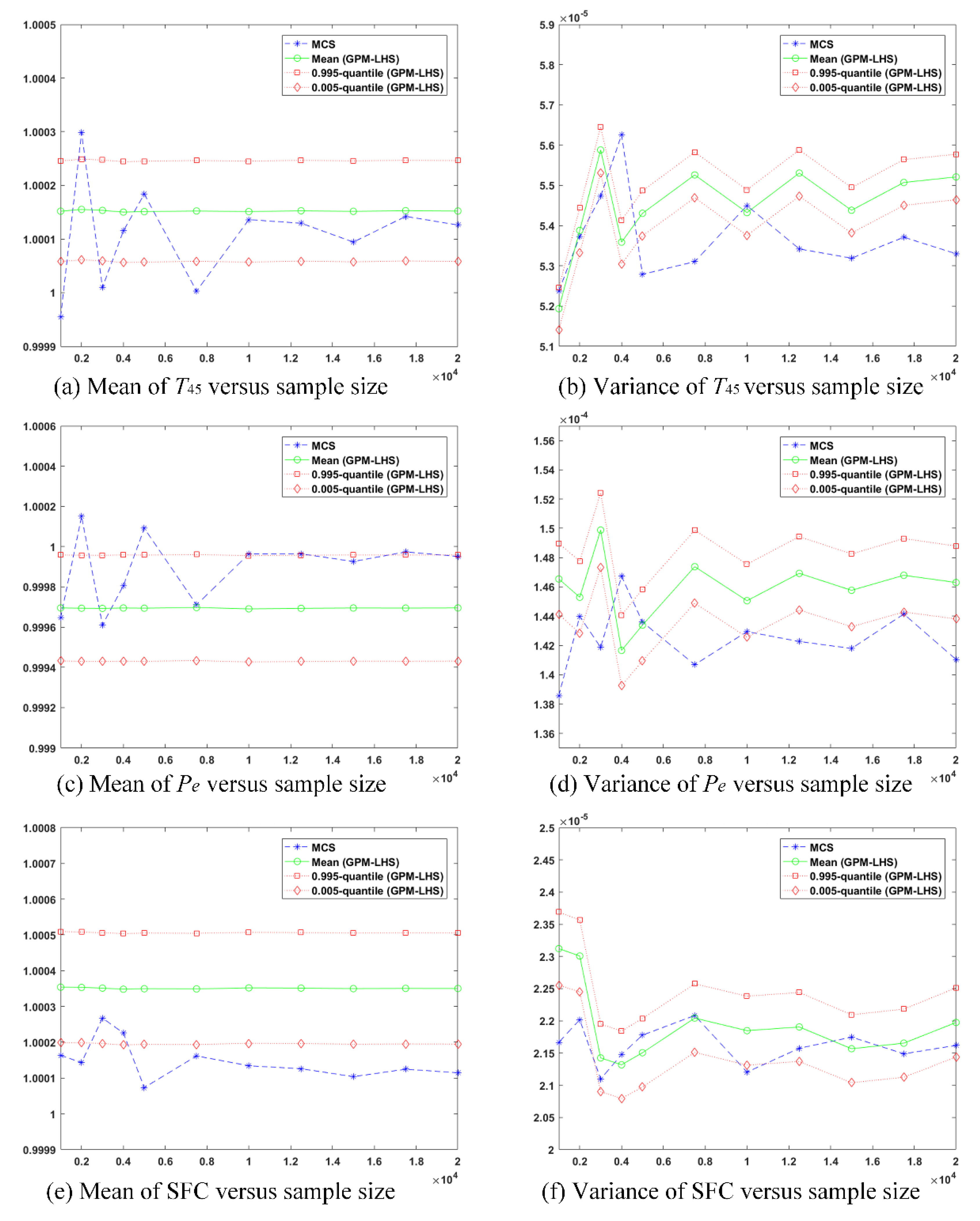
Figure 5.
(a) The variation of the distribution of versus standard deviations of the six uncertain parameters; (b) the variation of the distribution of versus standard deviations of the six uncertain parameters; (c) the variation of the distribution of SFC versus standard deviations of the six uncertain parameters.

Figure 6.
(a) The boxplot of first-order sensitivity index for ; (b) the boxplot of first-order sensitivity index for ; (c) the boxplot of first-order sensitivity index for SFC (the value above each boxplot represents corresponding the interquartile range).
Figure 6.
(a) The boxplot of first-order sensitivity index for ; (b) the boxplot of first-order sensitivity index for ; (c) the boxplot of first-order sensitivity index for SFC (the value above each boxplot represents corresponding the interquartile range).
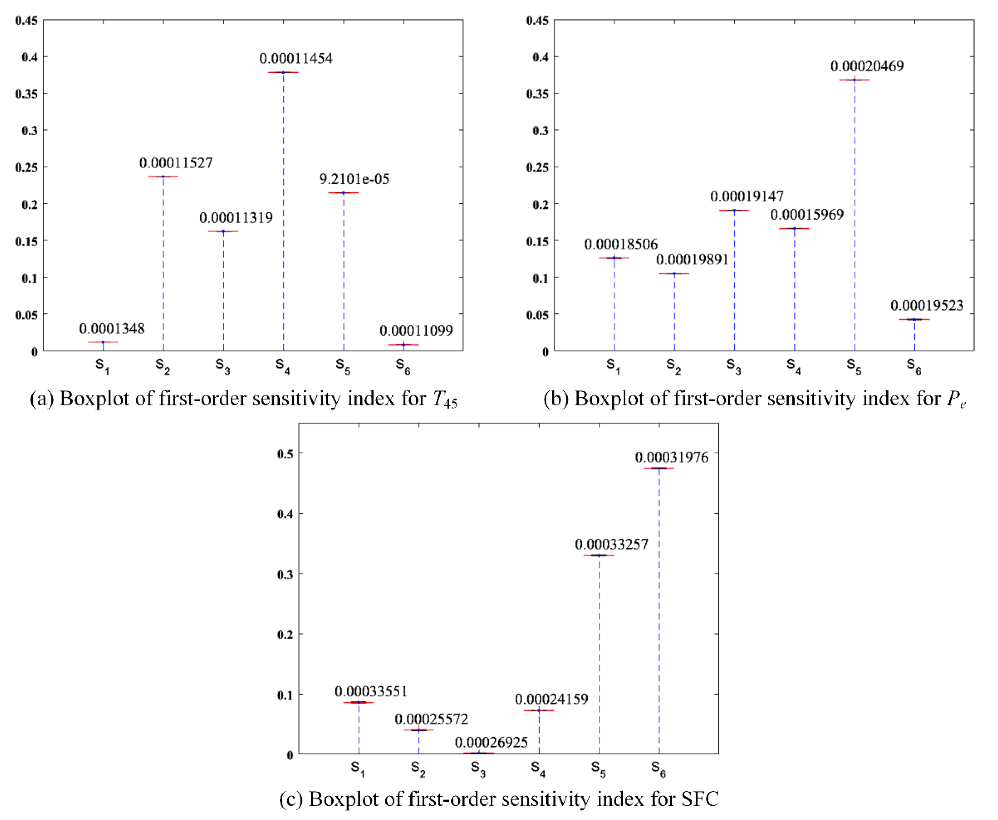
Figure 7.
(a) The mean values of sensitivity indices of six uncertain parameters for versus sample size; (b) the standard deviations of sensitivity indices of six uncertain parameters for versus sample size; (c) the mean values of sensitivity indices of six uncertain parameters for versus sample size; (d) the standard deviations of sensitivity indices of six uncertain parameters for versus sample size; (e) the mean values of sensitivity indices of six uncertain parameters for SFC versus sample size; (f) the standard deviations of sensitivity indices of six uncertain parameters for SFC versus sample size.

Figure 8.
(a) The first-order sensitivity indices of six uncertain parameters for ; (b) the first-order sensitivity indices of six uncertain parameters for ; (c) the first-order sensitivity indices of six uncertain parameters for SFC (the value above each boxplot represents corresponding the interquartile range).

Table 1.
The undetermined parameters in the simulation model.
| No. | Notation | Undetermined Parameters |
|---|---|---|
| 1 | The location of the operating point of compressor | |
| 2 | The location of the operating point of HPT | |
| 3 | The location of the operating point of LPT | |
| 4 | The fuel flow |
Table 2.
The ambient conditions, working conditions, and control variables.
| Parameter | Value | Unit |
|---|---|---|
| Ambient temperature | 288.15 | K |
| Ambient pressure | 101,325 | Pa |
| Height | 0 | km |
| Mach number | 0 | -- |
| Relative spool speed of HPR (control variable) | 0.97 | -- |
| Relative spool speed of LPT (control variable) | 1 | -- |
Table 3.
The description of the uncertain parameters.
| Component | Uncertain Parameter | Notation | High Level | Low Level | Probabilistic Distribution |
|---|---|---|---|---|---|
| Compressor | Flow capacity | 0.02 | −0.02 | Truncated Gaussian distribution | |
| Adiabatic efficiency | 0.02 | −0.02 | Truncated Gaussian distribution | ||
| HPT | Flow capacity | 0.02 | −0.02 | Truncated Gaussian distribution | |
| Adiabatic efficiency | 0.02 | −0.02 | Truncated Gaussian distribution | ||
| LPT | Flow capacity | 0.02 | −0.02 | Truncated Gaussian distribution | |
| Adiabatic efficiency | 0.02 | −0.02 | Truncated Gaussian distribution |
Table 4.
Mean values of NRMSE and for GPMs of three PMs obtained by 30 LHD replications for each size in .
Table 4.
Mean values of NRMSE and for GPMs of three PMs obtained by 30 LHD replications for each size in .
| LHD Size | T45 | Pe | SFC | |||
|---|---|---|---|---|---|---|
| NRMSE | Q2 | NRMSE | Q2 | NRMSE | Q2 | |
| 60 | 0.000508 | 0.999573 | 0.001237 | 0.999121 | 0.000761 | 0.997458 |
| 90 | 0.000451 | 0.99966 | 0.001118 | 0.999278 | 0.000696 | 0.997864 |
| 120 | 0.000417 | 0.999686 | 0.000999 | 0.999427 | 0.000620 | 0.998322 |
| 150 | 0.000398 | 0.999705 | 0.000900 | 0.999536 | 0.00059 | 0.998464 |
| 180 | 0.000378 | 0.999715 | 0.000826 | 0.999609 | 0.000538 | 0.998723 |
Table 5.
The relative deviations between the two scenarios for three PMs under different standard deviations of the uncertain parameters.
Table 5.
The relative deviations between the two scenarios for three PMs under different standard deviations of the uncertain parameters.
| Performance Parameters | Distribution Parameters | Relative Deviation (σ = 0.002) | Relative Deviation (σ = 0.003) | Relative Deviation (σ = 0.004) |
|---|---|---|---|---|
| T45 | Mean | −0.000175% | −0.000876% | −0.001247% |
| Std * | −2.337830% | −4.218916% | −3.548779% | |
| Pe | Mean | 0.001091% | 0.002451% | 0.003923% |
| Std * | −6.624252% | −8.693671% | −8.350732% | |
| SFC | Mean | −0.000679% | −0.001874% | −0.003072% |
| Std * | 3.716896% | 2.997669% | 3.738209% |
* Std denotes the standard deviation of the parameter.
Publisher’s Note: MDPI stays neutral with regard to jurisdictional claims in published maps and institutional affiliations. |
© 2021 by the authors. Licensee MDPI, Basel, Switzerland. This article is an open access article distributed under the terms and conditions of the Creative Commons Attribution (CC BY) license (https://creativecommons.org/licenses/by/4.0/).
Share and Cite
MDPI and ACS Style
Liu, X.; Tang, H.; Zhang, X.; Chen, M. Gaussian Process Model-Based Performance Uncertainty Quantification of a Typical Turboshaft Engine. Appl. Sci. 2021, 11, 8333. https://doi.org/10.3390/app11188333
AMA Style
Liu X, Tang H, Zhang X, Chen M. Gaussian Process Model-Based Performance Uncertainty Quantification of a Typical Turboshaft Engine. Applied Sciences. 2021; 11(18):8333. https://doi.org/10.3390/app11188333
Chicago/Turabian StyleLiu, Xuejun, Hailong Tang, Xin Zhang, and Min Chen. 2021. "Gaussian Process Model-Based Performance Uncertainty Quantification of a Typical Turboshaft Engine" Applied Sciences 11, no. 18: 8333. https://doi.org/10.3390/app11188333
Note that from the first issue of 2016, this journal uses article numbers instead of page numbers. See further details here.