
Multiparameter Determination of Thin Liquid Urea-Water Films


Institute for Reactive Flows and Diagnostics, Technical University of Darmstadt, 64287 Darmstadt, Germany
*
Author to whom correspondence should be addressed.
Appl. Sci. 2021, 11(19), 8925; https://doi.org/10.3390/app11198925
Submission received: 12 August 2021
/
Revised: 20 September 2021
/
Accepted: 21 September 2021
/
Published: 24 September 2021
(This article belongs to the Special Issue Diode Laser Spectroscopy – Robust Sensing for Environmental and Industrial Applications)
Abstract
:In this work, wavelengths were determined for the robust and simultaneous measurement of film thickness, urea concentration and fluid temperature. Film parameters such as film thickness, film temperature and the composition of the film are typically dynamically and interdependently changing. To gain knowledge of these quantities, a measurement method is required that offers a high temporal resolution while being non-intrusive so as to not disturb the film as well as the process conditions. We propose the extension of the FMLAS method, which was previously validated for the film thickness measurement of thin liquid films, to determine temperatures and concentrations using an adapted evaluation approach.
1. Introduction
In many industrial applications, the formation of thin liquid films, whether it be desired or not, has a significant influence on the underlying processes. Examples range from printing or coating processes [1,2] and lubrication purposes [3,4] to the formation of oil films on piston heads, causing pool fires and leading to an increase in pollutants in exhaust gas [5,6]. Another process where film formation has a high relevance is the selective catalytic reduction process (SCR), which is a state-of-the-art method to reduce nitrous oxides from the exhaust gas of diesel engines. A Urea-Water solution (UWS or AdBlue) is injected into the hot exhaust gas stream upstream of the SCR catalyst. Through thermolysis and hydrolysis processes, ammonia is formed, which acts as the reducing agent. However, depending on the operation conditions, a liquid UWS film can form on the surrounding walls, which can subsequently form solid deposits.
In order to comply with the limits of nitrogen oxides in the future, the SCR process must be understood in detail. Film formation, in particular, is a crucial parameter that can lead to a reduction in the efficiency of the SCR [7]. The investigation of the formation of the liquid film and deposit formation on the overall SCR process plays a leading role. Thus, key film parameters, such as film thickness, temperature and concentration of urea in water, must be monitored [8].
A wide range of measurement of non-intrusive methods have been proposed in the past for the determination of film parameters, which include laser-induced fluorescence [9,10], ultrasonic measurements [11,12] and Raman spectroscopy [13,14]. However, among this selection of multiple methods, only laser absorption spectroscopy currently offers the ability to measure film thickness, concentration and temperature of a fluid simultaneously.
In this work, we propose the extension of the film measurement laser absorption spectroscopy (FMLAS) method, which has previously been validated and implemented for film thickness measurements, for the determination of temperatures and concentrations of a thin UWS film [15,16,17]. The FMLAS method provides some significant advantages: it is non-intrusive, allows for a high temporal resolution and has a cost-effective setup based on readily available near-infrared laser diodes. The research presented here prepared for the use of diode lasers by selecting the optimal emission wavelength.
FMLAS is based on the Beer–Lambert–Law for induced absorption:
where the detected light intensity is a function of the incident light and the absorbance at the wavenumber . In turn, is a function of the absorption coefficient and the film parameters of film thickness , concentration and temperature . With the FMLAS approach, can be determined by intensity measurements at two suitable wavenumbers through quotient formation after calibration (see [16]).
The aim of this work is to find optimized wavenumber combinations that allow for the determination of as well as the additional film parameters of and (concentration %mass of urea in water). For this purpose, the broadband transmission spectra of a comprehensive calibration data set are recorded with a Fourier transform infrared (FTIR) spectrometer. In contrast to , the parameters of and exhibit a nonlinear dependency on the absorbance which is why a novel evaluation strategy for the spectral data is additionally required. We introduce an approach to spectroscopically determine the film parameters through an adapted calibration method, which is then used to evaluate a test set. Furthermore, an optimization strategy is presented for the wavenumber selection.
2. Experimental Setup and Methodology
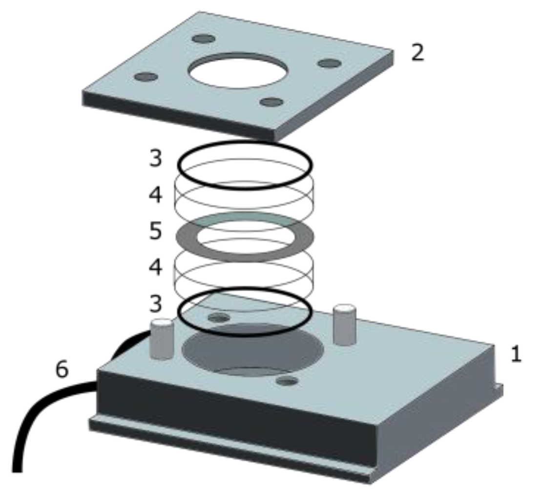
Firstly, the broadband spectra of known film parameters are collected with an FTIR spectrometer (Bruker: VERTEX 80v). Spectra in the wavenumber range from around 2000 cm−1 to 15,000 cm−1 were recorded with a thermoelectrically cooled Indium Gallium Arsenide (TE InGaAs) detector. A calibration cell [16] was used to enable transmission measurements with predefined parameter variations (see Figure 1). The UWS is placed within the stainless steel spacer ring, which is then clamped between two wedged calcium fluoride (CaF2) windows, two O-seals and the top and body plates of the cell. The film thickness is given by the height of the spacer, while the temperature is set through heating cartridges and monitored by a thermocouple. The concentration of the urea in water is known beforehand as it is mixed from solid urea and water.
To enable a reliable calibration, a comprehensive measurement matrix was used comprising 4 concentration variations, 8 temperature variations and 6 film thickness variations (see Table 1). The minimal concentration was set to 32.5%mass, as this corresponds to the commercially available product. Higher concentrations are likely to occur during the SCR process due to the evaporation of water within the hot gas stream, which is why higher concentrations up to 57.7%mass were also investigated. Film thicknesses as low as 91 μm could be realized within the calibration cell, while the use of thinner stainless steel foils proved to be unfeasible. Small burrs at the edges of the foils led to an overestimation of the film thickness. The maximum film thickness within the measurement matrix amounted to 310 μm. The investigated temperatures ranged from room temperature (25 °C) to 30 °C and—in steps of ten degrees—up to 90 °C. All parameter variations were investigated, leading to 192 experiments. However, in some higher temperature cases, bubble formation led to low-quality measurements that had to be discarded. Thus, a total of 160 measurements with different parameter combinations were used for the subsequent evaluation.
In addition to these transmission measurements, background measurements are required, which are taken through the empty calibration cell. Thus, the quantities and are known from the experiments, and the respective absorbance spectra can be calculated with Equation (1). For further evaluation, the absorbance spectra are most suitable since these are independent of the measurement conditions and environment or the detector behavior. This way, data from different campaigns and setups or taken with different detectors can be compared, which would not be possible if the attenuated intensity signal were utilized. Comparing the empty cell (background scan) and filled cell (liquid between windows), small changes in the position of the optical assembly of the cell with respect to the light path or uncertainties in the mechanical mounting can lead to intensity shift. To account for such broadband intensity shifts, which are not related to absorption of the liquid, the wavenumber region with no absorption at around 9.398 cm−1 was taken for the norming of the and spectra. Based on these extracted absorbance spectra that are a function of the desired film parameters, the new evaluation and calibration strategy is subsequently developed.
3. Evaluation Strategy
3.1. Film Thickness Evaluation
The film thickness scales linearly with the absorbance spectra, as
where regions within the absorbance spectra are required, for which the dependencies on and are negligible, such that . In Figure 2, the absorbance spectra for all calibration measurements are shown in the wavenumber region of 3500 cm−1 to 8000 cm−1. The depicted spectra are color coded with respect to the film thickness. Outside of this wavenumber region, the detected absorbances showed either a high amount of superposed noise or a low absolute value and were therefore not further investigated.
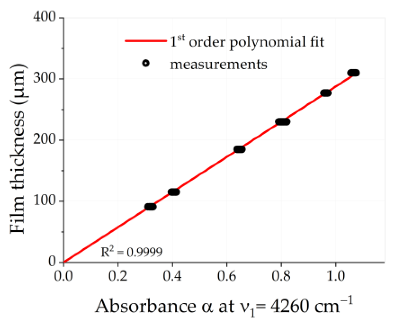
In the region above 4100 cm−1 and below 4400 cm−1 the spectra for common film thicknesses overlay become clearly visible, as shown in Figure 2a. This suggests that the absorbance spectra within this region are predominantly a function of , whereas the influences of and can be neglected. In turn, a linear dependency of the absorbance data to can be assumed such that a first-order polynomial is suited for calibration purposes. In Figure 3, values at the exemplary discrete wavenumber 4260 cm−1 are plotted in an --coordinate system. The corresponding linear fit is shown as a red line.
To assess the quality of the calibration, the root mean square error (RMSE) between the known and the calculated film thicknesses is introduced. Firstly, the fit coefficients and of the calibration polynomial are needed:
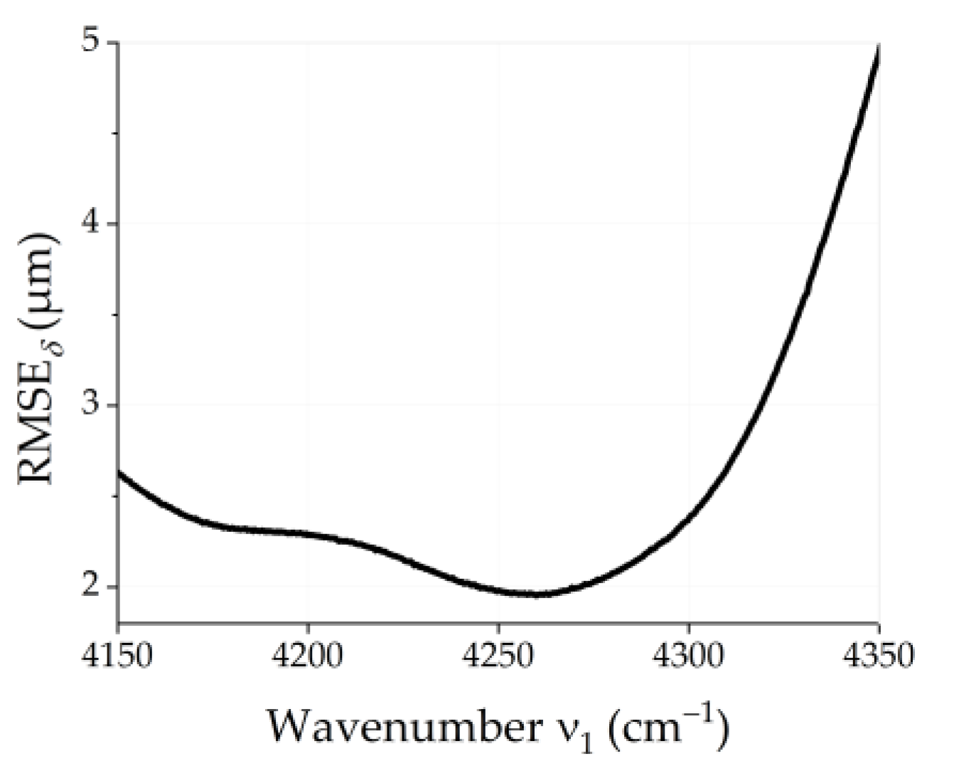
where a best fit is yielded in a least-squares sense. Secondly, is calculated by evaluating from the calibration set with known fit coefficients with Equation (3). The optimized wavelength for film thickness determination can then be assessed by calculating the s within the promising wavenumber region. The resulting curve over is shown in Figure 4. < 2 are achieved in the wavenumber region between 4245 cm−1 and 4271 cm−1.
3.2. Determination of the Additional Parameters of Temperature and Urea Concentration
In Figure 5, the same spectra are depicted as in Figure 2 but sorted by the film concentration. It becomes clear that no region can be identified where the curves of fixed concentration overlap; instead, they show interdependencies between the other film parameters. This can be explained by the fact that the film concentration and temperature are parameters that show a nonlinear dependency to (see Equation (2)), and, thus, a new calibration approach must be pursued.
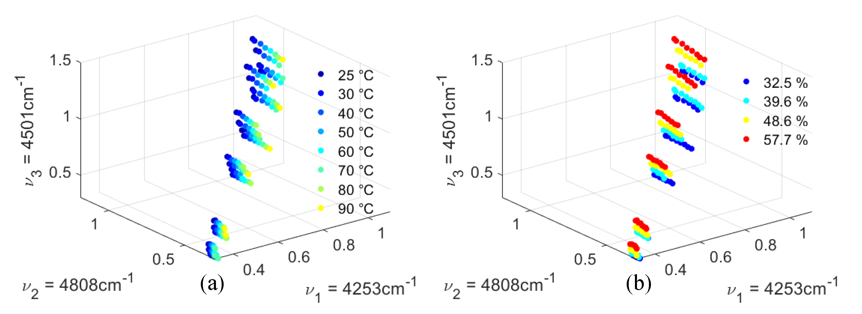
Firstly, the dependencies of the film parameters are visualized in the three-dimensional -- space. In Figure 6a, the scatter plot shows the absorbance data of the calibration data set at = 4253 cm−1, = 4808 cm−1 and = 4501 cm−1 with temperature-based color coding, while in Figure 6b, the same data are color coded with respect to the urea concentration. For both cases, a clear pattern can be identified, which suggests a dependency on the respective parameter to their location in the three-dimensional space. Since the visible tendencies point to a dependency of the parameter variation on the angles in the -- space, the data are transformed from Cartesian to spherical coordinates. In spherical coordinates, the data points are specified by the radial distance , the azimuthal angle and the elevation angle .
The resulting transformation is shown in the - space, while the radial distance is neglected, since this quantity is more closely connected to which was previously determined. The same transformed data set, depicted in Figure 7a, shows the data points with temperature-based color coding, while (b) is color coded with respect to the concentration. For each data set with same parameter value, a linear fit can be performed in the proposed - space, leading to a set of curves that approximately intersect on one common intersection point P. It becomes clear that the gradient of the fit curve is related to the sought-for parameter value. In terms of temperature, a higher positive gradient is proportional to higher temperature values (see Figure 7a), and higher concentration values correlate with higher negative gradients (see Figure 7b).
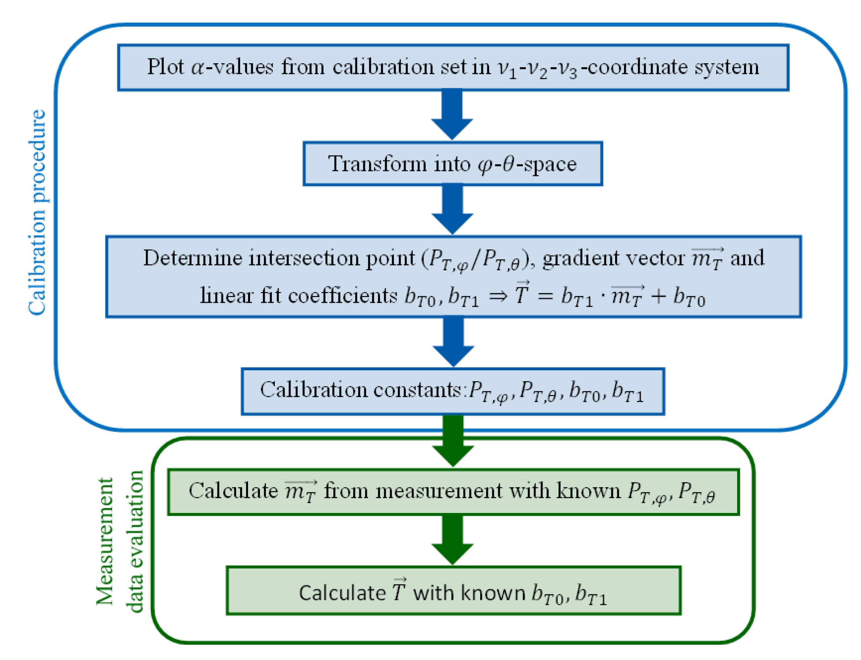
This observation suggests that a calibration can be performed by determining the coefficients of the linear fits of the set of curves and their respective intersection points and . With a known intersection point, the data from a subsequent measurement can be transformed to calculate the gradient and between the intersection point and and the measurement in the - space in the cases of the temperature and concentration, respectively. This way, the parameter of interest can be inferred from the resulting calibration curve, which is shown in Figure 8 (red solid line), where the predefined temperatures of the calibration data set are shown over the calculated gradients (Figure 8a) and mc (Figure 8b) as black dots. Similar to the film thickness calibration, the temperature and concentration calibration curves are gained by means of a linear least-squares first-order polynomial fit but in the - space. The resulting calibration curves for the temperature T and the concentration c can be described by
respectively.
The calibration, as well as the measurement of data and evaluation approach, is depicted as a schematic and summarized in Figure 9 for a better understanding. The calibration must be performed beforehand only once and the resulting fit coefficients, as well as intersection point coordinates, can be used for all subsequent measurements with the same wavenumber combination.
3.3. Optimization Procedures
The optimization conducted in order to identify the best wavenumber for film thickness determination is a straightforward process that can be performed by finding the minimum value of the curve, as shown in Figure 4. As described previously, the temperature and concentration determination rely on the data point locations in a suitable -- space. Only when combining the three appropriate wavenumbers -- will the transformation of the respective data points to the - space enable the calibration strategy shown in Section 3.2. Otherwise, no information about the unknown parameters can be gained. In this context, must be chosen to enable good film thickness results according to the procedure that is described in Section 3.1 and also to enable the reliable determination of the temperature and concentration.
Identifying the most suitable wavenumber combination is a far more complex task. This is due to the huge number of possible combinations, since more than 20.000 discrete wavenumbers have been sampled within the spectrum, leading to more than possible ---combinations. Therefore, it is not feasible to evaluate each possible combination. Additionally, within the proposed evaluation strategy, the coefficients for the set of linear fit curves, as well as the resulting common intersection point, must be optimized; this was carried out using a nonlinear least-squares solver in MATLAB (Version 2020b). This coefficient optimization must be performed for each wavenumber combination that is evaluated and assessed within the superordinate wavenumber optimization scheme.
The underlying problem that needs to be solved in the wavenumber optimization case is non-convex and of high dimensionality, which leads to the presence of several local minima as opposed to only one global minimum for convex problems. Thus, it is hardly possible to guarantee that the global minimum for the problem is found. The genetic algorithm implemented in MATLAB was used to solve this superordinate optimization problem since it is well suited to deal with problems where multiple local minima are present while avoiding being trapped within a local minimum.
Input parameters to the genetic algorithm solver are the complete absorbance spectra of the calibration set between approximately 3800 cm−1 to 13,000 cm−1, the corresponding wavenumber vector and the predefined film parameters of interest. Within the genetic algorithm solver (Figure 10, blue box), an initial wavenumber combination is randomly picked, and initial fit coefficients for the calibration are calculated. The latter are gained by independent fits of each curve for the same parameter data, while a first approximation of the intersection point can be calculated where the set of curves shows the smallest deviation. These initial fit coefficients and intersection point coordinates are then passed to the coefficient optimization loop (Figure 10, green box), where the final optimized values are calculated and returned to the genetic algorithm loop. Subsequently, the RMSE value is calculated, which acts as fitness function and assesses the quality of the calibration. Based on this, either a new combination of wavenumbers is chosen, and a new iteration is started, or the optimization of both the calibration coefficients as well as the wavenumber selection is finished.
The genetic algorithm optimization was performed a total of 70 times to create a pool of promising wavenumber combinations. This approach was necessary since each of the resulting wavenumbers must be checked for cross-absorptions with species that are likely to be present in the measurement domain, such as and . The best wavenumber combination, with respect to the calibration quality and exhibiting nearly no parasitic absorption, was found to be = 4253 cm−1, = 4808 cm−1 and = 4501 cm−1 as shown in Figure 6.
4. Results
To assess the results that are achievable with the proposed calibration procedures, a small test set was recorded, which consisted of seven measurements with c = 32.5%Mass, = 185 µm and temperatures ranging from room temperature (25 °C) to 70 °C.
4.1. Film Thickness Measurements
The film thickness was determined with the absorbance value extracted from the test measurement set at = 4253 cm−1. As described in Section 3.1, the calibration set was used to determine the linear fit curve. With and determined from the calibration and from the test set measurements, Equation (3) can be evaluated. The results of this evaluation are depicted in Figure 11, where the red circles show the ‘true’ film thickness, which is set by the spacer ring, and the calculated film thicknesses are represented by the black crosses. It is clearly visible that good results can be yielded with this calibration strategy. This is confirmed by the RMSE value, which amounts to 0.8 μm, while the maximum absolute error amounts to 1.3 μm.
In the experiment, the film thickness was determined with a micrometer screw at three positions on the spacer for which an uncertainty of roughly ±1 μm can be given. Additionally, dust particles or a small quantity of oil on the spacer surface can lead to a slight overestimation of the film thickness. Thus, an overall uncertainty for the film thickness of roughly 3 μm can be assumed.
4.2. Temperature and Concentration Measurements
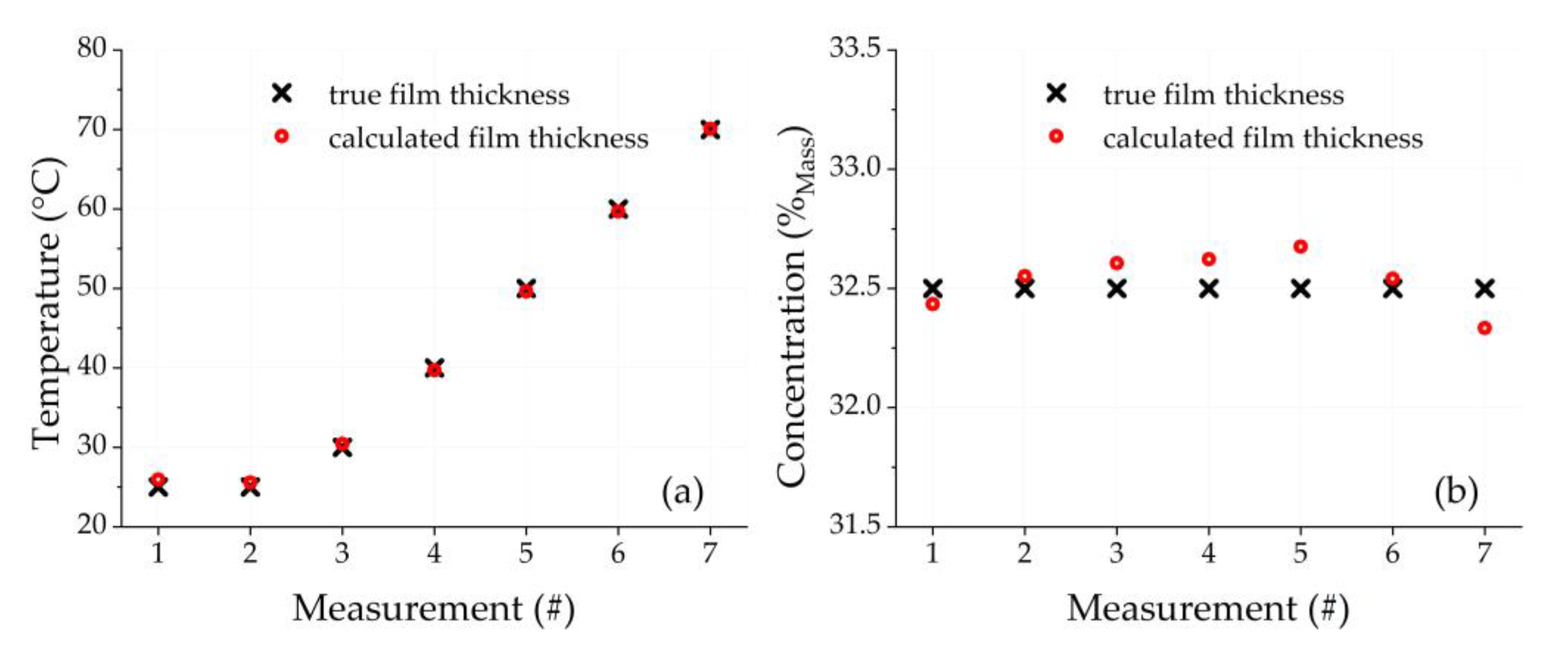
In the case of the temperature and concentration measurements, the absorbances of the test set are required at all three wavenumbers, = 4253 cm−1, = 4808 cm−1 and = 4501 cm−1. These values are extracted and subsequently transformed into the - space. Then, the respective gradients mT and mc are calculated based on the known intersection point coordinates PT for the temperature determination and Pc for the concentration. From the calibration performed beforehand with the calibration set, the linear fit coefficients are also known, and Equations (4a) and (4b) can be solved to gain the parameters of interest. Figure 12a shows the temperatures set in the calibration cell as red circles and the calculated values as black crosses, while Figure 12b depicts the true concentrations (red circles) and the respective evaluation results (black crosses). In both cases, good results can be achieved. The RMSE value for the temperature measurements amounts to 0.5 °C with a maximum absolute deviation of 1 °C. In terms of concentration, the RMSE value is 0.13%, and the maximum absolute deviation amounts to 0.18%.
The uncertainty of the type K thermocouple that was used in the experiment amounts to ±1.5 K, which can be increased by aging effects. With regard to the concentration of urea in water, the uncertainty of the mixing procedure that arises from the measurement of the liquid and solid components is within ±0.1%, while the uncertainty of the commercially available product is within ±0.7% such that an overall uncertainty can be estimated at well below ±1%.
5. Conclusions and Outlook
In this paper, we presented a novel evaluation approach to the laser-based determination of thin liquid Urea-Water film parameters of thickness, temperature and concentration. Firstly, a calibration set with known parameters was measured with an FTIR spectrometer. From the recorded transmission spectra, the absorbance spectra were calculated based on the three discrete wavenumbers that were selected for calibration purposes. For the film thickness determination, a straightforward and linear fit approach to the absorbance data at a single wavenumber showed excellent results. The parameters of temperature and concentration rely on the knowledge of the absorbances at all three selected wavenumbers. After the transformation of the data to spherical coordinates, the gradients between the data points and an intersection point that is known from the calibration can be calculated. This gradient then shows a linear dependency to the sought-for parameter. However, this approach is only feasible if , and are well selected, which is why optimization was carried out with a genetic algorithm. Finally, the results were checked to avoid cross-absorption with other relevant species.
The overall results that could be achieved were assessed with a test set. It was observed that the RMSE values for all film parameters were small, and, thus, the calibration approaches worked excellently. In the future, diode lasers operating at the selected wavelengths can be incorporated into a modular and compact sensor head to allow for non-intrusive in situ measurements with high temporal resolution.
Author Contributions
Experiment concept: S.v.d.K., G.G. and A.S.; data collection: G.G.; data evaluation and analysis: S.v.d.K.; writing—original draft preparation, S.v.d.K., V.E. and S.W.; algorithm: S.v.d.K.; data evaluation and discussion: S.v.d.K., V.E. and S.W.; writing—review and editing, S.v.d.K., S.W. and A.S.; supervision, S.W. All authors have read and agreed to the published version of the manuscript.
Funding
Funded by the Deutsche Forschungsgemeinschaft (DFG, German Research Foundation) Projektnummer 237267381-TRR 150.
Institutional Review Board Statement
Not applicable.
Informed Consent Statement
Not applicable.
Data Availability Statement
Data underlying the results presented in this paper are available at https://doi.org/10.48328/tudatalib-567 (accessed on 11 August 2021).
Conflicts of Interest
The authors declare no conflict of interest.
References
- May, R.K.; Evans, M.J.; Zhong, S.; Warr, I.; Gladden, L.F.; Shen, Y.; Zeitler, J.A. Terahertz in-line sensor for direct coating thickness measurement of individual tablets during film coating in real-time. J. Pharm. Sci. 2011, 100, 1535–1544. [Google Scholar] [CrossRef] [PubMed]
- Seong, J.; Kim, S.; Park, J.; Lee, D.; Shin, K.-H. Online noncontact thickness measurement of printed conductive silver patterns in Roll-to-Roll gravure printing. Int. J. Precis. Eng. Manuf. 2015, 16, 2265–2270. [Google Scholar] [CrossRef]
- Notay, R.S.; Priest, M.; Fox, M.F. The influence of lubricant degradation on measured piston ring film thickness in a fired gasoline reciprocating engine. Tribol. Int. 2019, 129, 112–123. [Google Scholar] [CrossRef] [Green Version]
- Cen, H.; Lugt, P.M. Film thickness in a grease lubricated ball bearing. Tribol. Int. 2019, 134, 26–35. [Google Scholar] [CrossRef]
- Drake, M.C.; Fansler, T.D.; Solomon, A.S.; Szekely, G.A. Piston Fuel Films as a Source of Smoke and Hydrocarbon Emissions from a Wall-Controlled Spark-Ignited Direct-Injection Engine. SAE Trans. 2003, 762–783. [Google Scholar] [CrossRef]
- Schulz, F.; Samenfink, W.; Schmidt, J.; Beyrau, F. Systematic LIF fuel wall film investigation. Fuel 2016, 172, 284–292. [Google Scholar] [CrossRef]
- Brack, W.; Heine, B.; Birkhold, F.; Kruse, M.; Deutschmann, O. Formation of Urea-Based Deposits in an Exhaust System: Numerical Predictions and Experimental Observations on a Hot Gas Test Bench. Emiss. Control Sci. Technol. 2016, 2, 115–123. [Google Scholar] [CrossRef]
- Grout, S.; Blaisot, J.-B.; Pajot, K.; Osbat, G. Experimental investigation on the injection of an Urea-Water solution in hot air stream for the SCR application. Evaporation and spray/wall interaction. Fuel 2013, 106, 166–177. [Google Scholar] [CrossRef]
- Schubring, D.; Shedd, T.A.; Hurlburt, E.T.; Schulz, F.; Schmidt, J.; Beyrau, F. Planar laser-induced fluorescence (PLIF) measurements of liquid film thickness in annular flow. Part II: Analysis and comparison to models Development of a sensitive experimental set-up for LIF fuel wall film measurements in a pressure vessel. Int. J. Multiph. Flow 2010, 36, 825–835. [Google Scholar] [CrossRef]
- Alonso, M.; Kay, P.J.; Bowen, P.J.; Gilchrist, R.; Sapsford, S. A laser induced fluorescence technique for quantifying transient liquid fuel films utilising total internal reflection. Exp. Fluids 2010, 48, 133–142. [Google Scholar] [CrossRef]
- Jia, Y.; Wu, T.; Dou, P.; Yu, M. Temperature compensation strategy for ultrasonic-based measurement of oil film thickness. Wear 2021, 476, 203640. [Google Scholar] [CrossRef]
- Reddyhoff, T.; Dwyer-Joyce, R.; Harper, P.; Sovány, T.; Nikowitz, K.; Regdon, G.; Kása, P.; Pintye-Hódi, K. Ultrasonic measurement of film thickness in mechanical seals//Raman spectroscopic investigation of film thickness. Seal. Technol. 2006, 28, 7–11. [Google Scholar] [CrossRef]
- Sovány, T.; Nikowitz, K.; Regdon, G.; Kása, P.; Pintye-Hódi, K. Raman spectroscopic investigation of film thickness. Polym. Test. 2009, 28, 770–772. [Google Scholar] [CrossRef] [Green Version]
- Bobbitt, J.M.; Mendivelso-Pérez, D.; Smith, E.A. Scanning angle Raman spectroscopy: A nondestructive method for simultaneously determining mixed polymer fractional composition and film thickness. Polymer 2016, 107, 82–88. [Google Scholar] [CrossRef] [Green Version]
- Pan, R. Near-Infrared Diode Laser Absorption Spectroscopy for Measuring Film Thickness, Temperature and Concentration in Liquid Films; Faculty of Engineering, Universität Duisburg-Essen: Duisburg, Germany, 2017. [Google Scholar]
- Schmidt, A.; Kühnreich, B.; Kittel, H.; Tropea, C.; Roisman, I.V.; Dreizler, A.; Wagner, S. Laser based measurement of water film thickness for the application in exhaust after-treatment processes. Int. J. Heat Fluid Flow 2018, 71, 288–294. [Google Scholar] [CrossRef]
- Schmidt, A.; Bonarens, M.; Roisman, I.V.; Nishad, K.; Sadiki, A.; Dreizler, A.; Hussong, J.; Wagner, S. Experimental Investigation of AdBlue Film Formation in a Generic SCR Test Bench and Numerical Analysis Using LES. Appl. Sci. 2021, 11, 6907. [Google Scholar] [CrossRef]
Figure 1.
Calibration cell: between the body (1) and the top plate (2), O-seals (3), wedged CaF2 windows (4) and a stainless steel spacer ring (5) are clamped to confine the thin liquid film within the spacer of a predefined height. The liquid temperature is set by heating cartridges (6) placed within the body [16].

Figure 2.
Absorbance spectra of all calibration measurements over the wavenumber. Spectra are color coded with respect to the film thickness and contain all T and c variations. (a) Enlarged section between 4100 cm−1 and 4450 cm−1.
Figure 2.
Absorbance spectra of all calibration measurements over the wavenumber. Spectra are color coded with respect to the film thickness and contain all T and c variations. (a) Enlarged section between 4100 cm−1 and 4450 cm−1.

Figure 3.
Known film thicknesses of the calibration set over respective absorbance values at 4260 cm−1 (black dots) and corresponding first-order polynomial fit of the data points (red line).
Figure 3.
Known film thicknesses of the calibration set over respective absorbance values at 4260 cm−1 (black dots) and corresponding first-order polynomial fit of the data points (red line).

Figure 4.
of the difference between the known and the calculated film thicknesses (calculated from the calibration set) over wavenumber .
Figure 4.
of the difference between the known and the calculated film thicknesses (calculated from the calibration set) over wavenumber .

Figure 5.
Absorbance spectra of all calibration measurements over the wavenumber. Spectra are color coded with respect to the film concentration of urea in water and contain all and variations.
Figure 5.
Absorbance spectra of all calibration measurements over the wavenumber. Spectra are color coded with respect to the film concentration of urea in water and contain all and variations.

Figure 6.
Three-dimensional scatter plot in -- space of absorbance data from the calibration set at the respective wavenumbers , and . (a) Dots are color coded with respect to film temperature. (b) Dots are color coded with respect to urea concentration.
Figure 6.
Three-dimensional scatter plot in -- space of absorbance data from the calibration set at the respective wavenumbers , and . (a) Dots are color coded with respect to film temperature. (b) Dots are color coded with respect to urea concentration.

Figure 7.
Two-dimensional scatter plot in - space of absorbance data from the calibration set transformed from -- space. Linear fit curves for the same parameter data are shown as black lines and the intersection point of fit curves P as a grey dot. (a) Dots are color coded with respect to film temperature. (b) Dots are color-coded with respect to urea concentration.

Figure 8.
(a) Predefined temperatures of each measurement over gradients calculated between measurements, intersection point in - space (black dots) and corresponding first-order polynomial fit (red solid line). (b) Predefined concentration values of each measurement over gradients mc are calculated between measurements, intersection point in - space (black crosses) and corresponding first-order polynomial fit (red solid line).

Figure 9.
Schematic of calibration procedure (blue box) and subsequent measurement data evaluation (green box) for temperature evaluation. Concentration evaluation is performed in the same manner.
Figure 9.
Schematic of calibration procedure (blue box) and subsequent measurement data evaluation (green box) for temperature evaluation. Concentration evaluation is performed in the same manner.

Figure 10.
Schematic of the wavenumber optimization procedure. For each wavenumber combination, the coefficient optimization (green box) must be performed within the superordinate wavenumber optimization by means of MATLAB’s genetic algorithm (blue box).
Figure 10.
Schematic of the wavenumber optimization procedure. For each wavenumber combination, the coefficient optimization (green box) must be performed within the superordinate wavenumber optimization by means of MATLAB’s genetic algorithm (blue box).

Figure 11.
Film thickness of test set. Red circles: true, predefined film thickness. Black crosses: calculated film thickness with calibration at = 4253 cm−1.
Figure 11.
Film thickness of test set. Red circles: true, predefined film thickness. Black crosses: calculated film thickness with calibration at = 4253 cm−1.

Figure 12.
Results for calibration performed at ν1 = 4253 cm−1, ν2 = 4808 cm−1 and ν3 = 4501 cm−1. (a) Red circles: true, predefined temperatures. Black crosses: calculated temperatures of test set. (b) Red circles: true, predefined concentrations. Black crosses: calculated concentrations of test set.


Table 1.
Parameter variations for calibration data set.
| Temperature T (°C) | ||
|---|---|---|
| 91 | 25 | 32.5 |
| 115 | 30 | 39.4 |
| 185 | 40 | 48.6 |
| 230 | 50 | 57.7 |
| 277 | 60 | |
| 310 | 70 | |
| 80 | ||
| 90 |
Publisher’s Note: MDPI stays neutral with regard to jurisdictional claims in published maps and institutional affiliations. |
© 2021 by the authors. Licensee MDPI, Basel, Switzerland. This article is an open access article distributed under the terms and conditions of the Creative Commons Attribution (CC BY) license (https://creativecommons.org/licenses/by/4.0/).
Share and Cite
MDPI and ACS Style
van der Kley, S.; Goet, G.; Schmidt, A.; Einspieler, V.; Wagner, S. Multiparameter Determination of Thin Liquid Urea-Water Films. Appl. Sci. 2021, 11, 8925. https://doi.org/10.3390/app11198925
AMA Style
van der Kley S, Goet G, Schmidt A, Einspieler V, Wagner S. Multiparameter Determination of Thin Liquid Urea-Water Films. Applied Sciences. 2021; 11(19):8925. https://doi.org/10.3390/app11198925
Chicago/Turabian Stylevan der Kley, Sani, Gabriele Goet, Anna Schmidt, Valentina Einspieler, and Steven Wagner. 2021. "Multiparameter Determination of Thin Liquid Urea-Water Films" Applied Sciences 11, no. 19: 8925. https://doi.org/10.3390/app11198925
Note that from the first issue of 2016, this journal uses article numbers instead of page numbers. See further details here.