Interoperability between Real and Virtual Environments Connected by a GAN for the Path-Planning Problem

Abstract

Path planning is a fundamental issue in robotic systems because it requires coordination between the environment and an agent. The path-planning generator is composed of two modules: perception and planning. The first module scans the environment to determine the location, detect obstacles, estimate objects in motion, and build the planner module’s restrictions. On the other hand, the second module controls the flight of the system. This process is computationally expensive and requires adequate performance to avoid accidents. For this reason, we propose a novel solution to improve conventional robotic systems’ functions, such as systems having a small-capacity battery, a restricted size, and a limited number of sensors, using fewer elements. A navigation dataset was generated through a virtual simulator and a generative adversarial network to connect the virtual and real environments under an end-to-end approach. Furthermore, three path generators were analyzed using deep-learning solutions: a deep convolutional neural network, hierarchical clustering, and an auto-encoder. Since the path generators share a characteristic vector, transfer learning approaches complex problems by using solutions with fewer features, minimizing the costs and optimizing the resources of conventional system architectures, thus improving the limitations with respect to the implementation in embedded devices. Finally, a visualizer applying augmented reality was used to display the path generated by the proposed system.

1. Introduction

In the past several decades, robotic systems have played an important role in artificial intelligence (AI), allowing solutions to existing problems that reduce the necessary resources. AI is the field of science that helps machines improve their functions, in the areas of logic, reasoning, planning, learning, and perception [1]. These features bring efficient performance to the systems in different fields.

One of the major topics in the AI field is the development of autonomous machines, such as robotic systems [2]. A robotic system is a reprogrammable multifunctional manipulator, designed to move materials, parts, tools, or specialized devices through various programmed movements to perform different tasks [3]. According to the classification of robotic systems, the autonomous level is the most advanced mode [4].

The field of robotic systems has seen great success in many problems by minimizing the resource requirements during online execution when moving between two points. Some of the contributions are surgical robotics [5], mobile robotics [6], hybrid locomotion [7], and bio-inspired robots [8,9]. According to the calculus of variations [10], a path is defined as the sum of the distances between two consecutive points defined by Equations (1) and (2). For this reason, a path is composed of a set of lines in space. Likewise, one of the principal features to describe a path is the level of safety with respect to avoiding obstacles. Therefore, path planning is the shortest distance between m obstacles O and the best value with the highest level of safety in a sequence of points p of length n. After adding a negative sign to the value, the maximum optimization safety problem is transformed into the minimum optimization problem, as defined in Equation (3) [11].

$$distance(p_i,p_{i+1})=\sqrt{{(x_i-x_{i+1})}^2+{(y_i-y_{i+1})}^2}$$

(1)

$$length\left(p\right)=\sum _{i=0}^{n}distance(p_i,p_{i+1})$$

(2)

$$safety\left(p\right)=-minmin\left\{minDistance(p_i{p}_{i+1},O_j)\right\}$$

(3)

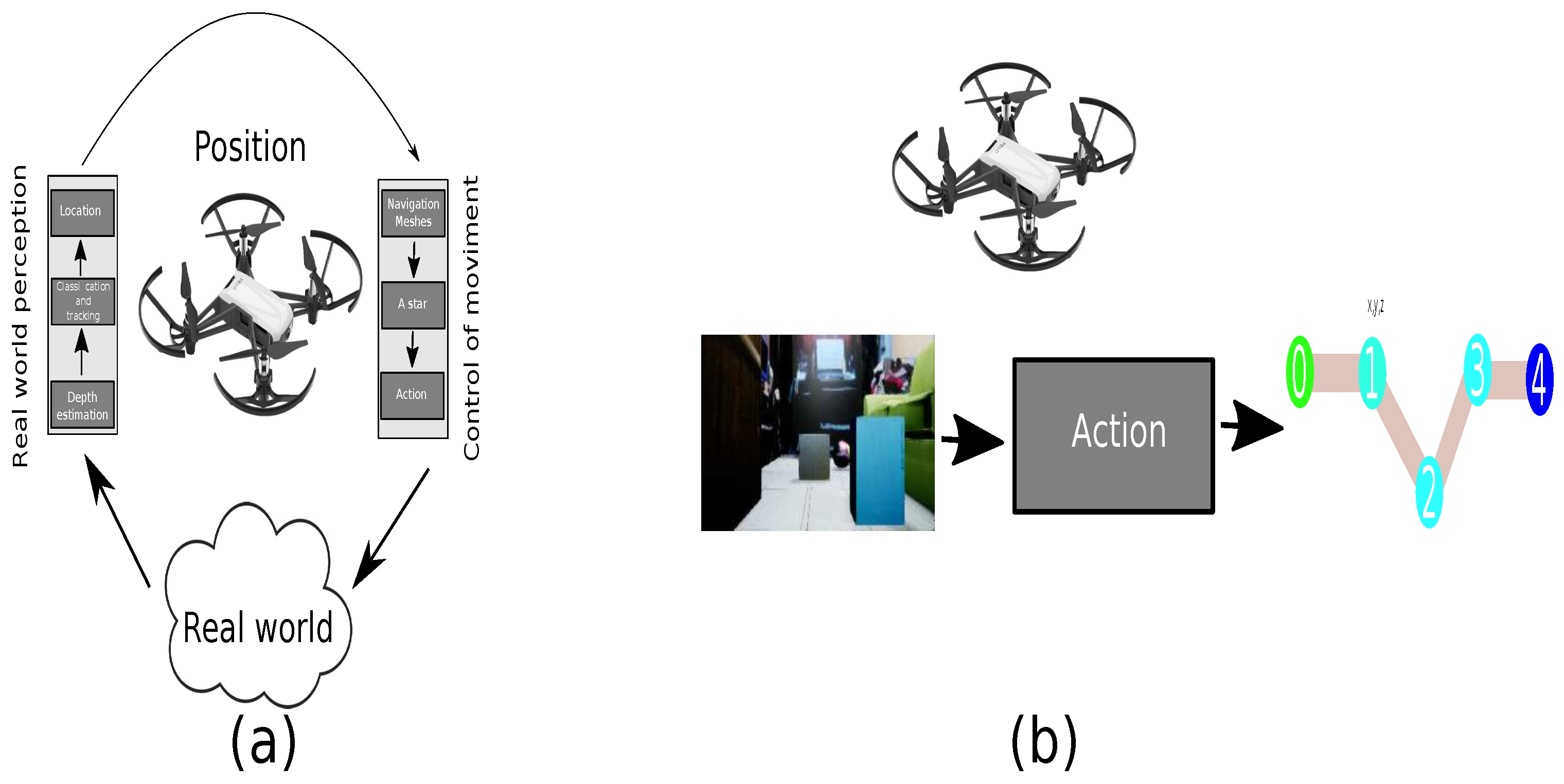
Consequently, the path-planning problem requires coordination between the environment and the agent. Hence, it is essential to define rules for the transition between states to achieve an objective. The path-planning problem mainly has two modules based on the definition of AI. The first is the planner, while the second module is the perception of the environment; this is shown in Figure 1 [12]. The problem is complex due to the robotic system’s characteristics, such as the battery, dimensions, and technologies to perceive the environment, including obstacles, illumination, and other agents in motion.

This architecture is efficient for robotic systems whose dimensions and battery are large, such as ground vehicles. In recent years, there has been a growing trend based on unmanned vehicle systems [13], for example micro aerial vehicles (MAVs), but these kinds of systems have reduced dimensions and a limited battery and are used in indoor environments. Subsequently, this architecture is unfeasible and inefficient. However, AI helps machines adopt new features to improve their limited performance.

Recent machine learning trends have addressed improving the weaknesses, such as some of the perception solutions with exciting applications in ground vehicles. Some contributions are the analysis of the road using RGB-D sensors [14], detecting and tracking to avoid collisions using RGB-D sensors [15], and extracting the features of the road map to generate trajectories through a LiDAR sensor [16], as well as developments in implementing different techniques to obtain external information [17]. Therefore, data have an essential role in the updated functionalities of the systems, which requires approaches to process the data, such as machine learning.

Machine-learning algorithms allow reducing the processing and resources needed, such as the end-to-end approach, allowing the collection of a dataset generated by physical sensors. This approach reduces the external factors [18], such as for specialized sensors, for example the fusion of LiDAR and camera sensors [19], a driving model for the steering control of autonomous vehicles [20], a controller for robot navigation using a deep neural network [21], and autonomous driving decisions based on the deep reinforcement learning approach [22]. The aims of these developments are the minimization of the resources needed and the improved performance of their respective architectures.

Likewise, one machine-learning solution is the generative adversarial network (GAN), composed of two kinds of networks, a generative and adversarial network. In this approach, both networks compete and generate new samples from a source of noise. Therefore, it is possible to relate a sample taken from one domain to another [23].

On the other hand, simulators, such as virtual reality, are capable of producing a model of reality. This technology consists of developing an immersive experience to explore a virtual world, which can bring us closer to the real world [24]. Subsequently, using an end-to-end approach, it is possible to reduce the computational time of the planner. Here, we propose three different solutions: a deep neural network [25], hierarchical clustering [26], and an auto-encoder [27], the aim of which is to map an input to a path generated by the conventional architecture.

Once the interoperability between the authentic and the virtual environment is achieved, it is possible to reduce the features of the current system through the transfer-learning approach [28] to implement it in embedded devices such as the Jetson nano and mobile devices.

As a consequence of the above, we made the following hypothesis. If a GAN allows connecting two domains, then it is possible to connect the real and virtual environments. Therefore, a dataset generated by a virtual simulator to estimate a path could be employed in an authentic environment, reducing the design time and costs. However, it is necessary to evaluate the performance of a problem that can be simulated and employed in the real world.

This paper makes the following contributions. First, the interoperability coefficient determines the number of samples of an authentic environment on a 2D plane. Second, the performance of the system on a virtual and an authentic environment results in different path-planning solutions. Additionally, we built a dataset based on a virtual environment, using an end-to-end approach. Finally, the proposal was evaluated on embedded devices.

The remainder of the manuscript is presented as follows. Section 2 reviews the background. The proposed work is described in Section 3. Likewise, the experiment and the analysis of the results are detailed in Section 4. Finally, conclusions and future work are presented in Section 5.

2. Related Works

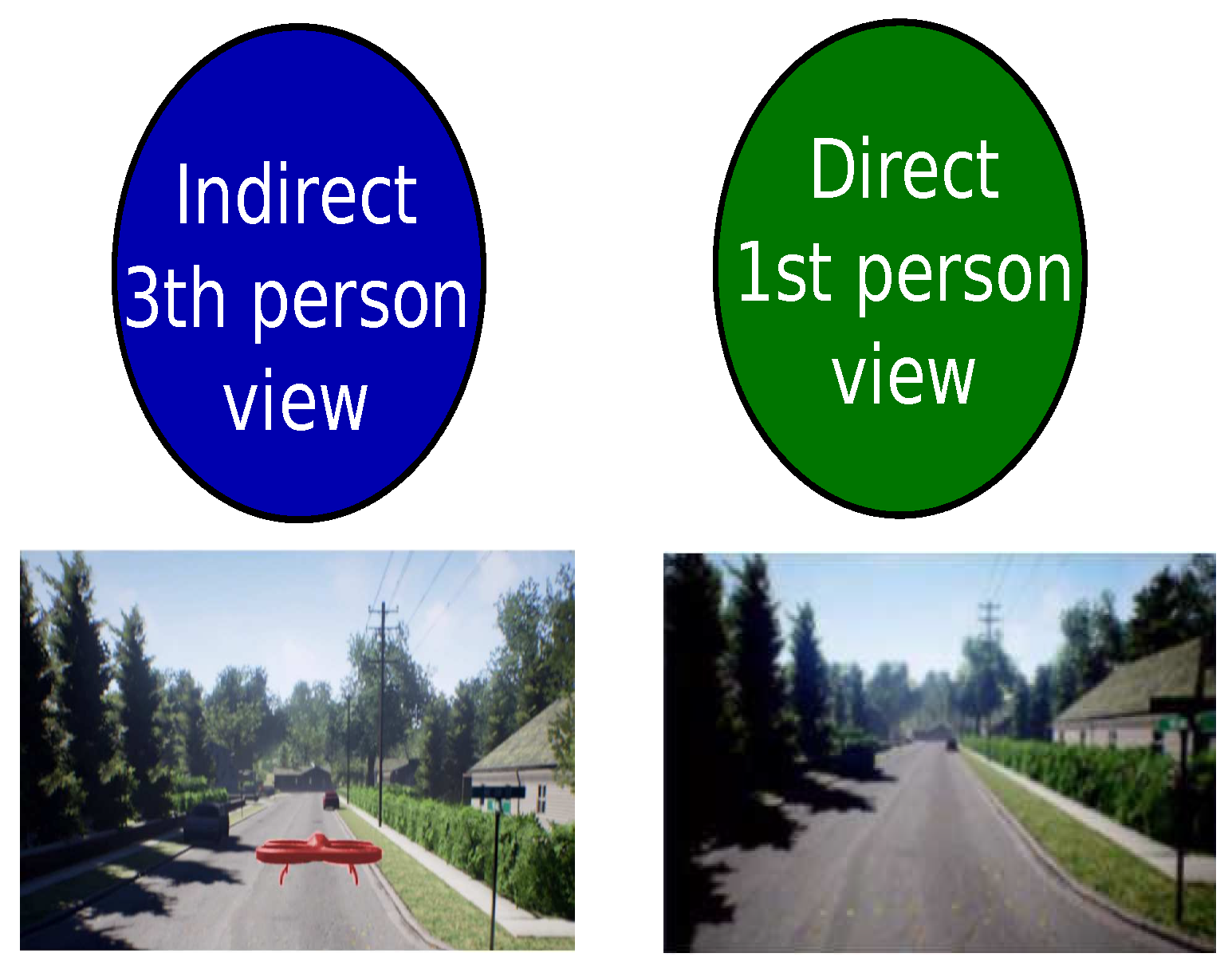
It is well known that robotic systems can move between two points, and the path-planning problem is composed of two principal modules based on the AI definition: perception and reasoning. Despite being two decoupled modules, both depend on each other. According to the direct and indirect state-of-the-art approaches, path-planning classification results in a direct and indirect point of reference for the robotic system in space, as shown in Figure 2.

The direct approach uses the robotic system as the point of reference to determine the movements. The kinematic movements of the robotic system describe the form of interacting with the environment. Various contributions have used a direct perspective approach, such as dynamic programming [29], soft robotics designing [30], and differential systems [31]. Secondly, the indirect perspective uses the environment as the principal element to capture the robotic system’s conditions. Thus, the sensing of the environment is a high priority, with relevant contributions using sampling-based algorithms [32], node-based algorithms [33], and bio-inspired algorithms [34].

Due to the features of MAVs, such as a flight time of approximately 15 min, small dimensions, and sensors such as a conventional camera and an IMU composed of two types of sensors of movement, a gyroscope and accelerometer, they present an optimization problem. Therefore, one of the main challenges in robotic systems is the optimization of the resources needed. For example, some works focused on generating solutions to optimize the flight time and navigation control to make the use of the systems’ resources more efficient [35,36,37].

This proposal implements an indirect approach using a virtual simulator because the analysis of the environment is of vital importance in executing an action. The virtual simulator has different elements to scan the environment, such as LiDAR, RGB-D, infrared sensors, ultrasonic sensors, radars, and 4D radars. The AirSim simulator [38] shows acceptable behavior to simulate a quadrotor. Moreover, this simulator allows the design of our 3D environment with different data inputs, such as the conventional input, the depth image, and the semantic image.

Secondly, a conventional algorithm for path planning was employed to associate a path for each sample generated by the virtual simulation. The $A^{*}$ algorithm finds short paths using graphs. A graph is a set of nodes with connections between them. Each node is a tuple indicating the destination node and the weight, which describes the connection. One particular characteristic of the algorithm is the movement, highlighting the diagonal between two points. The different movements are based on 45°, forming a star. The heuristics define the complexity of the $A^{*}$ algorithm, which executes in polynomial time with the implementation of the following expression in Equation (4) [39].

$$\left|h\left(x\right)-h^{\prime }\left(x\right)\right|=O\left(log\left(h^{\prime }\left(x\right)\right)\right)$$

(4)

Despite the $A^{*}$ algorithm’s advantages for path planning, it has inadequate performance when the nodes’ number increases. Therefore, we used a navigation mesh to reduce the number of nodes. A map in a virtual world is composed of triangles, and each triangle forms a primitive geometry. Thus, the centroid of each primitive geometry-shaped mesh is used, as shown in Figure [40].

AI represents the principles of the biological neuron, employing additive and multiplicative models composed of weights and biases. Simultaneously, an activation function completes the information flow step, generating a learning curve from an objective function. Therefore, it enables finding solutions to complex optimization problems by minimizing the cost of the objective function [41].

Deep learning is a technique that reduces the number of operations for considerable inputs with big dimensions, such as images [42]. The number of operations requires a large amount of processing and memory, causing these operations to be limited to small inputs. However, this approach aims to find characteristic vectors by the technique of reducing the data of the inputs that can be associated with the actions [43].

Although deep learning has been used in problems of classification [44,45] and regression [46,47], this approach has shown some limitations. Nevertheless, this fundamental approach to processing data for image analysis to generate images from a noise source has given rise to the GAN, which is based on the competition between two players [48]. The GAN is an architecture that uses two types of neural networks. The calculation of the entropy defines the cost functions of a GAN [49]. Therefore, the cost functions are defined as follows: the first network, called the generative network, is responsible for generating data from a noise source (Definition 1); the weights are adjusted after the evaluation of the second network, called the discriminator (Definition 2); the total cost function is the sum of both networks (Definition 3).

Definition 1.

Let n be the number of samples, $D_{1,2}$ be the cost function of the discriminator network, $G_{1,2}$ be the cost function of the generator network, and $Z_{1,2}$ be the noise source. The maximization of the cost function of the discriminator network is obtained according to the following expression:

$$M_{c{f}_{D_{1,2}}}=\frac{1}{n}·\sum _{i=0}^{n}log(D_{1,2}(i))+log(1-D_{1,2}(G_{1,2}(Z_{1,2}^i)))$$

(5)

Definition 2.

Let n be the number of samples, $D_{1,2}$ be the cost function of the discriminator network, $G_{1,2}$ be the cost function of the generator network, and $Z_{1,2}$ be the noise source. The minimization of the cost function of the generator network is obtained according to the following expression:

$$m_{c{f}_{G_{1,2}}}=\frac{1}{n}·\sum _{i=0}^n-log\left(D_{1,2}\left(G_{1,2}\left(Z^i\right)\right)\right)$$

(6)

Definition 3.

Let $D_{1,2}$ be the cost function of the discriminator network, $G_{1,2}$ be the cost function of the generator network, and $Z_{1,2}$ be the noise source. The full cost function of a simple GAN architecture is obtained according to the following expression:

$$GA{N}_{c{f}_{1,2}}=M_{c{f}_{D_{1,2}}}+m_{c{f}_{G_{1,2}}}$$

(7)

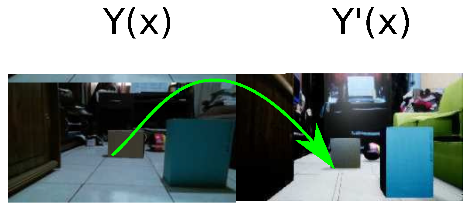
This approach provides the following solutions for the generation of images, obtaining incredible results: the transformation of an image to another representation of the data in a different domain [23]; generating data to create an image with different machine learning approaches [50]; generating sequences without pretraining data [51]; analyzing the convergence policies during the training [52]. In this proposal, two domains are required: are virtual and real. The GAN has a principal role in connecting both domains, as shown in Figure 3.

Finally, once the interoperability between two domains, the virtual and authentic environments, has been achieved, it is possible to implement the system on embedded devices by transfer learning, which is used to improve the learner from one domain by transferring information from another related domain [53]. In other words, the original system is changed by a new architecture that learns the same behavior, but in this case with fewer features.

Inspired by these contributions, the following procedure was defined to create a dataset in a virtual environment to reduce the development and implementation in low-cost systems. The following section describes the design of the dataset and each approach to generate a path based on the $A^{*}$ algorithm optimized with the navigation meshes.

3. Proposed Work

This section describes the methodology used to generate this proposal, which measures the performance of generating a path planning, whose analysis consists of creating a path plan by employing the end-to-end approach with virtual samples proven in an authentic environment. The approaches selected include a deep neural network, hierarchical clustering, and an auto-encoder to generate the path. These algorithms allow producing the path associated with each image.

Since exploration plays an essential role in unknown environments, the cost of implementing the physical requirements is expensive. Therefore, a virtual representation of the known authentic environment generates the samples for training. Once the virtual representation is built, it is possible to produce nonexistent conditions in the physical world and evaluate N iterations in a virtual environment without using the real world. However, the details of the environment are essential to associate a virtual representation with real samples.

One of the most significant challenges was the photorealism of the video game engine. Consequently, an analysis was performed to minimize this requirement by using low-quality images using Unreal Engine, which offers open-source images. Moreover, the framework developed by Microsoft, AirSim, allows simulations with a high degree of detail in the rendering [38].

3.1. Interoperability Coefficient to Connect the Virtual and Real Environments

We introduced the interoperability coefficient, which consists of determining a minimum number of real samples to connect the virtual and real domains using the GAN characteristics. This coefficient is composed of a correlation factor and the entropy generated by a GAN.

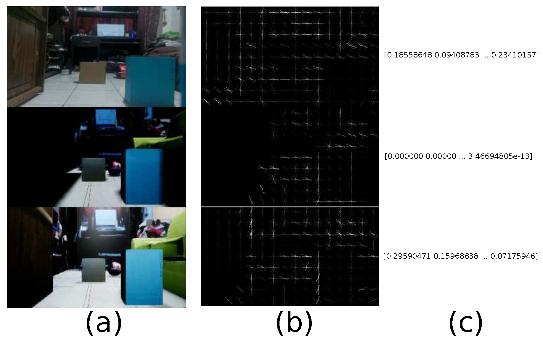
One of the tools to assess the correlation between two images is the HOG [54]. This algorithm allows measuring the comparison of the authentic environment and its virtual representation. This tool obtains a characteristic vector for each of the samples and offers a coefficient that indicates the similarity level, whose hyperparameters are: orientation equal to 8, pixels per cell equal to 32 × 32, and cells per block equal to 4 × 4. For example, Figure 4 shows a real sample and its virtual representation with two different detail levels. We observed that the first variation has essential lighting, and the second has a more significant number of directional lighting sources and materials that give more realism to the virtual environment.

Table 1. Correlation between real-world and virtual samples.

	Simple Environment Virtual vs. Real	Environment with Lights and Materials Virtual vs. Real
Factor Correlation      (mean)	0.3708	0.5490
Factor Correlation (std)	0.0824	0.0755

shows correlation measurements between 30 real-world samples and their virtual representation with two different detail levels. Since lights increase the detail level, the correlation coefficient of more detailed samples (lights and materials) is higher than essential light source samples. As the correlation coefficient between virtual samples created with video game engines and real examples is not high enough, the representation of the real world is inadequate.

Likewise, the other element that composes this coefficient is the joint entropy [49] by the virtual representation of the real image and the predicted fake image described in Equation (8).

Definition 4.

The interoperability coefficient is composed of the HOG determined by the detail of the virtual representation multiplied by the entropy of a virtual sample with its generated samples. Let $N_{real}$ be the number of real samples, $x_r$ the real image, and $x_v$ a virtual image to calculate the average HOG relation between both samples. Let $N_{GAN}$ be the number of samples gendered by the GAN, y the real sample’s virtual representation, $y^{\prime }$ a fake sample, $P{(}_{Y{Y}^{\prime }})$ the probability between a real and a fake sample, $H\left(y\right)$ the entropy of the real sample’s virtual representation, and $H\left(y^{\prime }\right)$ the fake sample’s entropy to determine the average joint entropy for each step and the sum of the entropy of both samples.

$$C_{interoperability}=\frac{{\sum }_k^{N_{real}}HOG(x_{r_k},x_{v_k})}{N_{real}}·\left(1-\frac{{\sum }_i^{N_{GAN}}\frac{-{\sum }_{y_i}{\sum }_{y_i^{\prime }}{P}_{Y_i{Y}_i^{\prime }}(y_i,y_i^{\prime })log{P}_{Y_i{Y}_i^{\prime }}\left(y_i{y}_i^{\prime }\right)}{H\left(y_i\right)+H\left(y_i^{\prime }\right)}}{N_{GAN}}\right)$$

(8)

Thus,

Table 2. Estimated minimum real samples needed to build the VR environment.

Number of Samples	Joint Entropy	Interoperability Coefficient
10	0.5894	0.1985
20	0.2567	0.2935
30	0.1564	0.4465
43	0.0957	0.5047

describes the interoperability coefficient to define the number of minimum samples used to build a virtual representation.

In this case, the HOG correlation is 0.5490, and the interoperability coefficient is 0.5047 in 43 real-world samples. For this reason, we recommend taking the number of samples when the interoperability coefficient is greater than 0.50. Hence, the details in the virtual representation are less than the authentic sample. It is essential to consider that the virtual representation must have enough information to allow deep learning [55] to use textures. Furthermore, the results showed that when the number of virtual representation samples increased their details in lights and materials, the interoperability coefficient must increase and the number of samples can be less. On the contrary, the joint entropy was low in the case that the dispersion was similar between the GAN architecture and virtual representation samples. However, this proposal’s restriction is the limited amount of real information, and the samples did not have enough details to avoid using more real samples.

3.2. Virtual Dataset

The $A^{*}$ algorithm is undoubtedly the most widely used because it has an approach that is implemented in the online execution and the level of implementation is low. In this way, this algorithm is only implemented to associate a path for each virtual sample. The $A^{*}$ algorithm is a graph-based trajectory optimization problem with a star-shaped motion evaluation (*). For each node, the algorithm finds the best path, obtaining a complexity of $O\left(n^2\right)$, and stores the nodes in memory, generating a problem with a large number of nodes. Likewise, Figure 5 shows a 3D scenario with the representation of spheres, which indicate the nodes to which the agent can move. The surface contains 91 nodes because we employed a DJI Tello drone whose minimum distance is 20 cm. Within the 91 nodes, 6 represent the spaces occupied by objects in motion in an instant of time.

The shortest path between an initial point and an endpoint in Figure 6 has 18 nodes. Due to the characteristics of the $A^{*}$ algorithm, it is necessary to perform the analysis of the occupied spaces, which makes it inefficient due to a more significant number of nodes. Therefore, the number of nodes is reduced.

The navigation mesh technique offers a reduction in the nodes required to find the best path. Figure 7 describes a manual representation of the scenario’s simplification using meshes where the nodes are grouped into an area to calculate the region’s centroid. Therefore, the number of nodes is reduced to four from an initial point to an endpoint using this technique. Another advantage of applying navigation meshes being able to move faster without jumping 20 cm each time, as shown in Figure 8.

The location of the objects follows the procedure in Figure 9. Although the simulator offers different input samples, a standard image was used as the input to create a location and classification network, as in Figure 9a. The subsequent detection of the objects in Figure 9b and segmentation of the depth images shown in Figure 9c results in a mask with the color of the objects moving on the known stage. Once the object is detected, the point cloud’s centroid is defined by a sphere, as shown in Figure 9d. Consequently, the state of the nodes covered by the sphere is occupied.

3.3. End-to-End Implementation

Robotic systems with the perception of 3D scenarios usually have many functions to estimate the locations of objects. Hence, usually, an efficient energy utilization and processing time are not very easy to achieve. Therefore, a knowledge database of the information was generated from the complex system to improve the efficiency.

Inspired by the end-to-end approach, the novel architecture integrates the module’s perception by depth estimation, a window predictor, and a tracker to estimate the objects’ locations. On the other hand, the planning module uses the $A^{*}$ algorithm with meshes. Therefore, implementing a knowledge database allows reducing the use of the subsystems of a complex system to a single block, as shown in Figure 10. In this way, the submodules are included in the optimized system.

In order to generate the dataset by an end-to-end approach, the following approaches were implemented: a deep convolutional neural network, hierarchical clustering, and an auto-encoder. Likewise, each approach has the following architecture defined in Figure 11 in common (the diagrams of the deep neural network were based on https://github.com/kennethleungty/Neural-Network-Architecture-Diagrams (28 October 2021)), because they share a characteristic vector.

3.3.1. Image to Path: Deep Convolutional Neuronal Network

The first approach implemented was using a deep convolutional neural network. The deep neural network is one of the best-known algorithms to extract features from an extensive dataset. This approach consists of using the deep convolutional network to extract the images whose outputs predict the number of the node to generate the path, as shown in Figure 12. Since it is a regression problem, the optimizer is the Adam optimizer with the following parameters: learning rate 0.001, $bet{a}_1$ 0.9, $bet{a}_2$ 0.999, epsilon 1 × 10⁻⁷, and the Mean-Squared Error (MSE) as a function to optimize Equation (9). In addition, each path is built of four points, where each couple of points represents the 2D position.

$$\frac{1}{n}·\sum _{i=1}^n{({\widehat{Y}}_i-Y_i)}^2$$

(9)

3.3.2. Image to Path: Hierarchical Clustering

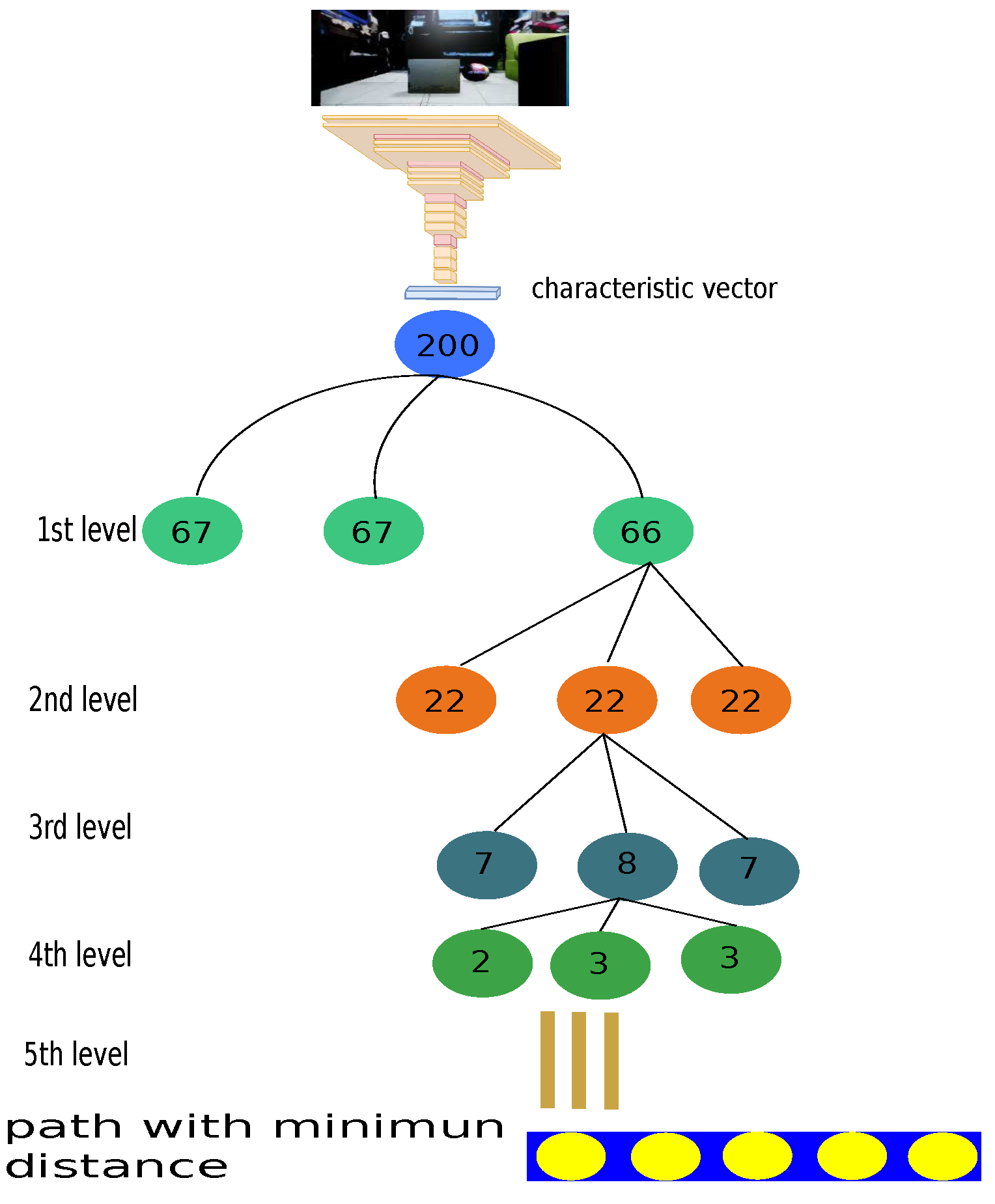
Another approach used in machine-learning algorithms is hierarchical clustering. A characteristic vector represents each image. The image has an associated path. This approach aims to split the data and find the characteristic vector with the minimum distance between two vectors. In this solution, a deep neural network was implemented to generate the characteristic vector. Hence, a feature vector was obtained for each sample, respectively having a path associated with it, shown in Figure 13. This model has five clustering levels where each color represents an updated cluster with the number of reduced elements until we obtain the vector with the minimum distance. Once this model is finished, instead of evaluating each sample (200), the number of evaluations is reduced to less than 15 by Equation (10) with number_of_levels equal to 5 and number_of_cluster to 3.

$$Operations<=(number\_of\_levels)\ast (number\_of\_cluster)$$

(10)

3.3.3. Image to Path: Auto-Encoder

There is evidence that recurring neural networks play a crucial role in the generated sequence of information, for example for natural language processing and situations requiring the implementation data sequences, for example time series analysis, where different types of recurring networks use auto-encoders [56]. The first is the encoder, which has deep, interconnected neuronal layers. The encoder function reduces the amount of information to create a characteristic vector that defines the dataset. Subsequently, the decoder processes the data [57], whose principal propose is to reconstruct the information from a characteristic vector. The decoder can reconstruct a characteristic vector into new associated information. A problem that uses this approach is the image caption problem, which generates a sequence of words to describe a photo [58].

The related works defined an encoder as a convolutional network that extracts the features from a set of samples. Consequently, this vector generates an input representing a sequence related to the image using recurring networks representing the decoder. A feature extraction network and an auto-encoder must generate the sequence of vectors representing the nodes to implement this architecture, as in Figure 14. Again, the optimizer is the Adam optimizer with the following parameters: learning rate 0.001, $bet{a}_1$ 0.9, $bet{a}_2$ 0.999, epsilon 1 × 10⁻⁷, and the cross-entropy error as a function to optimize Equation (11).

$$-\sum _i^C{t}_i·log\left(f{\left(s\right)}_i\right)$$

(11)

3.4. Strategy to Connect an Authentic Environment with Its Virtual Representation

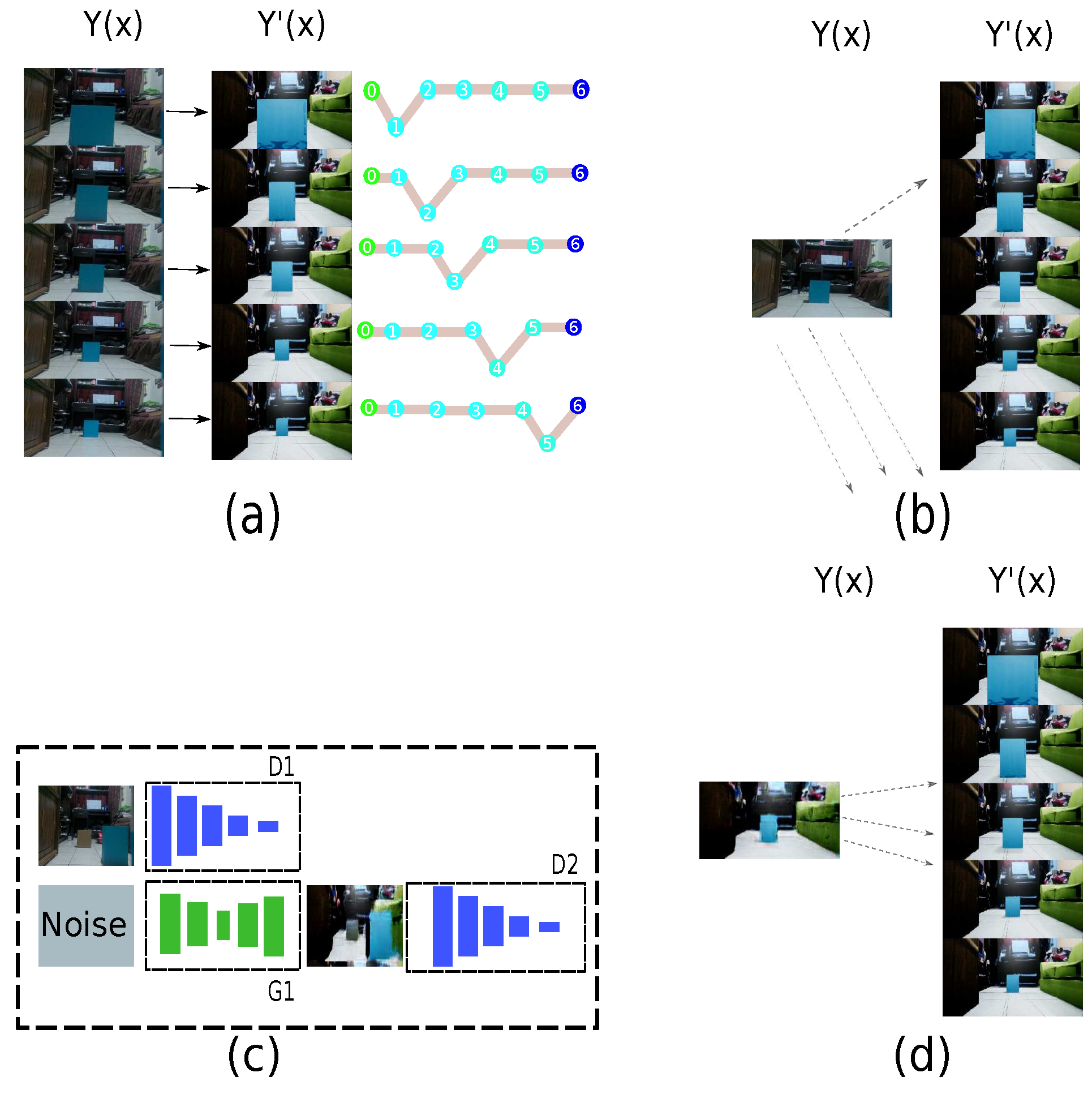
The following strategy is proposed to connect the virtual and real domain using the GAN, whose features are shown in Figure 15 and Figure 16 for generator and discriminator, respectively. The principal feature of this strategy is the connection between both domains, as shown in Figure 17a, where it is an authentic sample and its respective virtual representation with an associated path. This form of connecting both realities is adequate if the number of samples between both domains is the same. However, when an authentic image is not in the domain to predict the connection with the virtual image, the behavior is inadequate because the randomization is high in a one-to-one connection, as shown in Figure 17b. If the domain changes are implemented, the authentic image does not need to exist with the virtual domain. For this reason, the GAN employs the prediction of the virtual representation, having an approximation using the architecture in Figure 17c. Therefore, the randomness is reduced, as shown in Figure 17d, and the number of authentic samples is limited.

The domain changes from the real to the virtual environment are added to the module described in Figure 18, which is composed of the input (Figure 18a), the architecture with the GAN (Figure 18b), a deep convolutional network (Figure 18c), and the method to determine the output. Since each approach shares the characteristic vector, this proposal increases the system’s performance on embedded devices such as the Jetson nano 2G by Nvidia and the Android device, Moto X4. The updated parameters for embedded networks are shown in Figure 19.

Figure 20 summarizes the steps implemented in this development. As the first step, each virtual sample has an associated virtual path generated by the $A^{*}$ algorithm in the simulator, as shown in Figure 20a. Secondly, three deep-learning solutions are proposed to estimate a path, and the DCNN determines a characteristic vector that is common to them with virtual samples, as illustrated in Figure 20b. The third step describes the connection between both domains through a GAN. This network changes from the real domain to the virtual domain. Thus, the samples in the real domain are reduced to avoid a one-to-one connection, as shown in Figure 20c. Since the GAN requires considerable time, the transfer-learning approach is proposed to reduce this issue. The fourth step is to replace the GAN and characteristic vector called the domain changes with the transfer-learning approach. Therefore, a new model with fewer layers is trained to determinate the characteristic vector, but with fewer operations, as described the Figure 20d. However, it is necessary to consider that the domain change system estimated 50 samples to implement transfer learning. Finally, in the last step, instead of employing the GAN and characteristic vector as separate systems, both are included and placed as estimates of the virtual path with the three deep learning approaches from the real samples, as displayed in Figure 20e. In this way, the cost of the architecture is reduced, and its performance is improved.

4. Experimental Phase and Analysis

In order to evaluate the performance of the change of domain, a quantitative analysis was used. The following metrics were used to measure the depth estimation on generated images defined in the state-of-the-art [59]. Therefore, six indicators allow describing the performance:

• Average relative error (rel): $\frac{1}{n}{\sum }_p^n\frac{\left|Y_p-{\widehat{Y}}_p\right|}{Y_p}$;
• Root mean-squared error (rms): $\sqrt{\frac{1}{n}{\sum }_p^n{(Y_p-{\widehat{Y}}_p)}^2}$;
• Average ($lo{g}_{10}$) error: $\frac{1}{n}{\sum }_p^n\left|lo{g}_{10}(Y_p)-lo{g}_{10}({\widehat{Y}}_p)\right|$;
• Threshold accuracy (${\delta }_i$): % of $Y_p$ s.t. max($\frac{Y_p}{{\widehat{Y}}_p},\frac{{\widehat{Y}}_p}{Y_p}$) = $\delta <$thr for thr = $1.25,1.{25}^2,1.{25}^3$;

where $Y_p$ is a pixel in depth image Y, ${\widehat{Y}}_p$ is a pixel in estimated depth image $\widehat{Y}$, and n is the total number of pixels for each depth image.

Table 3. Performance of the quantitative metrics in our approach and the standard deviation of 50 samples. ↓, lower is better; ↑, higher is better.

Model	rel-std ↓	rms-std ↓	${log}_{10}$-std ↓	${\mathit{\delta }}_1$-std ↑	${\mathit{\delta }}_2$-std ↑	${\mathit{\delta }}_3$-std ↑
GAN	0.9481–0.5614	0.9418–0.2469	0.3479–0.0722	0.6767–0.0235	0.7925–0.0278	0.8491–0.0282
GAN-Noise	0.1693–0.2068	0.3862–0.1420	0.2392–0.0832	0.8538–0.0592	0.9334–0.0463	0.9624–0.0367

shows the performance of the domain change because an image taken in an authentic environment suggests the virtual representation of the respective authentic image. It is not necessary to obtain a value of zero in the result. Therefore, the metrics help describe the performance of the generated path with the different approaches.

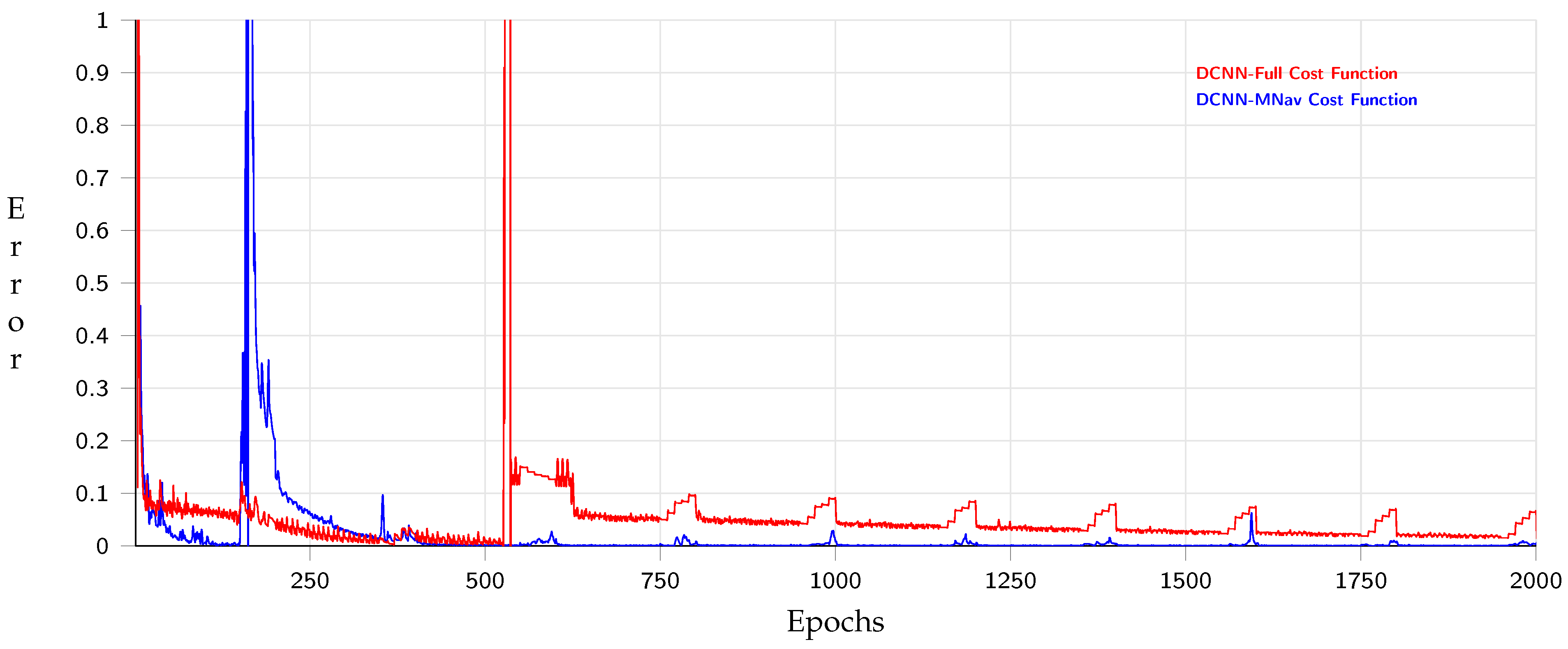
The performance of the Deep Convolutional Neural Network’s (DNCNN) training is shown in Figure 21, which shows the behavior on 1000 epochs with a normalized output, which had a precision of 90% with 20 test samples. The experiment consisted of describing the evaluation of two different experiments. The first contained all nodes generated by $A^{*}$ and the behavior throughout the navigation mesh (NavM), where the number of nodes was fewer than that of the full-path $A^{*}$.

Figure 22 represents the behavior of the auto-encoder (AED) training, where 5000 epochs had a precision of 95% with 20 test samples. This experiment, similar to the evaluation before, showed two behaviors with all nodes created by $A^{*}$ and with the navigation mesh reducing the number of nodes in the path.

In this case, hierarchical clustering was not used because this approach did not require training. According to the results, the behaviors of the deep convolutional neural network and auto-encoder with navigation mesh converged before as the output contained fewer nodes than the full path. On the other hand,

Table 4. Performance of the end-to-end approach and its standard deviation in 50 samples. ↓, lower is better; ↑, higher is better.

Model	Accuracy Euclidean Distance (mean-std) ↓	Accuracy Manhattan Distance (mean-std) ↓	Accuracy Cosine Similarity (mean-std) ↓	Coefficient Free Collision ↑
DCNN-one2one	53.8667 ± 3.9055	128.8 ± 14.5931	0.7069 ± 0.0586	0.02
DCNN-Full	22.6847 ± 3.5832	86.7401 ± 6.5722	0.8996 ± 0.03491	0.66
DCNN-MNav	8.4568 ± 1.5475	22.1415 ± 4.2568	0.91454 ± 0.0355	0.84
HC-one2one	15.1254 ± 2.4585	32.1346 ± 3.1354	0.8745 ± 0.02499	0.82
HC-Full	10.1411 ± 4.2164	24.2668 ± 3.1465	0.9224 ± 0.02587	0.92
HC-MNav	4.2145 ± 1.2441	9.2154 ± 1.8795	0.9952 ± 0.001256	0.96
AED-one2one	41.6589 ± 2.6425	130.0512 ± 2.9717	0.7496 ± 0.2654	0.04
AED-Full	19.6318 ± 2.1653	49.7123 ± 9.5722	0.9496 ± 0.0211	0.82
AED-MNav	4.7855 ± 2.1412	7.6569 ± 3.1336	0.98924 ± 0.01989	0.92

describes the behavior of the evaluation of the vectors based on the Euclidean distance (Equation (12)), the Manhattan distance (Equation (13)), and the similarity by the cosine (Equation (14)) used to analyze the difference between the expected vector x and the generated vector y. The free collision coefficient of Equation (15) determines if at least one node generates an inadequate path quantitatively.

$$euclidean=\sqrt{\sum _{i=0}^k{(\overrightarrow{x_i}-\overrightarrow{y_i})}^2}$$

(12)

$$manhattan=\sum _{i=0}^k\left|(\overrightarrow{x_i}-\overrightarrow{y_i})\right|$$

(13)

$$cosinesimilarity=\frac{\overrightarrow{x}·\overrightarrow{y}}{∥\overrightarrow{x}∥∥\overrightarrow{y}∥}$$

(14)

$$C_{freecollision}=1-\frac{{\sum }_{i=1}^{N_{samples}}\left\{\begin{array}{c}ifexistscollisionc=1\\ elsec=0\end{array}\right.}{N_{samples}}$$

(15)

The three models with one-to-one linking had high randomization. Therefore, it was essential to connect both realities with the GAN to reduce that random behavior. In this experiment, each node was composed of two points of the output. For example, if the output vector had ten values, this means that the path had five nodes. The results show that the solution with the navigation mesh improved the performance because the number of nodes was fewer than the full path.

Besides, the model with the best behavior was the hierarchical clustering because this model is associated with the sample existing in the training samples, but samples in the dataset generate the path. Therefore, this approach was the best with respect to the free collision coefficient. However, all possible solutions must appear in the dataset to improve the accuracy compared with the auto-encoder. On the contrary, the deep convolutional neural network had a competitive behavior, but the error increased, while the path was long. Finally, the auto-encoder model predicted the sequence; hence, this approach reduced the number of training samples more than hierarchical clustering.

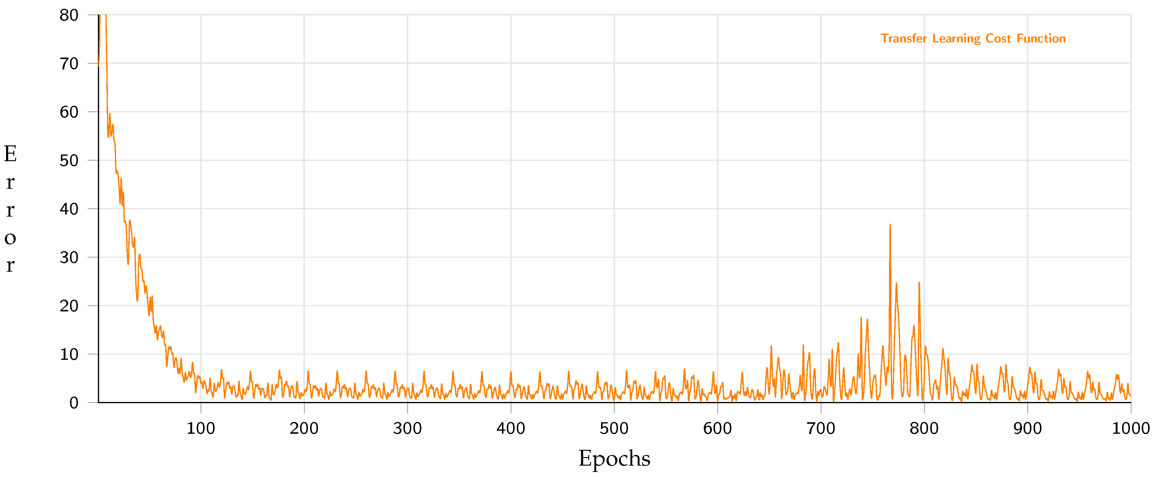
Concerning the execution on embedded devices through a model with fewer operations, Figure 23 shows that the performance of 1000 epochs for the optimized network for mobile devices using a transfer-learning approach had a precision of 95% with 20 test samples.

In order to validate the accuracy, the evaluation of the metrics was repeated, including two models with different floats generated by Tensorflow-lite because the GPU’s performance increases with a short float size.

Table 5. Performance of the transfer-learning approach and its standard deviation in 50 samples. ↓, lower is better; ↑, higher is better.

Model	Size of Word	Accuracy Euclidean Distance (mean-std) ↓	Accuracy Manhattan Distance (mean-std) ↓	Accuracy Cosine Similarity (mean-std) ↓	Coefficient      Free Collision ↑
DCNN-Full	Float16	27.9917 ± 2.1647	107.1066 ± 7.3813	0.9358 ± 0.2028	0.68
	Float32	27.9910 ± 2.1641	107.1053 ± 7.3780	0.9358 ± 0.2028	0.72
DCNN-MNav	Float16	10.1415 ± 1.5896	28.7415 ± 2.4785	0.9748 ± 0.01811	0.76
	Float32	10.1413 ± 1.5892	28.7408 ± 2.4779	0.9749 ± 0.01814	0.78
HC-Full	Float16	12.6325 ± 1.6896	19.1415 ± 3.1415	0.9813 ± 0.01258	0.92
	Float32	12.6319 ± 1.6888	19.1410 ± 3.1404	0.9814 ± 0.01256	0.92
HC-MNav	Float16	5.21227 ± 1.9859	10.0046 ± 1.0156	0.9916 ± 0.0009	0.94
	Float32	5.21223 ± 1.9853	10.0038 ± 1.0149	0.9916 ± 0.0011	0.94
AED-Full	Float16	17.1215 ± 2.4475	38.8528 ± 2.2332	0.9415 ± 0.0154	0.82
	Float32	17.1208 ± 2.4470	38.8520 ± 2.2325	0.9416 ± 0.0152	0.84
AED-MNav	Float16	4.7485 ± 0.9869	7.4415 ± 1.2023	0.9814 ± 0.0224	0.88
	Float32	4.7478 ± 0.9862	7.4409 ± 1.2018	0.9814 ± 0.0224	0.88

describes the performance of the test evaluation vectors on different models with full nodes and the navigation mesh with both sizes of float points in 16 bit and 32 bit, respectively.

The main difference between the two types of word size is the free path coefficient because the Float16 word size differs slightly by one node. This behavior was due to a decrease in the word size precision in the operations. However, the model that affected this behavior the most was the DCNN-Full model since it has morenodes, and the weights change their behavior due to the word size differences. Another factor that affects its behavior is that the normalized output is multiplied by a constant, which caused the error to increase.

Likewise, the AED model maintained a similar behavior in its two variants, not affecting the word size. In this way, this approach is the most suitable solution for path generation compared to scenarios involving more nodes. Finally, the HC model had an acceptable behavior, but this model requires an increase in the number of samples in the training set to cover more possibilities and increases the development time.

Table 6. Frames per second on embedded devices.

Device	Float16 (FPS)	Flotat32 (FPS)
Jetson nano 2G Tensorflow-lite	11	10
Jetson nano 2G Tensor RT	41	10
Android device Moto X4 CPU-4 threads	14	12
Android device Moto X4 GPU	20	16
Android device Moto X4 NN-API	6	6

describes the performance when implemented on embedded devices, such as the Jetson nano 2G and the Android device, Moto X4, with a 630 GPU and a CPU with 2GHz. The Jetson nano 2G can execute the model using the specific Nvidia technology, RTTensor, and only the CPU. Similarly, the Android device can also execute the model using a CPU, a GPU, and the API developed by Google called NN-API.

According to [60], when a system achieves at least 10 FPS, it is considered a real-time system. Thus, the evaluation showed that the performance took advantage of the Nvidia technology, as the RTTensors, with Float16. Further, the Android device also executed on the GPU and the reduced size of the floating point. Unfortunately, the NN-API gave an inadequate performance since this Android device is limited compared to high-performance Android devices. The models presented in this paper can be improved by increasing the number of layers or decreasing the number of nodes and implementing strategies that enhance the behavior for each approach.

Figure 24 shows the path generated by this proposal. We implemented an augmented reality system on a mobile device to illustrate the path. In this Figure 24a,b, a successful path plan is shown, and a node represents each step. Each node has a label to indicate what is the next step. The path has all the nodes from the star to the final point. The path changes the form of the objects in the environment.

In summary, this proposal provided acceptable behavior. However, one of the main characteristics of machine learning is that there is no generalized solution. As described in the experiment, there are different solutions, but each has its advantages and disadvantages. The decision depends on the problem and the designer. Furthermore, it is essential to mention that external conditions, such as lighting and shadows generated in the scenario, affected the performance. The samples with a high error value were generated by the ambient lighting and the shadows generated by the objects. When the lighting was constant and the shadows were eliminated with spotlighting, these unexpected effects decreased. Therefore, adding more samples with a variety of illumination and shading in the virtual dataset should be considered.

5. Conclusions and Future Work

The main characteristic of GANs is the connection between two or more domains. However, the potential of these networks has not been studied in depth. Therefore, this proposal introduced a novel perspective for developing systems based on the interoperability between real and virtual environments to generate a path for a MAV. In this way, virtual environments have an essential role in generating the dataset employed in real scenarios with limited characteristics. Likewise, three models based on deep learning approaches were implemented and analyzed. Although the path estimate was based on the connection with a virtual representation, each model demonstrated successful performance. However, it is complicated to define an ideal model because each model can be improved from a particular solution to reduce the number of collisions.

This method has advantages and disadvantages: the advantages are the reduction of the development times, fewer specialized sensors, and a limited number of samples of an authentic scenario based on the proposed interoperability coefficient; the disadvantages are the external factors that are difficult to control in the real world, such as illumination and shadows. Finally, the answer to the hypothesis is that techniques to change a domain into environments allow connecting the real with the virtual environment under ideal conditions such as controlled illumination and known scenarios. As future work, it is required to employ algorithms to generate 3D paths and implement them in a real MAV. Furthermore, the coefficient to determine how many real-world samples must be improved to obtain an optimal connection between both realities.

References

- Lighthill, I. Artificial Intelligence: A General Survey; Artificial Intelligence: A Paper Symposium; Science Research Council: London, UK, 1973. [Google Scholar]
- Althoefer, I.K.; Konstantinova, J.; Zhang, K. (Eds.) Towards Autonomous Robotic Systems; Lecture Notes in Computer Science; Springer: Berlin/Heidelberg, Germany, 2019. [Google Scholar] [CrossRef]
- Tian, Y.; Chen, X.; Xiong, H.; Li, H.; Dai, L.; Chen, J.; Xing, J.; Chen, J.; Wu, X.; Hu, W.; et al. Towards human-like and transhuman perception in AI 2.0: A review. Front. Inf. Technol. Electron. Eng. 2017, 18, 58–67. [Google Scholar] [CrossRef]
- Alenazi, M.; Niu, N.; Wang, W.; Gupta, A. Traceability for Automated Production Systems: A Position Paper. In Proceedings of the 2017 IEEE 25th International Requirements Engineering Conference Workshops (REW), Lisbon, Portugal, 4–8 September 2017; pp. 51–55. [Google Scholar]
- Su, Y.-H.; Munawar, A.; Deguet, A.; Lewis, A.; Lindgren, K.; Li, Y.; Taylor, R.H.; Fischer, G.S.; Hannaford, B.; Kazanzides, P. Collaborative Robotics Toolkit (CRTK): Open Software Framework for Surgical Robotics Research. In Proceedings of the 2020 Fourth IEEE International Conference on Robotic Computing (IRC), Taichung, Taiwan, 9–11 November 2020; pp. 48–55. [Google Scholar] [CrossRef]
- Santos, J.; Gilmore, A.N.; Hempel, M.; Sharif, H. Behavior-based robotics programming for a mobile robotics ECE course using the CEENBoT mobile robotics platform. In Proceedings of the 2017 IEEE International Conference on Electro Information Technology (EIT), Lincoln, NE, USA, 14–17 May 2017; pp. 581–586. [Google Scholar] [CrossRef]
- Marko, B.; Prajish, S.; Dario, B.; Heike, V.; Marco, H. Rolling in the Deep–Hybrid Locomotion for Wheeled-Legged Robots Using Online Trajectory Optimization. IEEE Robot. Autom. Lett. 2020, 5, 3626–3633. [Google Scholar] [CrossRef] [Green Version]
- Luneckas, M.; Luneckas, T.; Kriaučiūnas, J.; Udris, D.; Plonis, D.; Damaševičius, R.; Maskeliūnas, R. Hexapod Robot Gait Switching for Energy Consumption and Cost of Transport Management Using Heuristic Algorithms. Appl. Sci. 2021, 11, 1339. [Google Scholar] [CrossRef]
- Luneckas, M.; Luneckas, T.; Udris, D.; Plonis, D.; Maskeliunas, R.; Damasevicius, R. A hybrid tactile sensor-based obstacle overcoming method for hexapod walking robots. Intell. Serv. Robot. 2021, 14, 9–24. [Google Scholar] [CrossRef]
- Zabarankin, M.; Uryasev, S.; Murphey, R. Aircraft routing under the risk of detection. Nav. Res. Logist. 2006, 53, 728–747. [Google Scholar] [CrossRef]
- Xue, Y.; Sun, J.-Q. Solving the Path Planning Problem in Mobile Robotics with the Multi-Objective Evolutionary Algorithm. Appl. Sci. 2018, 8, 1425. [Google Scholar] [CrossRef] [Green Version]
- Schwartz, J.T.; Sharir, M. On the piano movers’ problem: II. General techniques for computing topological properties of real algebraic manifolds. Adv. Appl. Math. 1983, 4, 298351. [Google Scholar] [CrossRef] [Green Version]
- Chabot, D. Trends in drone research and applications as the Journal of Unmanned Vehicle Systems turns five. J. Unmanned Veh. Syst. 2018, 6, vi–xv. [Google Scholar] [CrossRef] [Green Version]
- Tanaka, M. Robust parameter estimation of road condition by Kinect sensor. In Proceedings of the SICE Annual Conference (SICE), Akita, Japan, 18–19 August 2012; pp. 197–202. [Google Scholar]
- Yue, H.; Chen, W.; Wu, X.; Zhang, J. Kinect based real time obstacle detection for legged robots in complex environments. In Proceedings of the 2013 IEEE 8th Conference on Industrial Electronics and Applications (ICIEA), Melbourne, VIC, Australia, 19–21 June 2013; pp. 205–210. [Google Scholar] [CrossRef]
- Chen, J.; Tian, S.; Xu, H.; Yue, R.; Sun, Y.; Cui, Y. Architecture of Vehicle Trajectories Extraction With Roadside LiDAR Serving Connected Vehicles. IEEE Access 2019, 7, 100406–100415. [Google Scholar] [CrossRef]
- Kristian, K.; Edouard, I.; Hrvoje, G. Computer Vision Systems in Road Vehicles: A Review. arXiv 2013, arXiv:1310.0315. [Google Scholar]
- Wang, T.; Wu, D.J.; Coates, A.; Ng, A.Y. End-to-end text recognition with convolutional neural networks. In Proceedings of the 21st International Conference on Pattern Recognition (ICPR2012), Tsukuba, Japan, 11–15 November 2012; pp. 3304–3308. [Google Scholar]
- Warakagoda, N.; Dirdal, J.; Faxvaag, E. Fusion of LiDAR and Camera Images in End-to-end Deep Learning for Steering an Off-road Unmanned Ground Vehicle. In Proceedings of the 2019 22th International Conference on Information Fusion (FUSION), Ottawa, ON, Canada, 2–5 July 2019; pp. 1–8. [Google Scholar]
- Wu, T.; Luo, A.; Huang, R.; Cheng, H.; Zhao, Y. End-to-End Driving Model for Steering Control of Autonomous Vehicles with Future Spatiotemporal Features. In Proceedings of the 2019 IEEE/RSJ International Conference on Intelligent Robots and Systems (IROS), Macau, China, 3–8 November 2019; pp. 950–955. [Google Scholar] [CrossRef]
- Wang, J.K.; Ding, X.Q.; Xia, H.; Wang, Y.; Tang, L.; Xiong, R. A LiDAR based end to end controller for robot navigation using deep neural network. In Proceedings of the 2017 IEEE International Conference on Unmanned Systems (ICUS), Beijing, China, 27–29 October 2017; pp. 614–619. [Google Scholar] [CrossRef]
- Huang, Z.; Zhang, J.; Tian, R.; Zhang, Y. End-to-End Autonomous Driving Decision Based on Deep Reinforcement Learning. In Proceedings of the 2019 5th International Conference on Control, Automation and Robotics (ICCAR), Beijing, China, 19–22 April 2019; pp. 658–662. [Google Scholar] [CrossRef]
- Zhu, J.; Park, T.; Isola, P.; Efros, A.A. Unpaired Image-to-Image Translation Using Cycle-Consistent Adversarial Networks. In Proceedings of the 2017 IEEE International Conference on Computer Vision (ICCV), Venice, Italy, 22–29 October 2017; pp. 2242–2251. [Google Scholar] [CrossRef] [Green Version]
- Jung, T.; Dieck, M.C.T.; Rauschnabel, P.A. (Eds.) Augmented Reality and Virtual Reality. In Progress in IS; Springer: Berlin/Heidelberg, Germany, 2020. [Google Scholar] [CrossRef]
- Huang, J.Y.; Hughes, N.J.; Goodhill, G.J. Segmenting Neuronal Growth Cones Using Deep Convolutional Neural Networks. In Proceedings of the 2016 International Conference on Digital Image Computing: Techniques and Applications (DICTA), Gold Coast, Australia, 30 November–2 December 2016; pp. 1–7. [Google Scholar] [CrossRef]
- Wenchao, L.; Yong, Z.; Shixiong, X. A Novel Clustering Algorithm Based on Hierarchical and K-means Clustering. In Proceedings of the 2007 Chinese Control Conference, Wuhan, China, 26–31 July 2007; pp. 605–609. [Google Scholar] [CrossRef]
- Cui, Q.; Pu, P.; Chen, L.; Zhao, W.; Liu, Y. Deep Convolutional Encoder-Decoder Architecture for Neuronal Structure Segmentation. In Proceedings of the 2018 International Conference on Control, Artificial Intelligence, Robotics & Optimization (ICCAIRO), Prague, Czech Republic, 19–21 May 2018; pp. 242–247. [Google Scholar] [CrossRef]
- Shao, L.; Zhu, F.; Li, X. Transfer Learning for Visual Categorization: A Survey. IEEE Trans. Neural Networks Learn. Syst. 2015, 26, 1019–1034. [Google Scholar] [CrossRef]
- Si, J.; Yang, L.; Lu, C.; Sun, J.; Mei, S. Approximate dynamic programming for continuous state and control problems. In Proceedings of the 2009 17th Mediterranean Conference on Control and Automation, Thessaloniki, Greece, 24–26 June 2009; pp. 1415–1420. [Google Scholar] [CrossRef]
- Jiao, J.; Liu, S.; Deng, H.; Lai, Y.; Li, F.; Mei, T.; Huang, H. Design and Fabrication of Long Soft-Robotic Elastomeric Actuator Inspired by Octopus Arm. In Proceedings of the 2019 IEEE International Conference on Robotics and Biomimetics (ROBIO), Dali, China, 6–8 December 2019; pp. 2826–2832. [Google Scholar] [CrossRef]
- Spiteri, R.J.; Ascher, U.M.; Pai, D.K. Numerical solution of differential systems with algebraic inequalities arising in robot programming. In Proceedings of the 1995 IEEE International Conference on Robotics and Automation, Nagoya, Japan, 21–27 May 1995; Volume 3, pp. 2373–2380. [Google Scholar] [CrossRef]
- Karaman, S.; Frazzoli, E. Incremental sampling-based algorithms for optimal motion planning. arXiv 2021, arXiv:1005.0416. [Google Scholar]
- Musliman, I.A.; Rahman, A.A.; Coors, V. Implementing 3D network analysis in 3D-GIS. Int. Arch. ISPRS 2008, 37. Available online: https://citeseerx.ist.psu.edu/viewdoc/download?doi=10.1.1.640.7225&rep=rep1&type=pdf (accessed on 25 August 2021).
- Pehlivanoglu, Y.V.; Baysal, O.; Hacioglu, A. Path planning for autonomous UAV via vibrational genetic algorithm. Aircr. Eng. Aerosp. Technol. Int. J. 2007, 79, 352–359. [Google Scholar] [CrossRef]
- Ma, L.; Cheng, S.; Shi, Y. Enhancing Learning Efficiency of Brain Storm Optimization via Orthogonal Learning Design. IEEE Trans. Syst. Man Cybern. Syst. 2021, 51, 6723–6742. [Google Scholar] [CrossRef]
- Chen, L.-W.; Liu, J.-X. Time-Efficient Indoor Navigation and Evacuation With Fastest Path Planning Based on Internet of Things Technologies. IEEE Trans. Syst. Man Cybern. Syst. 2021, 51, 3125–3135. [Google Scholar] [CrossRef]
- Epstein, S.L.; Korpan, R. Metareasoning and Path Planning for Autonomous Indoor Navigation. In Proceedings of the ICAPS 2020 Workshop on Integrated Execution (IntEx)/Goal Reasoning (GR), Online, 19–30 October 2020. [Google Scholar]
- Shital, S.; Dey, D.; Lovett, C.; Kapoor, A. AirSim: High-Fidelity Visual and Physical Simulation for Autonomous Vehicles. arXiv 2017, arXiv:1705.05065. [Google Scholar]
- Yan, F.; Liu, Y.S.; Xiao, J.Z. Path planning in complex 3D environments using a probabilistic roadmap method. Int. J. Autom. Comput. 2013, 10, 525–533. [Google Scholar] [CrossRef]
- Kajdocsi, L.; Kovács, J.; Pozna, C.R. A great potential for using mesh networks in indoor navigation. In Proceedings of the 2016 IEEE 14th International Symposium on Intelligent Systems and Informatics (SISY), Subotica, Serbia, 29–31 August 2016; pp. 187–192. [Google Scholar] [CrossRef]
- Guo, X.; Du, W.; Qi, R.; Qian, F. Minimum time dynamic optimization using double-layer optimization algorithm. In Proceedings of the 10th World Congress on Intelligent Control and Automation, Beijing, China, 6–8 July 2012; pp. 84–88. [Google Scholar] [CrossRef]
- Wan, H. Deep Learning:Neural Network, Optimizing Method and Libraries Review. In Proceedings of the 2019 International Conference on Robots & Intelligent System (ICRIS), Haikou, China, 15–16 June 2019; pp. 497–500. [Google Scholar] [CrossRef]
- Ajit, A.; Acharya, K.; Samanta, A. A Review of Convolutional Neural Networks. In Proceedings of the 2020 International Conference on Emerging Trends in Information Technology and Engineering (ic-ETITE), Vellore, India, 24–25 February 2020; pp. 1–5. [Google Scholar] [CrossRef]
- Kotsiantis, S.B. RETRACTED ARTICLE: Feature selection for machine learning classification problems: A recent overview. Artif. Intell. Rev. 2011, 42, 157. [Google Scholar] [CrossRef] [Green Version]
- Veena, K.M.; Manjula Shenoy, K.; Ajitha Shenoy, K.B. Performance Comparison of Machine Learning Classification Algorithms. In Communications in Computer and Information Science; Springer: Singapore, 2018; pp. 489–497. [Google Scholar] [CrossRef]
- Wollsen, M.G.; Hallam, J.; Jorgensen, B.N. Novel Automatic Filter-Class Feature Selection for Machine Learning Regression. In Advances in Big Data; Springer: Berlin/Heidelberg, Germany, 2016; pp. 71–80. [Google Scholar] [CrossRef]
- Garcia-Gutierrez, J.; Martínez-Álvarez, F.; Troncoso, A.; Riquelme, J.C. A Comparative Study of Machine Learning Regression Methods on LiDAR Data: A Case Study. In Advances in Intelligent Systems and Computing; Springer: Berlin/Heidelberg, Germany, 2014; pp. 249–258. [Google Scholar] [CrossRef] [Green Version]
- Jebara, T. Machine Learning; Springer: Berlin/Heidelberg, Germany, 2004. [Google Scholar] [CrossRef]
- Marinescu, D.C.; Marinescu, G.M. (Eds.) CHAPTER 3-Classical and Quantum Information Theory. In Classical and Quantum Information; Academic Press: Cambridge, MA, USA, 2012; pp. 221–344. ISBN 9780123838742. [Google Scholar] [CrossRef]
- El-Kaddoury, M.; Mahmoudi, A.; Himmi, M.M. Deep Generative Models for Image Generation: A Practical Comparison Between Variational Autoencoders and Generative Adversarial Networks. In Mobile, Secure, and Programmable Networking; MSPN 2019. Lecture Notes in Computer Science; Renault, É., Boumerdassi, S., Leghris, C., Bouzefrane, S., Eds.; Springer: Cham, Switzerland, 2019; Volume 11557. [Google Scholar] [CrossRef]
- Press, O.; Bar, A.; Bogin, B.; Berant, J.; Wolf, L. Language generation with recurrent generative adversarial networks without pre-training. arXiv 2017, arXiv:1706.01399. [Google Scholar]
- Yu, L.; Zhang, W.; Wang, J.; Yu, Y. SeqGAN: Sequence generative adversarial nets with policy gradient. In Proceedings of the AAAI 2017, San Francisco, CA, USA, 4–9 February 2017; pp. 2852–2858. [Google Scholar]
- Weiss, K.; Khoshgoftaar, T.M.; Wang, D. A survey of transfer learning. J. Big Data 2016, 3, 9. [Google Scholar] [CrossRef] [Green Version]
- Dalal, N.; Triggs, B. Histograms of oriented gradients for human detection. In Proceedings of the 2005 IEEE Computer Society Conference on Computer Vision and Pattern Recognition (CVPR’05), San Diego, CA, USA, 20–25 June 2005; Volume 1, pp. 886–893. [Google Scholar] [CrossRef] [Green Version]
- LeCun, Y.; Bengio, Y.; Hinton, G. Deep learning. Nature 2015, 521, 436–444. [Google Scholar] [CrossRef] [PubMed]
- Weng, R.; Lu, J.; Tan, Y.; Zhou, J. Learning Cascaded Deep Auto-Encoder Networks for Face Alignment. IEEE Trans. Multimedia 2016, 18, 2066–2078. [Google Scholar] [CrossRef]
- Correction to A Review of the Autoencoder and Its Variants. IEEE Geosci. Remote. Sens. Mag. 2018, 6, 92. [CrossRef]
- Poghosyan, A.; Sarukhanyan, H. Short-term memory with read-only unit in neural image caption generator. In Proceedings of the 2017 Computer Science and Information Technologies (CSIT), Yerevan, Armenia, 25–29 September 2017; pp. 162–167. [Google Scholar] [CrossRef]
- Ibraheem, A.; Peter, W. High Quality Monocular Depth Estimation via Transfer Learning. arXiv 2018, arXiv:1812.11941. [Google Scholar]
- Handa, A. Real-Time Camera Tracking: When is High Frame-Rate Best? In Computer Vision-ECCV 2012; Springer: Berlin/Heidelberg, Germany, 2012; pp. 222–235. [Google Scholar]
Figure 1.
Conventional architecture for a path-planning generator.
Figure 2.
Direct and indirect approaches for the path-planning problem.
Figure 3.
The change of the domain by GANs from the real world to its virtual representation.
Figure 4.
Real-world and virtual samples with different levels of details. (a) Samples in different domains, (b) the gradient generated by the HOG algorithm, and (c) the vector generated by the HOG algorithm.
Figure 5.
Representation of a 3D scenario that describes the free space for motion.
Figure 6.
Visual representation of the best path employing the algorithm.
Figure 7.
Visual representation of navigation meshes.
Figure 8.
Visual representation of the best path using navigation meshes.
Figure 9.
Process to estimate the location of objects. (a) Standard input sample. (b) Object’s detection. (c) Semantic mask and depth samples. (d) Estimation of the object location.
Figure 10.
Path-planing architecture. (a) Standard architecture. (b) Reduced architecture.
Figure 11.
Features of the DCNN model to generate the characteristic vector.
Figure 12.
DCNN model to generate a path. (a) Input sample. (b) Feature extraction network.
Figure 13.
Visual description of the Hierarchical Clustering (HC) approach to reduce the number of operations.
Figure 14.
Path-planning generator based on the auto-encoder approach. (a) Input sample. (b) Feature extraction network. (c) Generative path network.
Figure 15.
Model features for the GAN’s generator, which estimates the virtual samples from real inputs.
Figure 16.
Model discriminator’s features to validate the training in the GAN.
Figure 17.
The importance of a GAN for connecting two domains. (a) one-to-one dataset. (b) One-to-one randomization of output in the dataset. (c) Module to change the domain. (d) Estimated image.
Figure 18.
Path generator with the change of the domain. (a) Input sample. (b) Domain change. (c) Feature extraction network. (d) Generative path network.
Figure 19.
Convolutional model’s features that generate the characteristic vector employing the transfer-learning approach.