
Intelligent Diagnosis of Rotating Machinery Based on Optimized Adaptive Learning Dictionary and 1DCNN


1
Mechanical and Electrical Engineering Institute, Zhengzhou University of Light Industry, 5 Dongfeng Road, Zhengzhou 450002, China
2
Mechanical Engineering Institute, Shanghai University of Science and Technology, 516 Jungong Road, Shanghai 200093, China
*
Author to whom correspondence should be addressed.
Appl. Sci. 2021, 11(23), 11325; https://doi.org/10.3390/app112311325
Submission received: 26 October 2021
/
Revised: 21 November 2021
/
Accepted: 23 November 2021
/
Published: 30 November 2021
(This article belongs to the Special Issue Machine Learning in Vibration and Acoustics)
Abstract
:In the intelligent fault diagnosis of rotating machinery, it is difficult to extract early weak fault impact features of rotating machinery under the interference of strong background noise, which makes the accuracy of fault identification low. In order to effectively identify the early faults of rotating machinery, an intelligent fault diagnosis method of rotating machinery based on an optimized adaptive learning dictionary and one-dimensional convolution neural network (1DCNN) is proposed in this paper. First of all, based on the original signal, a redundant dictionary with impact components is constructed by K-singular value decomposition (K-SVD), and the sparse coefficients are solved by an optimized orthogonal matching pursuit (OMP) algorithm. The sparse representation of fault impact features is realized, and the reconstructed signal with a concise fault impact feature structure is obtained. Secondly, the reconstructed signal is normalized, and the experimental dataset is divided into samples. Finally, the training set is input into the 1DCNN model for model training, and the test set is input into the trained model for classification and detection to complete the intelligent fault classification diagnosis of rotating machinery. This method is applied to the fault diagnosis of bearing data of Case Western Reserve University and worm gear reducer data of Shanghai University of Technology. Compared with other methods and models, the results show that the diagnosis method proposed in this paper can achieve higher diagnosis accuracy and better generalization ability than other diagnosis models under different datasets.
1. Introduction
With the development of science and technology, the degree of automation and intelligence of mechanical equipment is getting higher and higher. As a key component of mechanical equipment, rolling bearings are widely used in various rotating devices to support rotating objects and transfer torque and power in the transmission system [1]. However, in the actual operating conditions, there are usually complex factors such as non-uniformly distributed load, excessive load, and so on. Bearings are vulnerable to pitting, wear and other damage, resulting in loss of function and even system failure. Once the rolling bearing fails, it will not only affect the operation of machinery and equipment, reducing production efficiency, but also cause huge economic losses and even casualties [2]. Therefore, it is particularly necessary to monitor the working status of bearing parts [3].
Generally speaking, the traditional fault diagnosis is mainly divided into three stages: signal acquisition, feature extraction, and feature classification. In the signal acquisition stage, the sensor can collect the current signal, temperature signal, sound signal, and vibration signal [4]. When rotating machinery fails, the fault part collides with other parts and produces impact characteristics, which shows periodic vibration with the rotation of rotating machinery parts. Therefore, the vibration signal is the most commonly used acquisition signal in the fault diagnosis of rotating machinery [5]. However, the fault signals collected by sensors often contain a lot of interference from background noise. When processing the collected fault signals, the fault features are often submerged by noise, so it is difficult for traditional analysis methods to extract impact features effectively. Therefore, many advanced feature extraction methods are applied to the fault diagnosis of rotating machinery, such as wavelet threshold denoising [6], empirical mode decomposition [7], energy weighting method [8], Fourier transform [9], etc. Since the characteristics of rolling bearing fault signals show periodic sparsity in the whole signal, sparse representation has been gradually applied to the field of mechanical fault diagnosis [10], and good progress has been made. By constructing an over-complete dictionary and using matching pursuit algorithm (MP), the bearing vibration signal is sparsely represented, and the sparse fault impact features are extracted accurately [11]. By using the SVD algorithm in the construction stage of the learning dictionary and feature symbol algorithm in the sparse solution phase, it shows good performance in bearing vibration signal denoising and impact feature extraction [12]. A method combining empirical mode decomposition (EEMD) and k-singular value decomposition (K-SVD) is proposed to extract the periodic impact features of rolling bearing vibration signals in a strong noise environment [13]. The denoising method of sliding window denoising k-singular value decomposition (SWD-KSVD) is adopted to construct a learning dictionary for a section of time-domain signals with impact components by sliding at equal intervals, and the optimal solution with rolling bearing fault impact characteristic information is selected according to the maximum variance principle [14]. In view of the fact that the fault impulse is usually disturbed by background noise, a grouping K-SVD denoising algorithm is proposed to extract bearing fault features, which shows a more effective ability to extract bearing fault features under strong background noise and realizes rolling bearing fault diagnosis under strong background noise [15]. The layered block orthogonal matching algorithm has the advantages of strong sparsity and fast operation speed. Combined with K-SVD algorithm, the important feature extraction of the bearing vibration signal is realized [16]. The feature information that is beneficial to classification can be effectively extracted through the two stages of signal acquisition and feature extraction, and then, the extracted feature information can be input into various classifiers, such as support vector machine [17], k-nearest neighbor (KNN) [18], and back propagation neural network [19] to realize the fault classification and recognition of rotating machinery.
In recent years, with the development of signal processing, pattern recognition, and artificial intelligence, deep learning has been widely used in image, speech recognition, and other fields. Deep learning has a strong ability of automatic feature extraction, which shows unique advantages and great potential in feature extraction and pattern recognition [20]. The intelligent fault diagnosis method based on deep learning has gradually become a research hotspot in the field of fault diagnosis, which can not only extract fault features adaptively but also process the original fault signal directly. As one of the classical algorithms of deep learning, convolution neural network is widely used in the field of intelligent fault diagnosis. Many scholars try to convert the original data or one-dimensional original data into two-dimensional image data through some methods as the input of convolutional neural network to complete the feature extraction and classification of faults. The neural network fault diagnosis method based on LeNet-5 converts a one-dimensional signal into two-dimensional image data as the input of convolution neural network, effectively extracts the image features, and eliminates the influence caused by manual extraction of the signal [21]. The core idea of the bearing fault diagnosis method based on the combination of short-time Fourier transform and CNN is to convert the original signal into two-dimensional image data suitable for CNN processing through short-time Fourier transform [22]. A multiscale kernel residual convolution neural network (CNN) is applied to motor fault diagnosis. By applying a multiscale kernel algorithm in CNN architecture and embedding residual learning into a multiscale kernel CNN, the difficulty of motor fault diagnosis caused by the high complexity of vibration signals is effectively solved [23]. Combining 1DCNN with self-normalized neural network SNN, making use of the self-normalization characteristic of SELU activation function, an α-Droting layer is introduced twice to regularize the training process, and the problem of over-fitting of the model is solved successfully [24]. The new fault diagnosis method of cyclic spectral correlation (CSCoh) and convolutional neural network (CNN) estimates the two-dimensional CSCoh diagram of the original vibration signal through cyclic spectral analysis and has a specific fault-type azimuth identification method, which effectively improves the fault identification performance of rolling bearing [25]. Combining the automatically extracted features with manual features, deep twin convolutional neural networks with multi-domain inputs (DTCNNMI) for diesel engine misfire fault diagnosis is proposed, which effectively improves the accuracy and robustness of the model under strong environmental noise and different working conditions [26]. Support vector machine (SVM) is integrated into deep convolution neural network (DCNN), and a DCNN-SVM network model is proposed, which improves the accuracy of fault classification and recognition, and the convergence speed and generalization ability of the model are also significantly improved [27]. The fault diagnosis method of rolling bearing is based on the order tracking algorithm and 1DCNN (OT−DCNN). By resampling the data at different rotational speeds and then extracting and classifying the fault data, the difficult problem of fault feature extraction of rolling bearing under variable speed conditions is solved, and the fault diagnosis of rolling bearing under variable conditions is realized [28]. In practical engineering, the vibration signals collected by sensors are usually disturbed by a large amount of noise. Combined with the previous research, for the vibration signal with noise, by increasing the number of layers of the network, the network can learn deeper and richer features. However, in the process of error back propagation, with the increase in network level, it is more likely to cause gradient disappearance or gradient explosion, and the training process will be difficult [29]. Secondly, the deeper the network layer is, the easier it is to cause network degradation and increase sample errors in the training process [30,31]. At the same time, the more training samples, the more signal features the network can learn, but a large number of learning samples will lead to the over-fitting phenomenon of the network.
Based on the above problems, this paper proposes a method that combines sparse representation with one-dimensional convolution neural network (SR−1DCNN). Through the sparse representation of the original signal, the fault feature information is extracted effectively, and the signal is reconstructed. Then, the reconstructed signal is input into the 1DCNN, which is used to extract deeper feature information and classification to complete the classification and diagnosis of various fault types of rotating machinery parts. The main contributions of this paper are as follows:
- (1)
- An intelligent fault diagnosis method based on optimized adaptive learning dictionary and convolution neural network is proposed. The original signal is sparsely reconstructed directly by using adaptive learning dictionary and used as the input of 1DCNN, which reduces the interference of noise to a great extent and fully retains the characteristic information at the same time.
- (2)
- Through the use of various techniques such as data enhancement and batch normalization, the robustness and generalization ability of the network model in different noise environments are improved. This method is more suitable for accurate and effective fault classification and diagnosis.
- (3)
- By using the bearing dataset of CWRU and the experimental dataset of the worm gear reducer of Shanghai University of Technology, it is proved that this method has better diagnosis accuracy and provides a better solution for the fault diagnosis of rotating machinery.
The rest of the paper is organized as follows: Section 2 and Section 3 are dedicated to the theories of sparse representation and convolution neural network. Details of the flow chart of the proposed method are presented in Section 4. In Section 5 and Section 6, experiments are carried out with two different datasets, and a comprehensive evaluation and method comparisons are carried out. Section 6 makes a discussion on the method, and the conclusion is obtained in Section 7 at last.
2. Sparse Representation
Sparse representation, as an important means of signal analysis and processing, was first proposed by Olshausen and Filed in 1996 [32]. It was summarized from the strategy research of biological neural sensing systems and then gradually applied to the fields of signal processing, image analysis, and speech recognition. Its basic idea is to choose a library of redundant basis functions to construct an overcomplete dictionary, whose atoms are the basis functions of choice, according to the signal features. Then, the sparse decomposition algorithm is used to represent the original signal by linear combinations of as few atoms as possible, resulting in the most sparsely expressed form of the original signal, which makes it easier to obtain the features contained in the signal. The specific mathematical model is as follows:
where represents the original signal, is the over complete dictionary, is the sparse coefficient and is the residual.
Expand the dictionary in the above formula according to the column, and each column is regarded as an atom. Suppose there are atoms, and the atoms are represented by ; then, Formula (1) can be equivalent to:
where represents the atom in the dictionary.
According to Formula (2), in order to obtain the most sparse expression of the signal, the number of atoms should be minimized, that is, the non-zero term of the coefficient in the formula should be minimized. Therefore, the above formula can be regarded as an optimization problem based on norm [33]:
2.1. Construction of Redundant Dictionary
For the sparse representation of signals, the choice of dictionary is very important. There are generally two ways to construct redundant dictionaries: one is a fixed dictionary, such as discrete cosine transform (DCT), wavelet basis, Gabor dictionary, and so on. This kind of dictionary is fast in calculation, but an important defect is that it can only be sparsely represented for a certain kind of vibration signal. Another method is to construct an adaptive dictionary, such as the K-SVD algorithm [34], through learning and training according to the structural characteristics of the signal itself. Compared with the fixed dictionary, the K-SVD algorithm constructs an adaptive learning dictionary, which is not limited to a certain kind of signal data, has stronger adaptive ability, and the method is more efficient, and it can obtain more sparse signal expression. Its core idea is to alternately update dictionary atoms and sparse coefficients by solving sparse constraints and singular values of dictionaries. The specific steps of the K-SVD algorithm are as follows: (Algorithm 1).
| Algorithm 1. The specific steps of the K-SVD algorithm |
| Step 1: Initialize the dictionary , and randomly select column vectors from the original sample as the atoms of the initial dictionary. Then, set the relevant parameters: sample length , number of iterations , and sparsity . Step 2: Fixed dictionary , using a sparse coefficient algorithm to solve : Step 3: Fixed sparse coefficient , update the dictionary column by column ; when the is updated, the residual matrix is calculated : Step 4: Repeat steps 2 and 3 until the iterative conditions are met. |
The flow chart is shown in Figure 1.
2.2. Sparse Coefficient Solution
The sparse solution problem is to solve the dictionary learning objective function Formula (4) and minimize the non-zero term in the coefficient vector, which is a zero-norm optimization problem. Traditional OMP generally uses the greedy iterative method to select the column vector of the learning dictionary to maximize the association with the over complete dictionary vector [35,36]. The OMP algorithm needs to set a threshold as the termination condition to control the number of atoms in the selected dictionary. If the threshold is too small, the signal will lose some useful features, and the signal with a too large threshold will increase the interference of noise, so it is difficult to set the most effective threshold in practical application. When the bearing fault occurs, the impact characteristics have a certain regularity: the larger the amplitude of the transient impact component is, the weaker the noise is, and the greater the kurtosis is. In order to solve the problem that it is difficult to determine the iterative termination condition of the orthogonal matching pursuit algorithm (OMP), this paper adopts the maximum kurtosis principle as the iterative termination condition of the OMP algorithm. When solving the sparse coefficient, the kurtosis of each iteration is calculated respectively. When the kurtosis of the signal reaches the maximum value, the iteration is stopped, which can retain the impact component to a large extent and reduce the noise interference. The steps are as follows: (Algorithm 2).
| Algorithm 2. The steps |
Input: Sample , Sparsity k, Training Dictionary .
|
3. One-Dimensional Convolution Neural Network (1DCNN)
CNN is a typical deep learning model that extracts the characteristic information of the signal layer by layer through convolution, activation, and pooling [37]. At present, from the different points of view of the input signal, it can be divided into two types: 1DCNN and 2DCNN. Among them, the input of 2DCNN is two-dimensional image data, and in practical engineering, the signal collected by the sensor is a one-dimensional time signal, which needs to be converted into a two-dimensional signal by certain methods, such as short-time Fourier transform (STFT) [22], wavelet transform (WT) [38], and so on. In this kind of conversion process, there is no guarantee to avoid the risk of distortion and even the loss of useful information, and the network layer of 2DCNN is relatively complex, which may lead to insufficient feature learning and reduce the accuracy of network model training and learning. Therefore, the direct use of a one-dimensional signal as input can ensure that all the characteristic information of the original signal can be included and the above problems can be avoided. 1DCNN is a forward propagation artificial neural network, which updates the network parameters through the back propagation algorithm. Compared with 2DCNN, its network structure is simpler and compact, and it can effectively classify and train with limited data.
CNN usually consists of two parts: feature extraction and classification. Feature extraction is a compound structure, which is composed of a convolution layer, activation layer, and pooling layer, which is used to map the original signal or two-dimensional image data to the feature space to represent various fault features. It is an important part of CNN. The full connection layer and classifier mainly integrate and classify the extracted features. The flow chart of 1DCNN is shown in Figure 2.
3.1. Convolution Layer
The convolution layer uses convolution to check the input data (or the output characteristics of the upper layer) for convolution operation, from which the obvious fault impact features are extracted. It involves a plurality of feature maps with multiple neurons, and each neuron of each feature map is linked to the local region of the previous layer feature mapping through a group of weights. This local area is called the receptive field of neurons, and this group of weights is called convolution nucleus. When the input features of the same convolution check are used for operation, CNN can realize weight sharing. Weight sharing can lower the complexity of the network and avoid the problem of over fitting [39].
3.2. Activation Layer
The activation layer mainly uses the activation function to transform the features after convolution operation, which enhances the representation ability and makes it easier for the network to distinguish the characteristics of different fault types. This time, the Relu [40] activation function is adopted. Compared with other traditional activation functions, the Relu activation function trains faster and avoids the problem of gradient disappearance to a certain extent.
3.3. Pooling Layer
After the input feature is convoluted and activated, the interference of noise can be eliminated to a certain extent through the pooling operation, so as to increase the stability of the feature. The pooling layer plays the role of down sampling operation, which can aggregate the obtained features and merge similar features into one, which can be used to reduce the dimension of features. In this experiment, the maximum pool operation is used to locally maximize the perceptual domain of the output feature information so as to obtain more representative features and avoid over fitting [41].
3.4. Full Connection Layer
The full connection layer mainly integrates and classifies the data features extracted after pooling. Firstly, the output data of the last pool layer is expanded and tiled into one-dimensional eigenvector as input and then fully connected with the output layer. Among them, the activation function of the hidden layer uses the Relu activation function, and the activation function of the last layer uses the softmax function to classify and diagnose the forward calculated values. The softmax function can normalize the probability distribution of different types of fault features and compress any real value vector obtained between 0 and 1. The closer the value is to 1, the more likely the output is to be the actual fault type.
4. Proposed Intelligent Fault Diagnosis Method
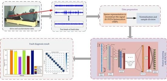
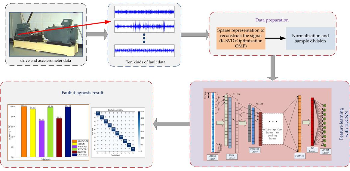
The intelligent fault diagnosis method of rotating machinery based on adaptive learning dictionary and 1DCNN proposed in this paper is as follows: firstly, the adaptive learning dictionary is constructed by K-SVD algorithm, the collected vibration signal is sparsely represented by orthogonal matching pursuit algorithm, and the reconstructed signal is obtained; secondly, the reconstructed signal is normalized and divided into a training set, test set, and verification set. Finally, input the training set into the 1DCNN network model for training; then, use cross-validation to select the optimal model through the verification set, and then evaluate the performance of the model through the test set to complete the fault diagnosis task. The specific method flow is shown in Figure 3, and the details are as follows:
- (1)
- The original vibration signal collected by the sensor is sparsely represented and normalized, and the training set, verification set, and test set are divided according to a certain proportion.
- (2)
- Construct one-dimensional convolution neural network and set relevant network parameters: iterative steps, training batches, convolution layers, and convolution kernel size, number, and step size of each layer.
- (3)
- Initialize the network parameters, input the training samples into the 1DCNN network in batches, and begin to perform the forward propagation of the model. The output layer obtains the accuracy and calculates the error.
- (4)
- Carry on the back propagation algorithm to the error, update the weight, and offset until the network training is completed.
- (5)
- Input the test set into the trained model, output the classification accuracy, and evaluate the classification effect.
5. Experiment Verification and Analysis
In order to test the performance of the fault diagnosis method proposed in this paper and verify its effectiveness, experiments are carried out with two different datasets: the bearing dataset of CWRU and the worm gear reducer dataset of Shanghai University of Technology, which are compared with other traditional intelligent diagnosis methods.
5.1. Experiment on Datasets of Rolling Bearing in Case Western Reserve University
5.1.1. Experiment Description
The experimental data are from the bearing database of CWRU [42]. The experimental bearing type is deep groove ball bearing SKF6205. In this experiment, the mixed data under four kinds of load of drive end bearing 0–3 hp are selected. The bearing experimental platform is shown in Figure 4. A 16-channel acquisition instrument is selected to collect vibration signals, and the sampling frequency is 12 kHz. Three kinds of defect positions of bearings are machined by electro-discharge machining (EDM), which are the ball fault (B), outer race fault (OR), and inner race fault (IR). Each type of damage has three sizes: 0.007 inches, 0.014 inches, and 0.021 inches. Bearings with different fault locations and different degrees of damage are regarded as a separate category, including a total of 10 bearing types in the normal state. Data enhancement is used to construct 1000 samples for each type of signal features, and one-hot coding [43] is used to label ten types of bearing states. The experimental dataset is divided into a training set, verification set, and test set according to 6:1:3, and the dataset and samples are divided as shown in Table 1.
The original time-domain waveforms of vibration signals in 10 types of rolling bearings are shown in Figure 5. According to the figure, it is difficult to judge the fault types of rolling bearings by time-domain analysis, so this paper uses a sparse representation method to sparsely decompose the original signal in each state, extract effective features, and then reconstruct the signal. Finally, combined with 1DCNN, 10 kinds of faults of rolling bearings are classified and diagnosed.
5.1.2. Optimization Selection of the SR−1DCNN Model
- (1)
- Sparse representation selection of related parameters
In the process of sparse representation, the sparsity of the original vibration signal is determined by setting the parameter sparsity k in the OMP algorithm. If the parameter k is too large, the sparse component will contain too many signal features; while if the parameter k is too small, it will lead to the loss of some feature information. In addition, in the process of learning the construction of dictionary D, a small number of atoms will lead to fewer fault features in the reconstructed signal, while too many atoms will cause more noise interference in the reconstructed signal, which cannot achieve the effect of noise reduction. At the same time, in the process of adaptive dictionary training and learning, the selection of sample length W determines the number of training samples, which will also affect the impact feature information contained in the reconstructed signal. Therefore, the parameters are adjusted by reconstructing the relationship between the signal envelope kurtosis and the parameters. For example, Figure 6 shows the rolling body fault and the relationship between the sparsity and the reconstruction signal envelope kurtosis when the damage diameter is 0.007 inches. In order to ensure the maximum retention of the impact characteristic components of the reconstructed signal and highlight the characteristics of the impact fault, the sparse degree is finally selected. The same selection criteria select other sparse representation parameters in the fault state and finally choose the sample length Wend64; the number of atoms is 1024. The state of ten kinds of bearings are sparsely represented and reconstructed signals.
- (2)
- Parameter selection of 1DCNN Network Model
The structure of the 1DCNN model used in this paper is modified based on WDCNN [44]. The accuracy and loss are obtained by adjusting the number of network layers and the size, number, and step size of the convolution kernel, and the final selected network model parameters are shown in Table 2. The training and learning design of the 1DCNN-based network model consists of five convolution stages for feature extraction; each convolution stage contains a set of one-dimensional convolution layers for learning important features from the input signal, and the batch normalization layer normalizes a batch output feature vector to an appropriate data distribution, which makes the value of the intermediate output of each layer more stable, thus accelerating the learning speed of the model. The nonlinear element activation function (Relu) is used for nonlinear transformation of the extracted features to overcome the problem of gradient disappearance and speed up the training speed, and the maximum pool layer is used to improve the local translation invariance of the input signal features. The first convolution layer in the network model uses a wide convolution core to suppress the high-frequency noise in the input signal and capture the correlation with the distance, while the other convolution layer uses a smaller convolution kernel to obtain a complex representation of the characteristics of the input signal. The output layer has 10 neurons to classify 10 health states of the bearing.
5.1.3. Data Enhancement
The network model used in this paper is 1DCNN, and the input reconstructed signal is a one-dimensional time series signal. The prerequisite for this kind of deep learning model is to use a lot of data to train the model in order to enhance the generalization ability of the model. However, in the actual operation of the machine, due to the fault, it is very difficult for the machine to run for a long time, and a large amount of data can rarely be collected. Therefore, data enhancement technology is also widely used in convolution neural networks, and higher classification accuracy can be obtained in the case of fewer fault samples. Among them, through the overlapping method to intercept the training samples, it is easier to obtain a large amount of data. By setting the offset and sample length, the vibration signals under different fault types are overlapped and sampled by the method of equal interval offset sliding, so as to increase the number of training samples. The schematic diagram is shown in Figure 7.
5.1.4. Analyze the Process and Results
Figure 8 shows the classification accuracy and loss function values of the training set and verification set after 50 rounds of iterations in 1DCNN using the method proposed in this paper. Through the analysis of the accuracy and loss change curve, it can be seen that when the model is trained to the fourth time, the accuracy reaches a large value, and the accuracy fluctuates less in the subsequent training process, indicating that the network model training has been completed. The trained network model is tested with test samples, and the accuracy of the final test set is 99.67%. The experimental results show that the proposed model has few iterations, high convergence accuracy, and small loss, which shows that the network model designed by this method is reasonable.
In order to show the recognition results of each category of the model in the test set more clearly, the confusion matrix is introduced to analyze the experimental results in detail, as shown in Figure 9, where 0–9 represent 10 states of the rolling bearing, respectively, and their representation labels are shown in Table 1. The X-axis represents the predicted category label of the fault, the Y-axis represents the real category label of the fault, the dark area on the diagonal of the figure represents the accuracy corresponding to each type of fault, 300 represents the number of test sets for each type of fault, and the values in other areas are the number of misclassification. As shown in the confusion matrix, the value of the corresponding position of real Category 4 and Predictive Category 1 is 1, which indicates that one test Category 4 is misclassified as Fault Category 1; that is, one 0.007-inch inner fault is misclassified to a rolling ball fault with a damage diameter of 0.007 inches. It can be seen from the diagram that except for the classification accuracy of test category 4 (IR007), the other nine fault types can be classified accurately, indicating that the combination of sparse representation and 1DCNN proposed in this paper can achieve satisfactory classification results in fault classification and diagnosis, and it has great feasibility.
In the actual working conditions, the measured bearing vibration signals are often mixed with the interference of a large number of noise signals, so the robustness and generalization ability of a 1DCNN model under different noise interferences are studied. The method was used to carry out 10 tests, and the accuracy of the test set was output, respectively. In the first experiment, Gaussian white noise with different SNRs was added to all 3000 test samples to simulate the influence of noise on the results of classification diagnosis under real working conditions. The definition of SNR is shown in Formula (6), and the trained 1DCNN model is used to test the accuracy of the noisy-adding test set.
where represents the power of the original signal and represents the power of the noise signal. The smaller the SNR, the greater the noise interference.
According to the data obtained from 10 experiments in Figure 10, the average accuracy of the model based on this method for rolling bearing fault diagnosis is 99.82%, with the highest accuracy of 99.96% and the lowest accuracy of 99.56%. The results of 10 experiments show that the model based on the method adopted in this paper has good robustness in fault classification and identification of rolling bearings.
The classification accuracy of the test set under different SNRs is shown in Figure 11. After the noise interference of different SNRs is added to the test sample, the model can still quickly learn the characteristics of the data. When SNR <0 dB, the accuracy of the model is low, when SNR >4 dB, its accuracy is higher than 95%, and the resolution of different SNR noise based on the method proposed in this paper is higher than that of the model that classifies the original signal directly. It can be seen that based on the model used in this method, the model can maintain high accuracy under noise interference, and it has strong anti-noise stability and generalization ability.
In order to further verify the effectiveness of the bearing diagnosis method based on sparse representation and 1DCNN, the method model used in this paper is compared with the following bearing fault diagnosis methods based on traditional machine learning classification, including the one-dimensional convolution neural network (1DCNN) model, wavelet packet decomposition + convolution neural network (WPD-CNN) model in reference [45], convolution neural network + support vector machine (CNN-SVM) model based on adaptive features in reference [46], a new data-driven fault diagnosis method-based Wen-CNN model proposed by Wen in reference [21], and a rotating machinery fault diagnosis method (ResCNN) model based on deep residual learning in reference [47].
The comparison between the method used in this paper and other fault classification methods is shown in Figure 12. It can be seen from the figure that the diagnosis model based on sparse representation and the 1DCNN method can effectively extract fault features and accurately classify bearing faults, it has a higher accuracy, and the diagnosis effect is more significant than other methods.
5.2. Dataset Experiment of Worm Gear Reducer
5.2.1. Experimental Description
The dataset of a worm gear reducer is from the experimental database of the Shanghai University of Science and Technology [48]; the type of worm gear reducer is WPA40, the deceleration ratio is 1:10, the worm head number is 2, the worm gear tooth number is 20, the worm gear indexing circle diameter is 30 mm, the modulus is 2 m, the lead angle is 9°28′, and the pressure angle is 20°. Two AC servo motors are used to load and drive respectively, and the load size is 0 Nm or 6 Nm. Artificial faults are added to the worm gear, which are pitting, spalling, and breaking, respectively. The sensor uses a three-axis accelerometer, which can collect vibration signals in three orthogonal directions at the same time, which is installed on the gearbox body with a sampling frequency of 12.8 kH, and the fault experimental platform is shown in Figure 13. In this experiment, the vibration signal in the X-axis direction, which is most sensitive to the vibration caused by the worm gear fault, is selected as the analysis signal source. The servo motor speed is 1000 rpm, the mixed data with a load of 0 Nm and 6 Nm are selected, and four types of fault modes including normal state are selected, which are normal (NOR), pitting (PIT), spalling (SPA), and breaking (BRO). The length of each sample is 2048, the number of samples for each type of fault is 1000, and the training set, verification set, and test set are divided according to 6:1:3. For example, Table 3 shows the details of the experimental dataset. Figure 14 shows the original waveform of the vibration signal measured in the four states of the worm gear.
5.2.2. Analysis Process and Results
Figure 15 show that when the number of trainings is about five times, the network model has tended to be stable, and the accuracy of the test set has reached 99.83%. The results show that the network model based on this method is also applicable to the experimental dataset of the worm gear reducer.
As shown in Figure 16, the multi-class confusion matrix of the result is obtained for the first time by this method. The results show that the overall diagnostic accuracy of the four categories was 99.83%, and the error rate is 0.17%. Among them, two samples in category 3 are misclassified to category 0; that is, two samples of broken teeth are misclassified to normal faults, and there is only one misclassification, and the classification effect is satisfactory.
In order to evaluate the fault identification ability of the proposed model, the network model is used to carry out 10 fault classification experiments on the dataset, and the test results are shown in Figure 17. The average accuracy of 10 experiments is 99.76%, the highest accuracy is 99.93%, and the lowest accuracy is 99.56%. The results show that this method has more reliable performance.
As can be seen in Figure 18, the accuracy of the SR-1DCNN fault diagnosis model proposed in this paper for worm gear faults under low SNR is significantly higher than that of the model that classifies the original signals directly. The classification accuracy of the model is 35.6% when SNR = −4 dB. When the signal-to-noise ratio is changed to 6 dB, the accuracy can reach more than 90%. It can still maintain a high accuracy in the presence of noise, which proves the effectiveness of the model for worm gear fault diagnosis in noisy environment.
Figure 19 shows the classification performance comparison results of different methods. In this experiment, four types of worm gear fault data composed of 0 Nm and 6 Nm under four fault states are used. Compared with reference [48] SFDSC and reference [49] SISC, experiments were carried out under two loads of SISC, SFDSC0 Nm and 6 Nm, each with four types of data, in which the diagnosis accuracy of the 0 Nm load was higher than that of the 6 Nm load, reaching 90.56% and 96.67% respectively, while the classification accuracy of this method reached 99.76%, which was higher than that of the above two models. The results show that the method proposed can effectively extract fault features and has high classification accuracy.
6. Discussion
In practical engineering, the vibration signals actually measured by sensors often contain lots of noise interference, which greatly increase the difficulty of extracting fault features by the 1DCNN model. In this paper, the original signal is preprocessed denoised to improve the diagnosis accuracy. That is, sparse representation preprocessing and denoising of the original signal requires the manual removal of noise components in the signal, and the reconstructed signal after denoising is used as the input of 1DCNN. However, the effect of this method depends on people’s experience to a great extent. That is, there is a need for a rational choices of parameters, such as sparsity k, the size of dictionary atoms, and the length of samples. If the parameters are not selected properly, the reconstructed signal will lose some useful features after denoising, and it is difficult to get the best denoising effect. In this paper, the relevant parameters are adjusted by calculating the envelope spectrum kurtosis of the reconstructed signal. However, it is not guaranteed that denoising is accompanied by the removal of useful signal components, thus affecting the classification accuracy of faults. The final classification accuracy cannot be guaranteed to be the best classification that this method can achieve.
Secondly, preprocessing denoising and feature extraction are two mutually independent processes. After the original signal is denoised by sparse representation, the reconstructed signal is used as the input of 1DCNN, which needs different processing methods. Although the classification accuracy of faults is improved, the workload is also increased.
In addition, the classification accuracy of the method used in this paper has been significantly improved compared with the classification accuracy of the original signal without preprocessing under different SNR. However, in the case of large noise interference, the fault classification accuracy is not very high. For example, when SNR= −4 dB, the classification accuracy of the two sets of datasets can only reach 46.84% and 35.6%, and its classification effect is still a great challenge. The author will study these problems carefully in his future work.
7. Conclusions
For the classification and detection of rotating machinery faults, this paper proposes a method of combining adaptive learning dictionary with 1DCNN, which realizes the effective classification and diagnosis of different fault types of rotating machinery under noise interference. The main conclusions are as follows:
Aiming at the noise reduction of sparse representation preprocessing, an adaptive learning dictionary is constructed by using the K-SVD algorithm; the original signal is sparsely decomposed and reconstructed by the optimized OMP algorithm, the feature signal is extracted effectively, and the signal is reconstructed to reduce the influence of noise. Then, the preprocessed signal is adaptively extracted from deeper signal features by 1DCNN, and the fault is classified. Finally, the classification accuracy of the two groups of experimental data reaches 99.82% and 99.76%, respectively. Compared with other machine learning methods, the results show that the proposed method is effective and feasible for fault classification and the diagnosis of rotating machinery parts such as rolling bearings and worm gears.
The SR-1DCNN network model proposed in this paper has fast convergence speed and strong robustness in the test of the Case Western Reserve University (CWRU) rolling bearing database and worm gear reducer dataset. The noise environment interference with a different SNR is added to the test set to simulate the influence of noise on the classification accuracy in the actual industrial environment. The experimental results show that this method can well identify the faults of rotating machinery such as bearings and worm gears. It is verified that the model has good generalization ability and strong anti-noise ability.
In the future work, the author will further study the method based on the combination of preprocessing denoising and network feature extraction and classification. Through the study of the existing technology, we can avoid or reduce the possible impact on the classification accuracy caused by manual processing as much as possible. In addition, in the case of very large noise interference, the classification accuracy is not very good, which may be due to the loss of some features due to sparse representation noise reduction, which affects the classification accuracy. We will study a better evaluation standard.
Author Contributions
Conceptualization, H.W. and C.L.; methodology, H.W. and C.L.; software, H.W. and C.L.; validation, H.W., C.L. and W.D.; formal analysis, C.L.; investigation, C.L.; resources, H.W., W.D. and S.W.; data curation, H.W. and C.L.; writing—original draft preparation, C.L.; writing—review and editing, C.L., H.W. and W.D.; visualization, C.L.; supervision, H.W., W.D. and S.W.; project administration, H.W. and C.L.; funding acquisition, W.D. All authors have read and agreed to the published version of the manuscript.
Funding
The research is supported by the National Natural Science Foundation of china (approved grant: U1804141).
Data Availability Statement
Publicly available datasets [42] were analyzed in this study, other datasets are proprietary and cannot be shared at this time.
Conflicts of Interest
The authors declare no conflict of interest.
References
- Wang, Z.J.; Zhou, J.; Wang, J.Y.; Du, W.H.; Wang, J.T.; Han, X.F.; He, G.F. A novel fault diagnosis method of gearbox based on maximum kurtosis spectral entropy deconvolution. IEEE Access 2019, 7, 29520–29532. [Google Scholar] [CrossRef]
- Xu, Y.; Li, Z.X.; Wang, S.Q.; Li, W.H.; Thompson, S.G.; Feng, S.Z. A Hybrid Deep-Learning Model for Fault Diagnosis of Rolling Bearings. Measurement 2021, 169, 108502. [Google Scholar] [CrossRef]
- Wu, J.; Wu, C.Y.; Cao, S.; Or, S.W.; Deng, C.; Shao, X.Y. Degradation data-driven time-to-failure prognostics approach for rolling element bearings in electrical machines. IEEE Trans. Ind. Electron. 2019, 66, 529–539. [Google Scholar] [CrossRef]
- Cerrada, M.; Sánchez, R.V.; Li, C.; Pacheco, F.; Cabrera, D.; Oliveira, J.V.D.; Vásquez, R.E. A review on data-driven fault severity assessment in rolling bearings. Mech. Syst. Signal Process. 2018, 99, 169–196. [Google Scholar] [CrossRef]
- Jiang, G.Q.; He, H.B.; Yan, J.; Xie, P. Multiscale convolutional neural networks for fault diagnosis of wind turbine gearbox. IEEE Trans. Ind. Electron. 2018, 66, 3196–3207. [Google Scholar] [CrossRef]
- Xiao, M.H.; Wen, K.; Zhang, C.Y.; Zhao, X.; Wei, W.H.; Wu, D. Research on Fault Feature Extraction Method of Rolling Bearing Based on NMD and Wavelet Threshold Denoising. Shock. Vib. 2018, 2018, 9495265. [Google Scholar] [CrossRef]
- Abdelkader, R.; Kaddour, A.; Derouiche, Z. Enhancement of rolling bearing fault diagnosis based on improvement of empirical mode decomposition denoising metho. Int. J. Adv. Manuf. Technol. 2018, 97, 3099–3117. [Google Scholar] [CrossRef]
- Wang, P.; Wang, T.Y. Energy weighting method and its application to fault diagnosis of rolling bearing. J. Vibroeng. 2017, 19, 223–236. [Google Scholar] [CrossRef]
- Alexakos, C.T.; Karnavas, Y.L.; Drakaki, M.; Tziafettas, I.A. A Combined Short Time Fourier Transform and Image Classification Transformer Model for Rolling Element Bearings Fault Diagnosis in Electric Motors. Mach. Learn. Knowl. Extr. 2021, 3, 11. [Google Scholar] [CrossRef]
- Yi, Q. A New Family of Model-Based Impulsive Wavelets and Their Sparse Representation for Rolling Bearing Fault Diagnosis. IEEE Trans. Ind. Electron. 2018, 65, 2716–2726. [Google Scholar]
- Wang, L.; Cai, G.G.; Gao, G.Q.Z.F.; Yang, S.Y.; Zhu, Z.K. Fast algorithm of sparse representation based on improved MP and its application of rolling bearing fault feature extraction. Vib. Shock. 2017, 36, 176–182. [Google Scholar]
- Hou, F.T.; Chen, J.; Dong, G.M. Weak fault feature extraction of rolling bearings based on globally optimized sparse coding and approximate SVD. Mech. Syst. Signal Process. 2018, 111, 234–250. [Google Scholar] [CrossRef]
- Li, J.M.; Li, M.; Yao, X.F.; Wang, H.; Yu, Q.W.; Wang, X.D. Rolling bearing fault diagnosis based on ensemble empirical mode decomposition and k-singular value decomposition dictionary learning. Acta Metrol. Sin. 2020, 41, 1260–1266. [Google Scholar]
- Yang, H.G.; Lin, H.B.; Ding, K. Sliding window denoising K-Singular Value Decomposition and its application on rolling bearing impact fault diagnosis. J. Sound Vib. 2018, 421, 205–219. [Google Scholar] [CrossRef]
- Zeng, M.; Zhang, W.M.; Chen, Z. Group-Based K-SVD Denoising for Bearing Fault Diagnosis. IEEE Sens. J. 2019, 99, 1. [Google Scholar] [CrossRef]
- Lu, W.; Song, L.Y.; Cui, L.L.; Wang, H.Q. A Novel Weak Fault Diagnosis Method Based on Sparse Representation and Empirical Wavelet Transform for Rolling Bearing. In Proceedings of the 2020 International Conference on Sensing, Measurement & Data Analytics in the era of Artificial Intelligence (ICSMD), Xi’an, China, 15–17 October 2020. [Google Scholar]
- Wang, Z.Y.; Yao, L.G.; Cai, Y.W. Rolling bearing fault diagnosis using generalized refined composite multiscale sample entropy and optimized support vector machine. Measurement 2020, 156, 107574. [Google Scholar] [CrossRef]
- Wang, H.Y.; Yu, Z.Q.; Guo, L. Real-time Online Fault Diagnosis of Rolling Bearings Based on KNN Algorithm. J. Phys. Conf. Ser. 2020, 1486, 032019. [Google Scholar] [CrossRef]
- Li, J.M.; Yao, X.F.; Wang, X.D.; Yu, Q.W.; Zhang, Y.G. Multiscale local features learning based on BP neural network for rolling bearing intelligent fault diagnosis. Measurement 2020, 153, 107419. [Google Scholar] [CrossRef]
- Peng, D.D.; Wang, H.; Liu, Z.L.; Zhang, W.; Zuo, M.J.; Chen, J. Multi-branch and Multi-scale CNN for Fault Diagnosis of Wheelset Bearings under Strong Noise and Variable Load Condition. IEEE Trans. Ind. Inform. 2020, 16, 4949–4960. [Google Scholar] [CrossRef]
- Wen, L.; Li, X.Y.; Gao, L.; Zhang, Y.Y. A New Convolutional Neural Network-Based Data-Driven Fault Diagnosis Method. IEEE Trans. Ind. Electron. 2018, 65, 5990–5998. [Google Scholar] [CrossRef]
- Li, H.; Zhang, Q.; Qin, X.R.; Sun, Y.T. Fault diagnosis method for rolling bearings based on short-time Fourier transform and convolutional neural network. J. Vib. Shock. 2018, 37, 124–131. [Google Scholar]
- Liu, R.N.; Wang, F.; Yang, B.Y.; Qin, S.J. Multiscale Kernel Based Residual Convolutional Neural Network for Motor Fault Diagnosis Under Nonstationary Conditions. IEEE Trans. Ind. Inform. 2020, 16, 3797–3806. [Google Scholar] [CrossRef]
- Yang, Y.H.; Li, D.L.; Liu, X.Z. Fault Diagnosis Based On One-Dimensional Deep Convolution Neural Network. In Proceedings of the 2020 Chinese Control and Decision Conference (CCDC) IEEE, Hefei, China, 22–24 August 2020. [Google Scholar]
- Zhang, A.S.; Li, S.B.; Cui, Y.X.; Yang, W.; Dong, R.; Hu, J. Limited Data Rolling Bearing Fault Diagnosis With Few-Shot Learning. IEEE Access 2019, 7, 110895–110904. [Google Scholar] [CrossRef]
- Qin, C.J.; Jin, Y.R.; Tao, J.F.; Yang, W.L.; Dong, R.Z.; Hu, J.J. DTCNNMI: A deep twin convolutional neural networks with multi-domain inputs for strongly noisy diesel engine misfire detection. Measurement 2021, 180, 109548. [Google Scholar] [CrossRef]
- Xue, Y.; Dou, D.Y.; Yang, J.G. Multi-fault diagnosis of rotating machinery based on deep convolution neural network and support vector machine. Measurement 2020, 156, 107571. [Google Scholar] [CrossRef]
- Ji, M.Y.; Peng, G.L.; He, J.; Liu, S.H.; Chen, Z.; Li, S.J. A Two-Stage, Intelligent Bearing-Fault-Diagnosis Method Using Order-Tracking and a One-Dimensional Convolutional Neural Network with Variable Speeds. Sensors 2021, 21, 675. [Google Scholar] [CrossRef]
- Peng, D.D.; Liu, Z.L.; Wang, H.; Qin, Y.; Jia, L.M. A novel deeper one-dimensional CNN with residual learning for fault diagnosis of wheelset bearings in high-speed trains. IEEE Access 2018, 7, 10278–10293. [Google Scholar] [CrossRef]
- He, K.M.; Sun, J. Convolutional neural networks at constrained time cost. In Proceedings of the 2015 IEEE Conference on Computer Vision and Pattern Recognition (CVPR), Boston, MA, USA, 7–12 June 2015; pp. 5353–5360. [Google Scholar]
- He, K.M.; Zhang, X.Y.; Ren, S.Q.; Sun, J. Deep Residual Learning for Image Recognition. In Proceedings of the 2016 IEEE Conference on Computer Vision and Pattern Recognition (CVPR), Las Vegas, NV, USA, 27–30 June 2016; pp. 770–778. [Google Scholar]
- Olshausen, B.A.; Field, D.J. Emergence of imple-cell receptive field properties by learning a sparse code for natural images. Nature 1996, 381, 607–609. [Google Scholar] [CrossRef] [PubMed]
- Zhang, J.; Zhao, C.; Zhao, D.B.; Gao, W. Image compressive sensing recovery using adaptively learned sparsifying basis via L0 minimization. Signal Process. 2014, 103, 114–126. [Google Scholar] [CrossRef] [Green Version]
- Aharon, M.; Elad, M.; Bruckstein, A. K-SVD: An Algorithm for Designing Overcomplete Dictionaries for Sparse Representation. IEEE Trans. Signal Process. 2006, 54, 4311–4322. [Google Scholar] [CrossRef]
- Tropp, J.A.; Gilbert, A.C. Signal Recovery from Random Measurements Via Orthogonal Matching Pursuit. IEEE Trans. Inf. Theory 2007, 53, 4655–4666. [Google Scholar] [CrossRef] [Green Version]
- Wang, L.; Cai, G.G.; You, W.; Huang, W.G.; Zhu, Z.K. Transients Extraction Based on Averaged Random Orthogonal Matching Pursuit Algorithm for Machinery Fault Diagnosis. IEEE Trans. Instrum. Meas. 2017, 66, 3237–3248. [Google Scholar] [CrossRef]
- Tang, S.G.; Yuan, S.Q.; Zhu, Y. Convolutional Neural Network in Intelligent Fault Diagnosis toward Rotatory Machinery. IEEE Access 2020, 8, 86510–86519. [Google Scholar] [CrossRef]
- Liang, P.F.; Deng, C.; Wu, J.; Yang, Z.X. Intelligent fault diagnosis of rotating machinery via wavelet transform, generative adversarial nets and convolutional neural network. Measurement 2020, 159, 107768. [Google Scholar] [CrossRef]
- Goodfellow, I.; Bengio, Y.; Courville, A. Deep Learning; MIT Press: Cambridge, MA, USA, 2016. [Google Scholar]
- Ide, H.; Kurita, T. Improvement of learning for CNN with ReLU activation by sparse regularization. In Proceedings of the 2017 International Joint Conference on Neural Networks (IJCNN), Anchorage, AK, USA, 14–19 May 2017; pp. 2684–2691. [Google Scholar]
- Huang, S.Z.; Tang, J.; Dai, J.Y.; Wang, Y.Y.; Dong, J.J. 1DCNN Fault Diagnosis Based on Cubic Spline Interpolation Pooling. Shock. Vib. 2020, 2020, 1949863. [Google Scholar] [CrossRef] [Green Version]
- Case Western Reserve University Bearing Data Center. Available online: https://csegroups.case.edu/bearingdatacenter/home (accessed on 15 August 2021).
- Akata, Z.; Perronnin, F.; Harchaoui, Z.; Schmid, C. Label-Embedding for Image Classification. IEEE Trans. Pattern Anal. Mach. Intell. 2016, 38, 1425–1438. [Google Scholar] [CrossRef] [Green Version]
- Zhang, W.; Peng, G.L.; Li, C.H.; Chen, Y.H.; Zhang, Z.J. A new deep learning model for fault diagnosis with good anti-noise and domain adaptation ability on raw vibration signals. Sensors 2017, 17, 425. [Google Scholar] [CrossRef]
- Chen, L.L.; Fu, Z.C.; Ling, J.; Dong, S.J. Fault diagnosis of rolling bearing based on WPD-CNN two-dimensional time-frequency image. Modul. Mach. Tool Autom. Mach. Technol. 2021, 3, 57–61. [Google Scholar]
- Han, T.; Zhang, L.W.; Yin, Z.J.; Tan, A.C.C. Rolling bearing fault diagnosis with combined convolutional neural networks and support vector machine. Measurement 2021, 177, 109022. [Google Scholar] [CrossRef]
- Zhang, W.; Li, X.; Ding, Q. Deep residual learning-based fault diagnosis method for rotating machinery. ISA Trans. 2019, 95, 295–305. [Google Scholar] [CrossRef]
- Wang, S.Y. Research on Key Technologies of Wind Turbine Health Monitoring and Evaluation; Shanghai Jiaotong University: Shanghai, China, 2017. [Google Scholar]
- Liu, H.N.; Liu, C.L.; Huang, Y.X. Adaptive feature extraction using sparse coding for machinery fault diagnosis. Mech. Syst. Signal Process. 2011, 25, 558–574. [Google Scholar] [CrossRef]
Figure 1.
K-SVD algorithm flow.

Figure 2.
Schematic diagram of 1DCNN process.

Figure 3.
Fault diagnosis process based on adaptive learning dictionary and 1DCNN.

Figure 4.
CWRU bearing fault test rig [42].
Figure 4.
CWRU bearing fault test rig [42].

Figure 5.
Original vibration signal time-domain waveforms of the drive-end rolling bearing under the 0–3 hp load.
Figure 5.
Original vibration signal time-domain waveforms of the drive-end rolling bearing under the 0–3 hp load.

Figure 6.
Relationship between sparsity and reconstructed signal envelope spectral kurtosis.

Figure 7.
Data augmentation with overlap.

Figure 8.
(a) Accuracy of the SR-1DCNN model; (b) Loss of the SR-1DCNN model.

Figure 9.
Confusion matrix of the SR-1DCNN model (test set of CWRU).

Figure 10.
Accuracy of ten experiments (test set of CWRU).

Figure 11.
Accuracy of test set under different SNR (test set of CWRU).

Figure 12.
Comparison of different methods (test set of CWRU).

Figure 13.
Worm gear fault test rig.

Figure 14.
Original vibration signal time-domain waveforms of worm gear.

Figure 15.
(a) Accuracy of the SR−1DCNN model; (b) Loss of the SR−1DCNN model.

Figure 16.
Confusion matrix of the SR-1DCNN model (test set of Worm Gear Reducer).

Figure 17.
Accuracy of ten experiments (test set of Worm Gear Reducer).

Figure 18.
Accuracy of test set under different SNR (test set of Worm Gear Reducer).

Figure 19.
Comparison of different methods (test set of Worm Gear Reducer).


Table 1.
Description of the rolling bearing dataset and sample partition.
| Fault Location | Normal | Ball (B) | Inner Race (IR) | Outer Race (OR) | ||||||
|---|---|---|---|---|---|---|---|---|---|---|
| Category labels | 0 | 1 | 2 | 3 | 4 | 5 | 6 | 7 | 8 | 9 |
| Fault diameter | 0 | 0.007 | 0.014 | 0.021 | 0.007 | 0.014 | 0.021 | 0.007 | 0.014 | 0.021 |
| Sample length | 2048 | 2048 | 2048 | 2048 | 2048 | 2048 | 2048 | 2048 | 2048 | 2048 |
| Load (hp) | 0,1,2,3 | 0,1,2,3 | 0,1,2,3 | 0,1,2,3 | 0,1,2,3 | 0,1,2,3 | 0,1,2,3 | 0,1,2,3 | 0,1,2,3 | 0,1,2,3 |
| Training sample | 600 | 600 | 600 | 600 | 600 | 600 | 600 | 600 | 600 | 600 |
| Validation sample | 100 | 100 | 100 | 100 | 100 | 100 | 100 | 100 | 100 | 100 |
| Testing sample | 300 | 300 | 300 | 300 | 300 | 300 | 300 | 300 | 300 | 300 |
Table 2.
The parameters of the constructed 1DCNN.
| Network Layer | Kernel Number | Kernel Size | Kernel Stride |
|---|---|---|---|
| Convolution layer 1 | 16 | 16 | 2 |
| Pooling layer 1 | 16 | 2 | 2 |
| Convolution layer 2 | 32 | 3 | 1 |
| Pooling layer 2 | 32 | 2 | 2 |
| Convolution layer 3 | 64 | 3 | 1 |
| Pooling layer 3 | 64 | 2 | 2 |
| Convolution layer 4 | 64 | 3 | 1 |
| Pooling layer 4 | 64 | 2 | 2 |
| Convolution layer 5 | 64 | 3 | 1 |
| Pooling layer 5 | 64 | 2 | 2 |
| Fully connection | 1 | 100 | — |
| Softmax | 1 | 10 | — |
Table 3.
Description of the worm gear dataset and sample partition.
| Fault Location | Normal | Pitting | Spalling | Breaking |
|---|---|---|---|---|
| Category labels | 0 | 1 | 2 | 3 |
| Sample length | 2048 | 2048 | 2048 | 2048 |
| Load (Nm) | 0.6 | 0.6 | 0.6 | 0.6 |
| Training sample | 600 | 600 | 600 | 600 |
| Validation sample | 100 | 100 | 100 | 100 |
| Testing sample | 300 | 300 | 300 | 300 |
Publisher’s Note: MDPI stays neutral with regard to jurisdictional claims in published maps and institutional affiliations. |
© 2021 by the authors. Licensee MDPI, Basel, Switzerland. This article is an open access article distributed under the terms and conditions of the Creative Commons Attribution (CC BY) license (https://creativecommons.org/licenses/by/4.0/).
Share and Cite
MDPI and ACS Style
Wang, H.; Liu, C.; Du, W.; Wang, S. Intelligent Diagnosis of Rotating Machinery Based on Optimized Adaptive Learning Dictionary and 1DCNN. Appl. Sci. 2021, 11, 11325. https://doi.org/10.3390/app112311325
AMA Style
Wang H, Liu C, Du W, Wang S. Intelligent Diagnosis of Rotating Machinery Based on Optimized Adaptive Learning Dictionary and 1DCNN. Applied Sciences. 2021; 11(23):11325. https://doi.org/10.3390/app112311325
Chicago/Turabian StyleWang, Hongchao, Chuang Liu, Wenliao Du, and Shuangyuan Wang. 2021. "Intelligent Diagnosis of Rotating Machinery Based on Optimized Adaptive Learning Dictionary and 1DCNN" Applied Sciences 11, no. 23: 11325. https://doi.org/10.3390/app112311325
Note that from the first issue of 2016, this journal uses article numbers instead of page numbers. See further details here.