Article

Rolling Bearing Weak Fault Feature Extraction under Variable Speed Conditions via Joint Sparsity and Low-Rankness in the Cyclic Order-Frequency Domain

1
College of Logistics Engineering, Shanghai Maritime University, Shanghai 201306, China
2
Institute of Vibration, Shock and Noise, State Key Laboratory of Mechanical System and Vibration, Shanghai Jiao Tong University, Shanghai 200240, China
*
Author to whom correspondence should be addressed.
Appl. Sci. 2022, 12(5), 2449; https://doi.org/10.3390/app12052449
Submission received: 30 January 2022 / Revised: 24 February 2022 / Accepted: 24 February 2022 / Published: 26 February 2022
(This article belongs to the Special Issue Machine Learning in Vibration and Acoustics)

Abstract

:
Rolling bearings are critical to the normal operation of mechanical systems, which often undergo time-varying working conditions. When the local defects appear on a rolling bearing, the transient impulses will generate and be covered by the strong background noise. Therefore, extracting the rolling bearing weak fault feature with time-varying speed is critical to mechanical system diagnosis. A weak fault feature extraction strategy of rolling bearing under time-varying working conditions is proposed. Firstly, the order-frequency spectral correlation (OFSC) is computed for transferring the measured signal into a higher dimensional space. Then, the joint sparsity and low-rankness constraint is imposed on OFSC to detect the time-varying faulty characteristics. An algorithm in the alternating direction method of multipliers (ADMM) framework is derived. Finally, the enhanced envelope order spectrum (EEOS) is applied to further detect the defective features, which can make the fault features more obvious. The feasibility of the proposed method is confirmed by simulations and an experimental case.

1. Introduction

Rolling bearings are among the most vital rotating elements in a mechanical system (wind turbine [1], centrifuges, helicopters, washing machines, and so on [2,3]), which may be a direct failure for machines breakdown [4]. When rolling bearings are in normal operation, the vibration will generate, caused by raceway waviness, radial play, friction and so on [5,6]. Once the local defects occur, the transient impulses in vibration signals will generate (quite different from the vibration signals in normal operation), covered by a strong background noise [7]. Thus, the vibration-based analysis can be used for the rolling bearing fault diagnosis, and the fault feature extraction task aims to extract the feature of weak transient impulses from the noisy signal, which is valuable for fault diagnosis [8,9,10] and equipment maintenance.
When the rotating speed is stationary, several methods can be used to identify the stable fault characteristic frequency (FCF) to determine the types of faults (inner race, outer race and rollers). Different techniques have been developed to identify the fault types according to different FCFs, like envelope analysis [11] (shift the higher resonance frequency band into a lower fault frequency band to achieve a higher resolution), wavelet analysis [12] (denoise the vibration signal via wavelet decomposition), spectral kurtosis [13,14] (adaptively choose the resonance frequency band via kurtosis), empirical mode decomposition and its development [15,16,17] (denoise the vibration signal via mode decomposition), frequency band entropy [18] (adaptively choose the resonance frequency band via the frequency band entropy), time-frequency analysis (TFA) [19,20] (extract the fault feature in both time domain and frequency domain). Moreover, the time-frequency analysis method can transfer the measured vibration signal into a higher-dimensional space, which can highlight fault characteristics. Yang et al. [21] introduced the sparsity constraint in the time-frequency domain to extract the rolling bearing fault feature. Unfortunately, the weak fault feature is always hidden by the strong background noise, increasing the difficulty of extracting the fault feature in time frequency representation (TFR) [22]. Note that extracting the fault feature via single sparsity in the time frequency domain is hard to achieve a pleasant performance. In order to denoise the TFR, Yu et al. [23] revealed the sparsity of the fault feature and low-rankness of the background noise in the time-frequency domain. The TFR is denoised and the expected fault feature is obtained according to the robust principal component analysis (RPCA) [24]. However, in this case, the fault feature is also low-rank [25,26], not just sparse. If the parameter selection is unreasonable, the obtained fault feature will be confused with the noise component. To tackle this issue, a periodical sparse low-rank model was proposed [27,28] to consider the faulty characteristics in the time-frequency domain as a simultaneously sparse and low-rank component [29]. Actually, most of the abovementioned methods only consider the stable rotating speed conditions and are invalid to variable speed conditions.
When the rolling bearing undergoes the time-varying working condition, the FCFs will also be time-varying. The time-varying FCFs also increase the difficulty of the fault feature extraction task [30]. If the shaft rotating speed can be determined, the measurement can be resampled into the angular domain [31]. Then, the order tracking technique [32] enables the FCFs to be transferred into a fixed order. Thus, the system kinematics of rolling bearings (periodical impulses and modulations) are reflected in the angular domain. Moreover, the system dynamics of the rolling bearings (system resonances) are still shown in the time domain [33]. Along these lines of thought, a concept of angle-time cyclostationary (AT-CS) signal [34] was proposed to describe the rolling bearing fault signal in both time and angular domain. A useful tool named order-frequency spectral correlation (OFSC) [35] was also proposed to transfer the signal into the cyclic order-frequency domain via double Fourier transform, which transfers the angle to cyclic order domain and the time to frequency domain. When calculating the OFSC, the shaft rotating speed is needed and the vibration signal is resampled into the angular domain. Thus, the time-varying FCF in OFSC is transferred into a specific order. By identifying this specific order, the type of fault can be determined. However, like other TFA methods, the specific cyclic order in OFSC will also be interrupted by the strong background noise in real scenarios, where the time-varying fault feature may be difficult to identify. Thus, the problem of how to successfully extract the time-varying rolling bearing fault feature in the heavy interference should be investigated.
In this paper, a weak fault feature extraction strategy of rolling bearing with variable speed is proposed. The measured vibration signal is firstly transformed into the cyclic order-frequency domain, which is analyzed by OFSC. Then, the fault feature contained in the OFSC is extracted according to the joint sparsity and low-rankness model via an ADMM based algorithm. Finally, the EEOS is further used to enhance the extracted fault feature, making the fault feature more obvious to identify. The following are the primary contributions of this paper:
  • The OFSC is calculated by converting the measurement of a rolling bearing with variable speed into the cyclic order-frequency domain. The joint sparsity and low-rankness of the fault feature in OFSC is firstly revealed in this paper, which can be utilized to extract weak fault features of rolling bearings under variable speed conditions;
  • A joint sparsity and low-rankness constraint is imposed on the OFSC to model the fault feature. To optimize the proposed model, an algorithm named ADMM-SLRJEM is developed to extract the fault feature in OFSC.
The rest of this paper is structured as follows. The measurement of a faulty rolling bearing with variable speed is considered, and the corresponding concepts of AT-CS signal are presented in Section 2. Then, the fault feature in OFSC is revealed to possess the joint sparsity and low-rankness and an ADMM based algorithm is derived in Section 3. Finally, in Section 4 and Section 5, The feasibility of the proposed method is confirmed by simulations and an experimental case, respectively.

2. The Signal of Faulty Rolling Bearing with Variable Speed: An Angle-Time Cyclostationary View

2.1. Problem Statement

The most prevalent places for rolling bearing local defaults are the inner race, outer race, and rollers. The measured vibration signal z ( t ) can be considered as the superposition of transient impulses by local defects and background noise as
z ( t ) = x ( t ) + n ( t ) ,
where x ( t ) denotes transient impulses and n ( t ) is the strong background noise. The faulty characteristics detection is devoted to separating the features of x ( t ) from z ( t ) . When the rolling bearing undergoes the time-varying working conditions, the feature of x ( t ) is time-varying as well. Moreover, the background noise n ( t ) is very strong in the real scenarios, i.e., the signal-to-noise ratio (SNR) is very low even negative, which increases the difficulty of the extraction task. Overall, this paper aims to extract the fault features of the rolling bearing with variable speed and heavy interference.

2.2. The Angle-Time Cyclostationarity of the Faulty Bearing with Variable Speed

The vibration signal generated by a rolling bearing with constant speed is typically cyclostationary. However, the transient impulses and the carriers related to time are no longer constant when the rotating speed is time-varying. The system kinematics of rolling bearings (periodical impulses and modulations) is reflected in the angular domain. Moreover, the system dynamics of the rolling bearings (system resonances) are still shown in the time domain. Therefore, the measurement should be evaluated by combining the time domain and angular domain, which can employ the concept of angle-time cyclostationary (AT-CS) signal.
An effective tool for AT-CS signal analysis is called order-frequency spectral, which can transfer the analyzed signal into the (cyclic) order-frequency domain. Due to the periodic characteristics of rolling bearings in the angle domain, which are contained in the process of variable speed rotation, this tool can be used to effectively extract the cyclic orders of the fault characteristics. Let Z denote the measured signal transferred from z ( t ) in the OFSC, which can be decomposed as
Z = X + N ,
where X and N in OFSC are related to x ( t ) and n ( t ) respectively. When the noise N is strong, the expected fault feature may be overwhelmed in Z . Hereafter, the problem can be re-described as how to feasibly extract the time-varying fault feature X from the measurement Z .

2.3. The Calculation of the Order-Frequency Spectral Correlation

The angle-time autocorrelation function (ATCF) R 2 x ( τ , θ ) of x ( t ) can be computed by the Fourier series at cyclic orders i / Θ as
R 2 x ( θ , τ ) = E { x ( t ( θ ) ) x * ( t ( θ ) τ ) } = i R 2 x i ( τ ) e j 2 π i θ Θ ,
where E · is the statistic means, τ represents the time-lag, ( · ) * denotes the complex conjugation, R 2 x i ( τ ) is the angle-time cyclic correlation function and θ ( t ) = 0 t ω ( t ) d t stands for the angular variable with ω the angular frequency. Equation (3) is a periodic function with a cyclic period Θ .
Similar to the spectral correlation (SC), the bispectral counterpart contained in the order-frequency spectral correlation (OFSC) can be obtained by double Fourier transform of ATCF as
S 2 x ( α , f ) = F θ α , τ f R 2 x ( θ , τ ) ,
where R 2 x ( θ , τ ) is the angle-time autocorrelation function, F θ α denotes the Fourier transform from the variable θ to α , f is the spectral frequency and α is the cyclic order. The enhanced envelope order spectrum (EEOS) is also introduced to further highlight the faulty characteristics, and the EEOS is defined as
S x EEOS ( α ) = 1 f 2 f 1 f 1 f 2 S x ( α , f ) d f ,
where f 1 and f 2 are the upper and lower limits of the given spectral frequency band.

3. The Proposed Rolling Bearing Fault Feature Extraction Method under Variable Speed Conditions

The sparsity and low-rankness of the rolling bearing fault feature in the OFSC are first demonstrated in this section. Then, an algorithm in the ADMM framework is derived to optimize the proposed model.

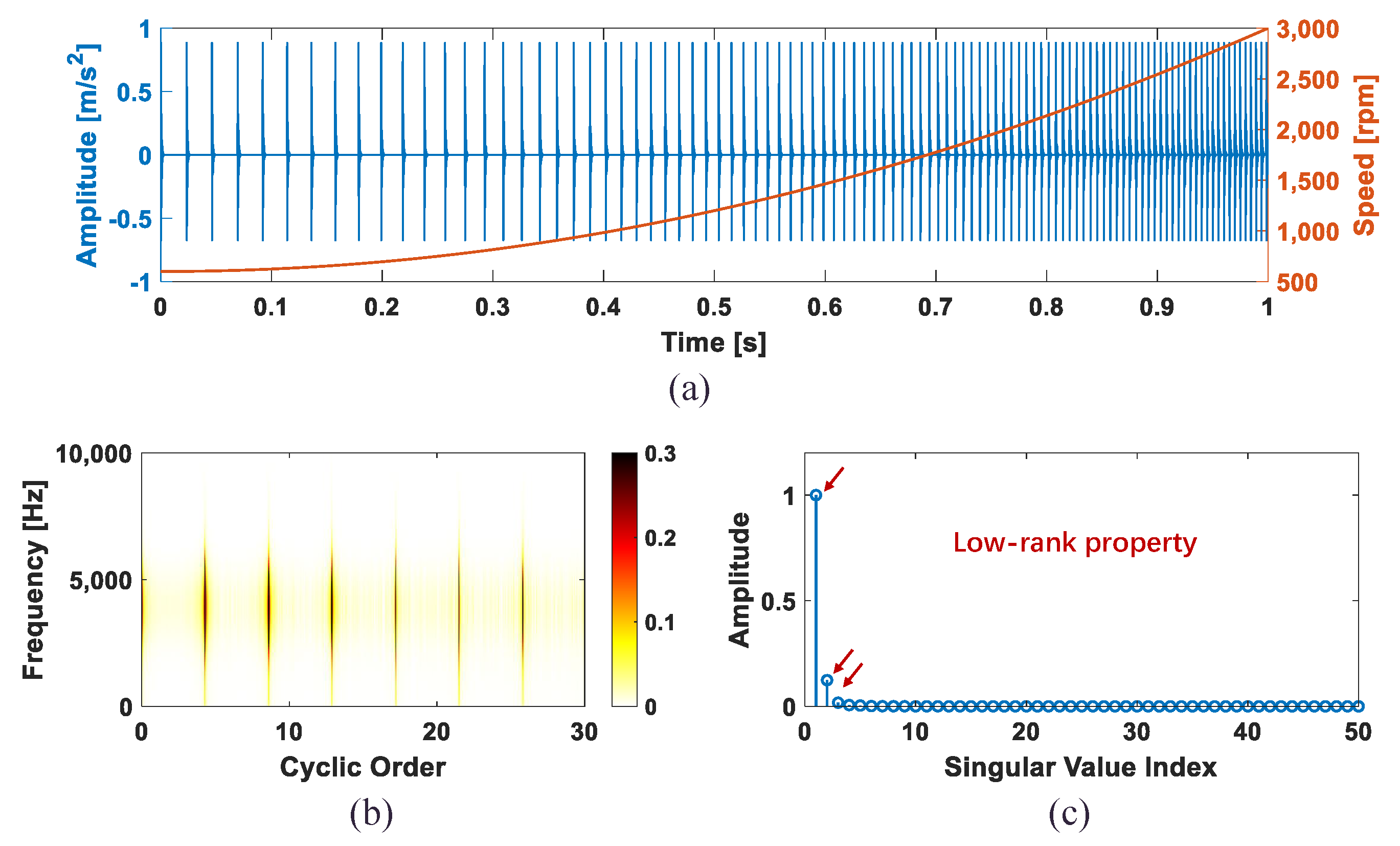
3.1. The Joint Sparsity and Low-Rankness of the Fault Feature in OFSC

In this subsection, a specific example is given to illustrate the sparsity and low-rankness of the faulty rolling characteristics in OFSC. According to the previous study, the faulty rolling bearing signal with variable speed is
z ( t ) = A ( t ) i = 1 L m e β t T i sin 2 π f resonance t T i u ( t T i ) + n ( t ) ,
A ( t ) = 1 + μ cos 2 π 0 t f r ( τ ) d τ ,
where L m represents the impulses count, A ( t ) is the amplitude modification with μ the amplitude modification magnitude, β is the coefficient related to damping, T i is the duration of i-th impulse, u ( t T i ) denotes the step signal with T i as the starting point, and  f resonance is the resonance frequency.
Here, a simulated signal of the outer race fault in a speeding up condition and its OFSC are displayed in Figure 1a,b. The detailed parameters are introduced in Section 4. It can be seen that the intervals between two fault impulses are variable with time. The feature of the fault is sparse in the obtained OFSC. Meanwhile, the singular value decomposition (SVD) is applied on the simulated OFSC, as seen in Figure 1c. It can be seen that the faulty characteristic is relatively large on only several singular values. Hence, the joint sparsity and low-rankness can be used for the extraction of the fault feature.
Combined with Equation (2), the optimization problem of the sparsity and low-rankness jointly enforced X is
minimize X λ 0 X * + λ 1 X L 1 , subject to Z X F δ ,
where λ 0 and λ 1 can be used to adjust the weight of the low-rank and sparse component, · * is the nuclear norm, · L 1 denotes the L 1 norm, · F is the Frobenius norm and δ is the upper bound of the noise N ( N F ). Once the optimazation problem (8) is solved, the joint sparsity and low-rankness fault feature X in the OFSC can be extracted.

3.2. The Optimization Algorithm Derivation

Equation (8) can be further expressed as an unconstrained optimization problem as
minimize X 1 2 Z X F 2 + λ 0 X * + λ 1 X L 1 .
The three terms in Equation (9) are all convex, which means the whole optimization problem is convex and has a globally optimal solution. The ADMM is a high-efficiency computational framework, which allows parallel computing [36]. The convergence of ADMM has been proved in ref. [37]. It can be seen from Equation (9) that the sparsity and low-rankness of the expected fault feature are simultaneously constrained, which makes the optimization more difficult. To decouple the sparsity and low-rankness constraint, an additional constraint X = Y should be introduced, which can be further written as
minimize X , Y 1 2 Z X F 2 + λ 0 Y * + λ 1 X L 1 , subject to X = Y .
Then, the argumented Lagrangian function L is
L ( X , Y , D ) = 1 2 Z X F 2 + ρ 2 X ( Y + D ) F 2 + λ 0 Y * + λ 1 X L 1 ,
where D is the Lagrange multiplier, ρ is the plenty parameter related to the convergence speed. The problem (9) can be solved according to Equation (11) by alternatively solving three sub-problems by iteration as follows:
X ( k + 1 ) = arg min X ( k ) L X ( k ) , Y ( k ) , D ( k ) = arg min X ( k ) 1 2 Z X ( k ) F 2 + ρ 2 X ( k ) Y ( k ) + D ( k ) F 2 + λ 1 X ( k ) L 1 ,
Y ( k + 1 ) = arg min Y ( k ) L X ( k + 1 ) , Y ( k ) , D ( k ) = arg min Y ( k ) ρ 2 X ( k + 1 ) Y ( k ) + D ( k ) F 2 + λ 0 X ( k + 1 ) * ,
D ( k + 1 ) = D ( k ) ( X ( k + 1 ) Y ( k + 1 ) ) ,
where ( · ) k denotes the k-th iteration.

3.2.1. The Solution of Sub-Problem (12)

Combining similar terms and ignoring constant terms (the detailed process can be found in Appendix A), the sub-problem of Equation (12) is rewritten as
X ( k + 1 ) = arg min X ( k ) 1 2 1 1 + ρ Z + ρ Y ( k ) + D ( k ) X ( k ) F 2 + λ 1 1 + ρ X ( k ) L 1 .
To minimize the L 1 norm, the soft-threshold function [38] is used, which can be defined as
soft ( a , T ) = a + T a T 0 | a | T a T a T ,
where a can be regarded as an element in matrix A and T is the threshold. Thus, X ( k + 1 ) can be calculated as
X ( k + 1 ) = soft 1 1 + ρ Z + ρ Y ( k ) + D ( k ) X ( k ) , λ 1 1 + ρ .

3.2.2. The Solution of Sub-Problem (13)

Before minimizing the nuclear norm, the SVD of X ( k + 1 ) D ( k ) should be firstly operated, which can be marked as
[ U , S , V ] = SVD X ( k + 1 ) D ( k ) ,
where U and V are the unitary matrices, S is a diagonal matrix composed of singular values. The nuclear norm can be defined as the total of all elemental absolute values in S , i.e.,  S L 1 . Therefore, the iteration step of sub-problem (13) is
Z ( k + 1 ) = U · soft S , λ 0 ρ · V T .
Hereafter, the Algorithm 1 can be concluded to optimize the sparsity and low-rankness jointly enforced model (SLRJEM).
Algorithm 1 ADMM-SLRJEM.
Input: 
measured vibration signal in OFSC Z , λ 0 , λ 1 , ρ , K (K is the maximum number of iterations), ϵ ( ϵ is the stopping rule)
1:
Initialization: X = O , D = O ( O is the zero matrix), k = 1
2:
loop
3:
    X ( k + 1 ) = soft 1 1 + ρ Z + ρ Y ( k ) + D ( k ) X ( k ) , λ 1 1 + ρ % according to Equation (17)
4:
    [ U , S , V ] = SVD X ( k + 1 ) D ( k ) % according to Equation (18)
5:
    Z ( k + 1 ) = U · soft S , λ 0 ρ · V T % according to Equation (19)
6:
    D ( k + 1 ) = D ( k ) ( X ( k + 1 ) Y ( k + 1 ) ) % according to Equation (14)
7:
   if  L ( X ( k + 1 ) , Y ( k + 1 ) , D ( k + 1 ) ) L ( X ( k ) , Y ( k ) , D ( k ) ) ϵ or k > K  then
8:
      break
9:
   end if
10:
    k = k + 1
11:
end loop
Output: 
sparsity and low-rankness jointly constrained fault feature X ( k )

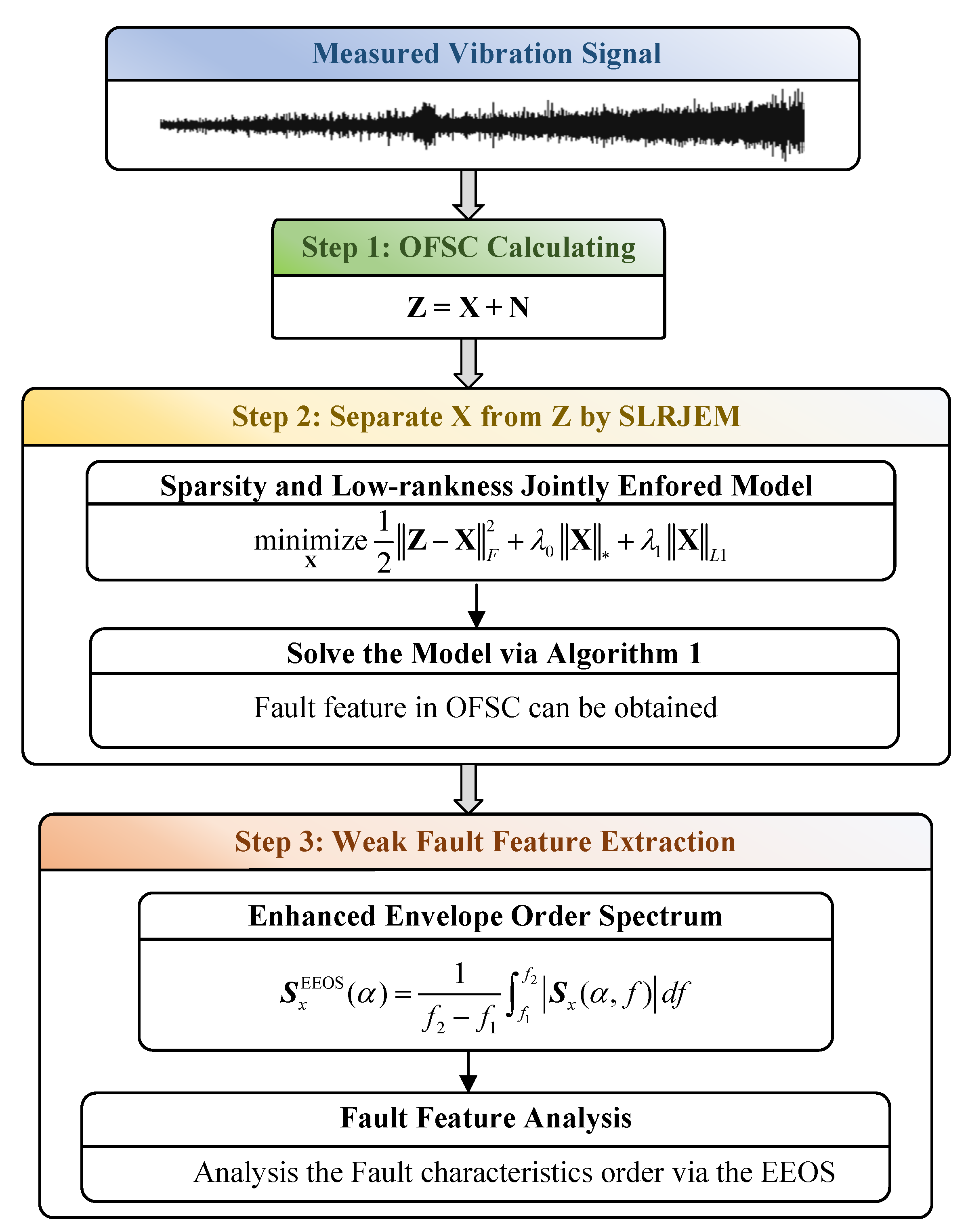
3.3. Process of the Proposed Extraction Method of Rolling Bearing Fault Feature

Figure 2 depicts the flowchart based on all of the preceding analyses. The OFSC of the measured vibration signal is firstly calculated. Then, the obtained OFSC is constrained as jointly sparse and low-rank and the derived algorithm is used to detect the time-varying faulty characteristic. Finally, the EEOS is computed to further enhance the fault feature in OFSC and the fault characteristic order can be further analyzed. The detailed process is:
  • Step 1: Resample the obtained vibration measurement into the angular domain and calculate the OFSC via Equation (4).
  • Step 2: Separate the fault feature X from the obtained OFSC Z via the proposed algorithm. The obtained OFSC is constrained as jointly sparse and low-rank, which is explained in Section 3.1. The derived algorithm in Section 3.2 named ADMM-SLRJEM is applied to separate the time-varying fault feature in the obtained OFSC.
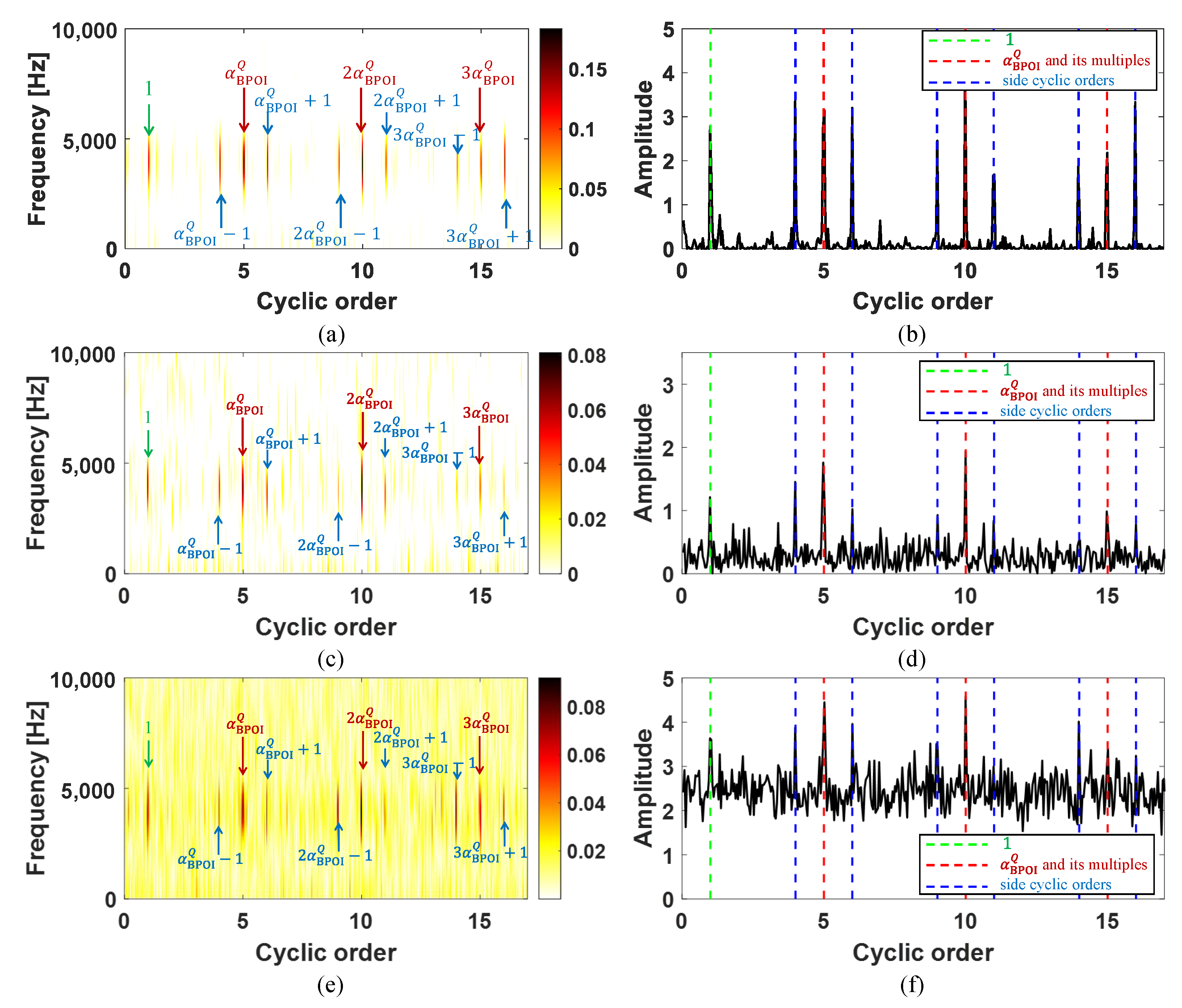
  • Step 3: Calculate the EEOS according to Equation (5) to further enhance the separated fault feature in OFSC. Then, the enhanced fault feature can be more obvious for fault diagnosis of rolling bearing with variable speed.
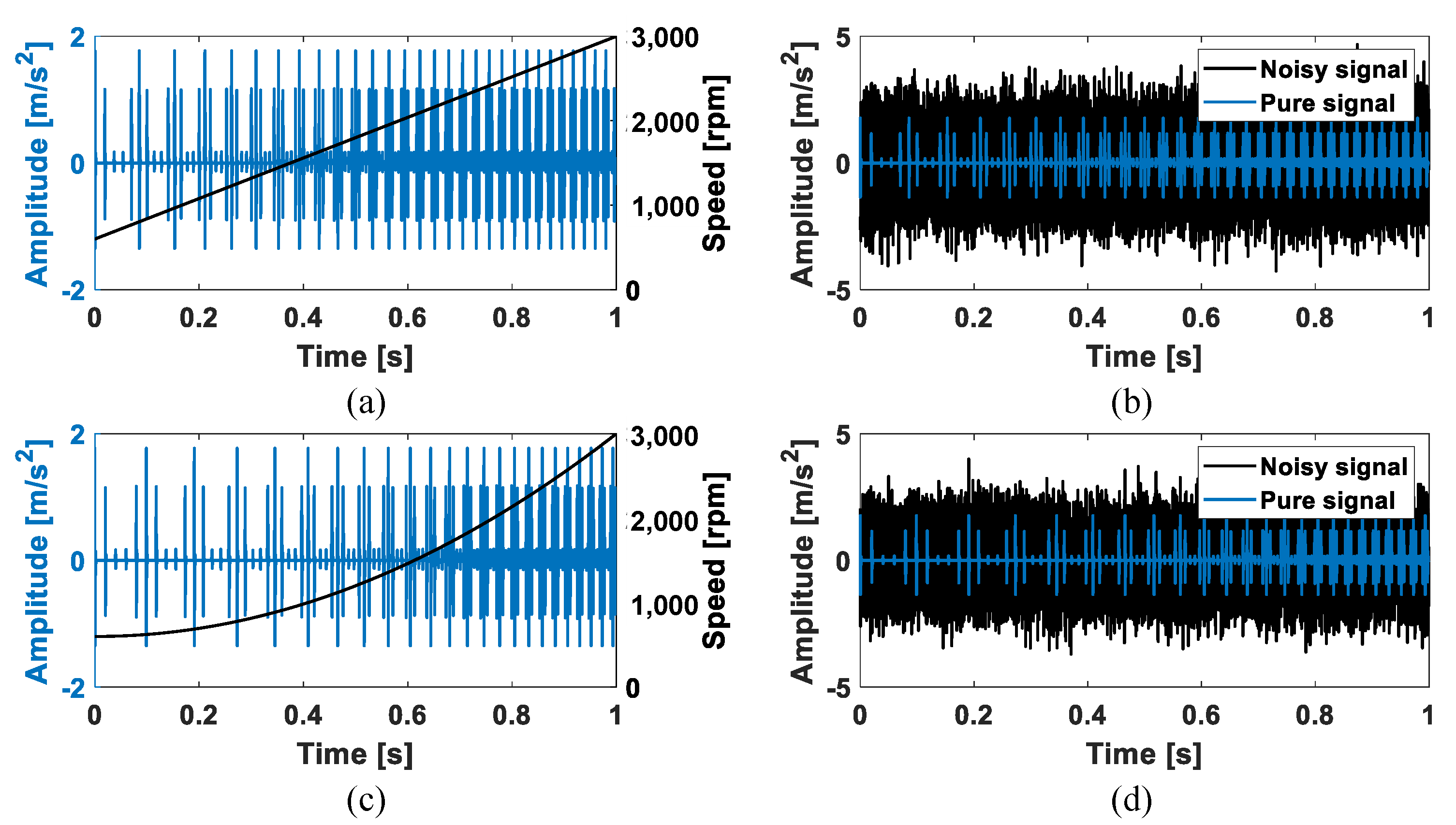
4. Simulation Study

In this section, several cases are simulated to confirm the performance of the proposed method. Firstly, three parameters λ 0 , λ 1 and ρ of the Algorithm 1 should be determined. The parameters λ 0 , λ 1 0 , 1 are related to the ratio of sparse and low-rank component. The more sparse and low-rank X is, the larger λ 0 and λ 1 are. The parameter ρ > 1 is related to the convergence speed and guarantee convergence, which has little impact on the extraction performance. Thus, λ 0 = 0.29 , λ 1 = 0.2 and ρ = 1.5 is adopted in this paper to achieve a better performance and proper speed for fault feature extraction in OFSC. The simulations in this section are carried out by MATLAB R2019b on Intel(R) Core(TM) i7-7700 CPU @ 3.60 GHz system with 16 GB-RAM. Note that there are few relevant studies focusing on the fault feature extraction in the cyclic order-frequency domain. Inspired by refs. [21,25] in the time-frequency domain, the proposed method is compared with methods imposing the single sparsity constraint and single low-rankness constraint on noisy OFSCs. Then, the outer and inner race fault (following the Equations (6) and (7)) is simulated in this section as two specific cases.

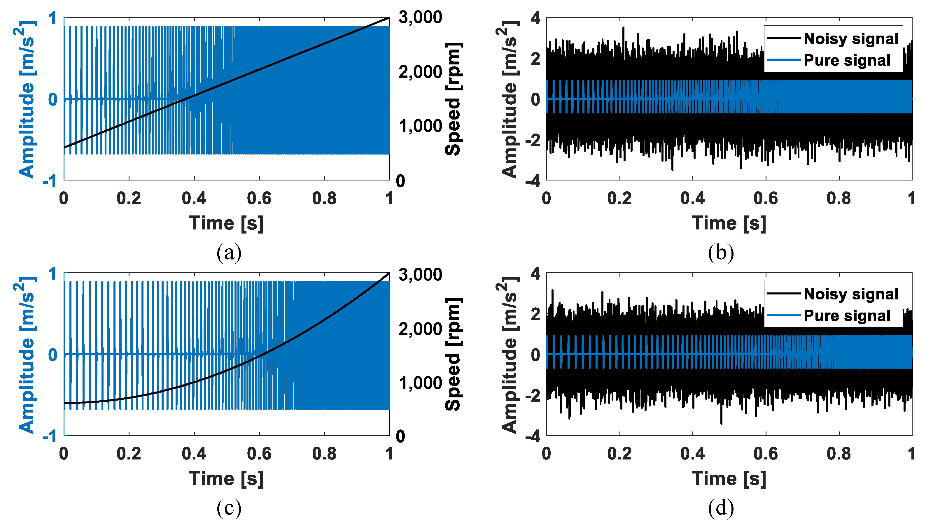
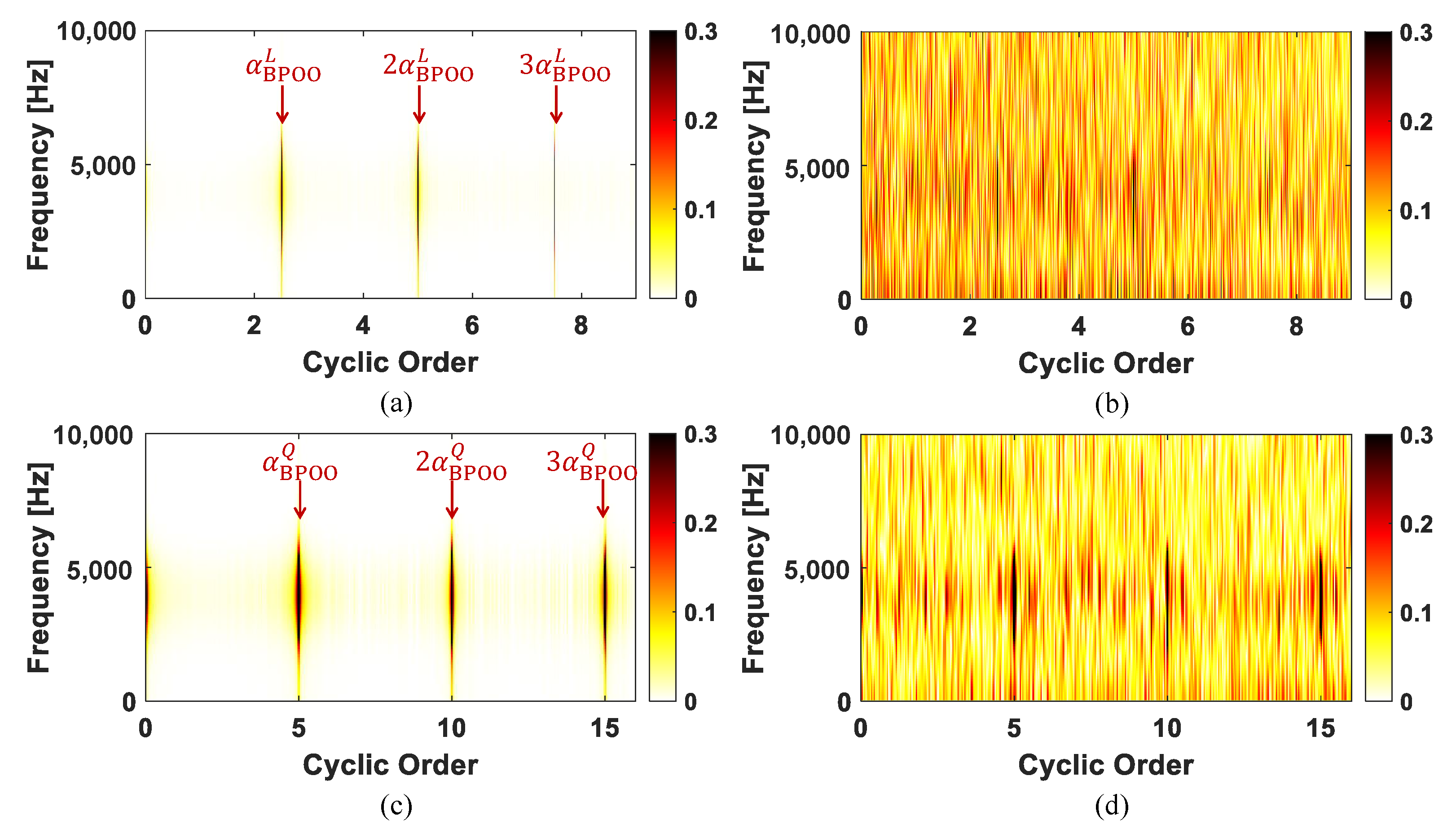
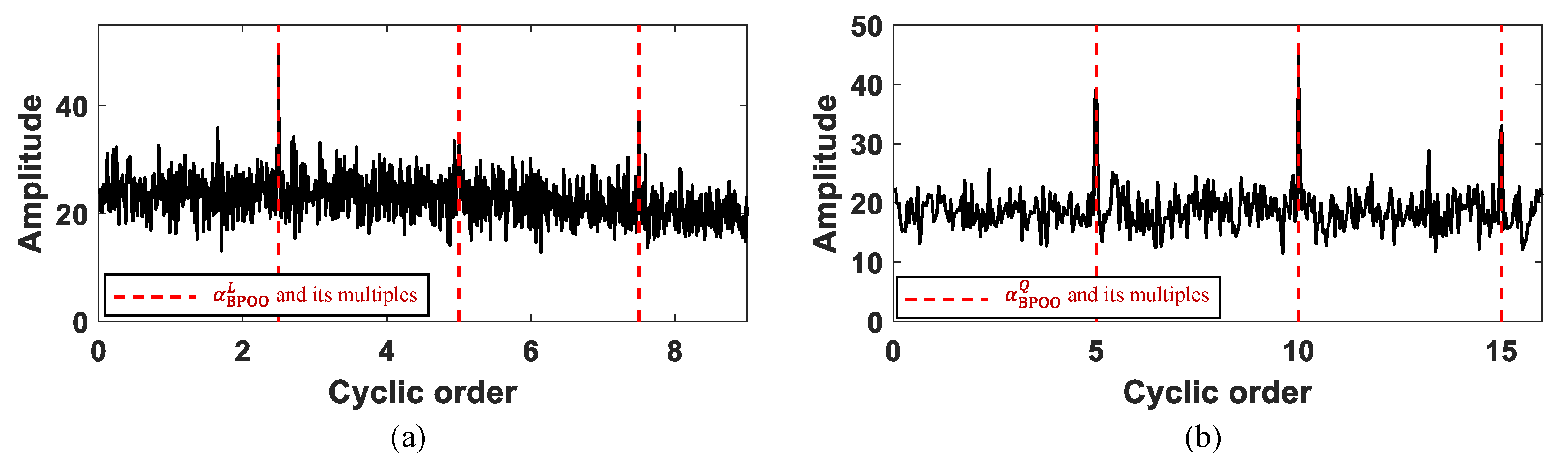
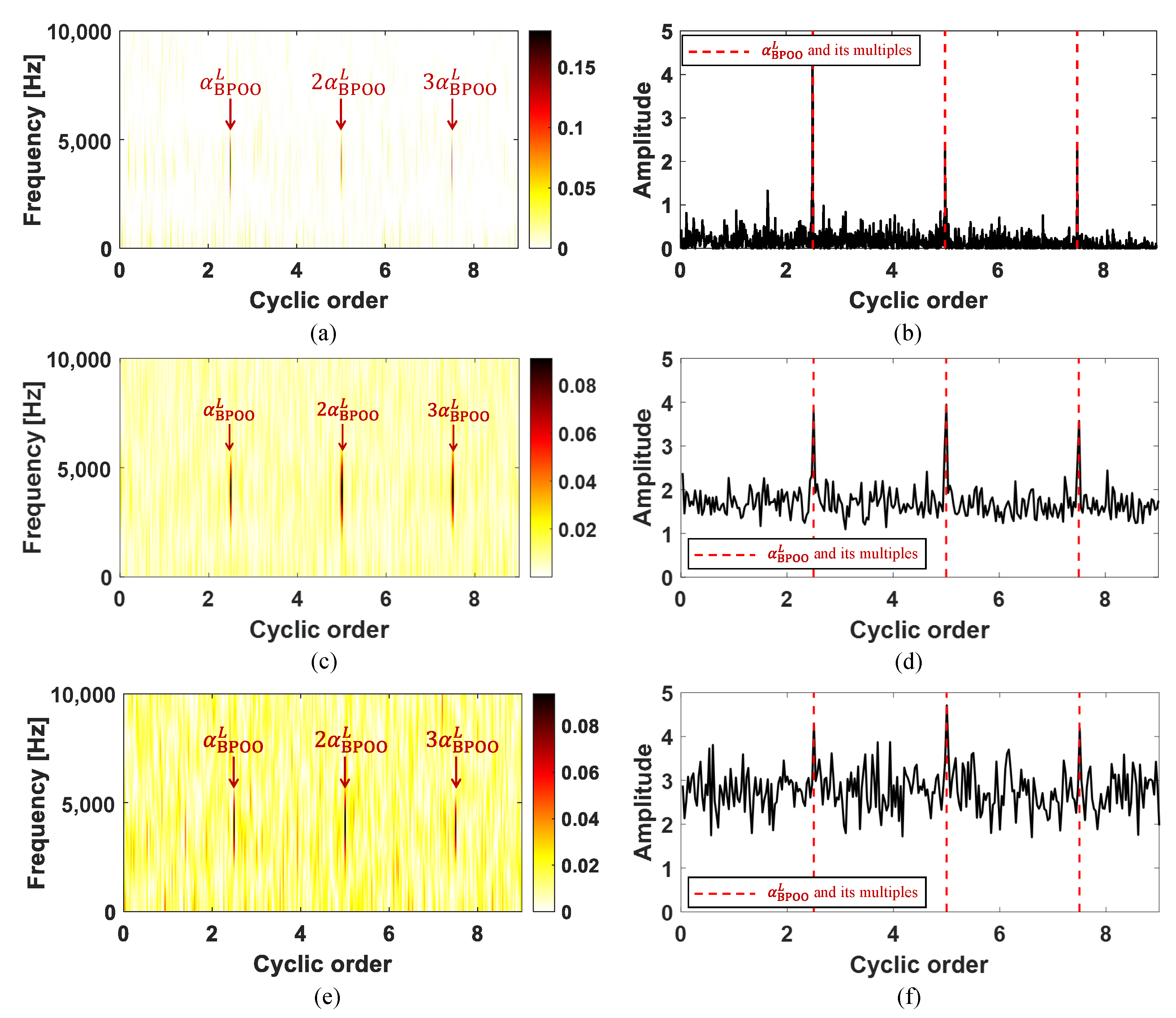
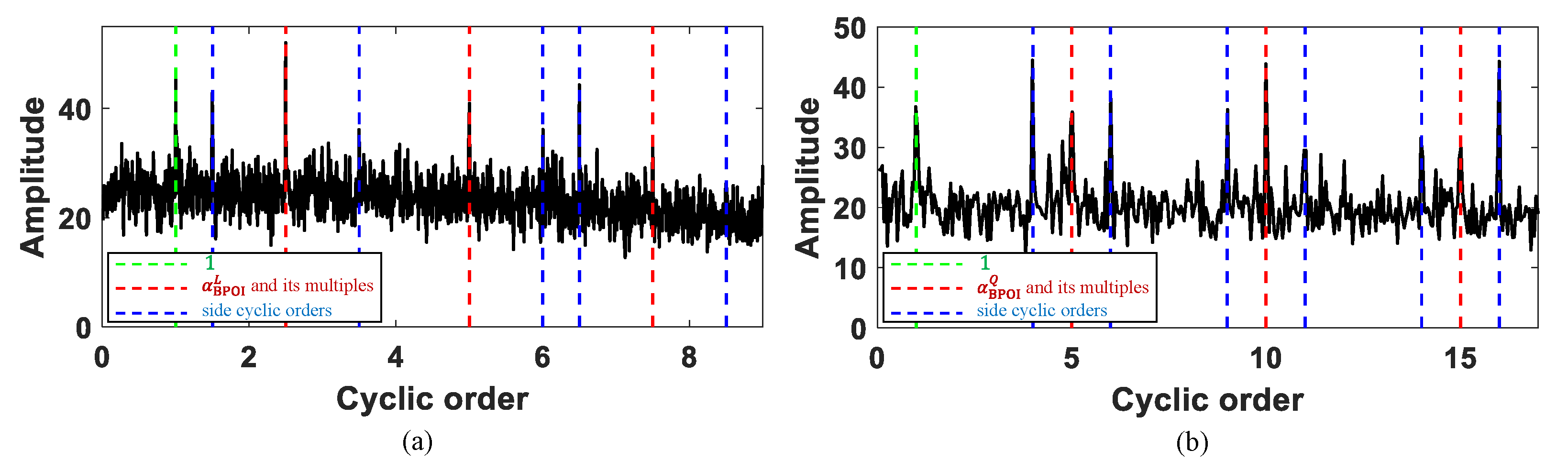
4.1. Case 1: Outer Race Fault

Two rotation speeds with linear function ( 40 t + 10 ) and quadratic function ( 40 t 2 + 10 ) are used with the ball-pass-order on the outer race (BPOO) of fault feature cyclic orders α BPOO L = 2.5 and α BPOO Q = 5 respectively are studied in this case. Other parameters are arranged as follows: the sampling frequency f s = 51,200 Hz, the sampling length N = 51,200 (a signal with one second), the resonance frequency f resonance = 4000 Hz and coefficient of resonance damping attenuation β = 2000 . The intervals between two transient impulses are decreasing with the increasing speed, which can be founded in Figure 3a,c. The Gaussian white noise (SNR = −16 dB) is added in simulated signals, which can be seen that the fault transient impulses are covered by the strong background noise (seen in Figure 3b,d).
Then, OFSC is computed to transfer the time-domain signal into the cyclic order-frequency domain. The time costs of the three methods are listed in Table 1, which can be seen that the computation burdens are similar. The OFSCs of the two simulated signals are shown in Figure 4. The fault cyclic orders (fault feature) can be found in the OFSCs of the pure transient impulses clearly. However, the strong background noise almost completely covers the fault feature as shown in Figure 4b,d. Then, the EEOSs of the two noisy OFSCs are tried to enhance the fault feature. Figure 5 shows that the fault cyclic orders are more pronounced compared with that in OFSCs, especially at the condition of α BPOO Q = 5 . The first order component at the condition of α BPOO L = 2.5 is obvious. However, its multipliers are still covered by the strong background noise, which needs to be effectively extracted.
Hereafter, the three methods are applied to the noisy OFSCs. The denoised results can be seen in Figure 6 and Figure 7. The fault feature can be effectively extracted with the proposed method for its joint sparsity and low-rankness inducing capability, as shown in Figure 6a and Figure 7a. The proposed method can effectively extract the outer race fault feature in OFSCs under variable speed conditions. As described in Section 3.1, the fault feature in OFSC is modeled as joint sparsity and low-rankness component. Thus, the components which mismatch the joint sparsity and low-rankness are unexpected (i.e., the strong background noise). The extraction result (seen in Figure 6c and Figure 7c) via single sparsity constraint can not extract the fault feature well, because the low-rankness of the fault feature in OFSC are not fully considered. Moreover, compared with the other two methods, the extraction results are the worst (seen in Figure 6e and Figure 7e). Similar to the noise component in the time-frequency domain, the noise component in the cyclic order-frequency domain also shows the low-rankness property. Thus, the noise component is also contained in the extraction result.
To make the fault cyclic order more clear, the EEOSs of the denoised OFSCs obtained by the proposed method are demonstrated in Figure 6b and Figure 7b. It can be seen that the noise near the fault cyclic order is significantly suppressed, which makes the fault feature more obvious. In the EEOSs obtained by the other two methods, the unseparated noise components in OFSC interfere the clear identification of α BPOO s, especially in Figure 6f and Figure 7d.
From all the above analyses, the proposed algorithm can effectively extract the outer race fault feature from strong background noise-contaminated OFSC with its superior sparsity and low-rankness inducing capability. The proposed method can achieve a better extraction performance than the other two methods in Case 1. Combined with EEOS, the fault cyclic order can be shown more obviously, which makes the determination of the fault type handier.

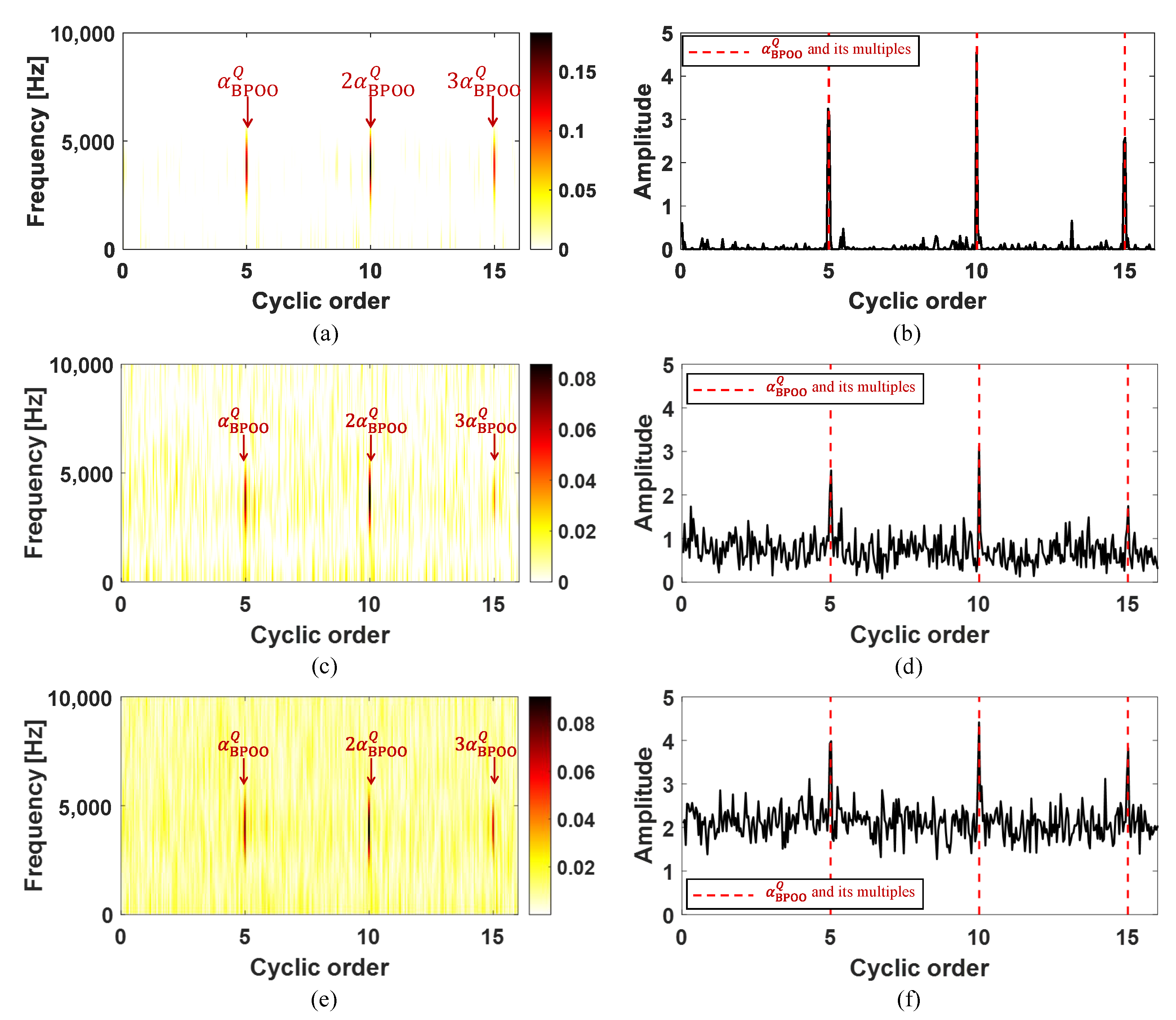
4.2. Case 2: Inner Race Fault

Similar to Section 4.1, the inner race fault is simulated to further confirm the proposed method. The ball-pass-order on the inner race (BPOI) of fault feature cyclic orders are set to α BPOI L = 2.5 and α BPOI Q = 5 respectively with the rotating shaft order 1. The rest of the parameter settings keep the same with Case 1. The simulated signals in Case 2 are displayed in Figure 8. One of the most obvious differences from Case 1 (Figure 8a,c) is that the transient impulses in Case 2 are modulated by the rotating frequency. The transient impulses are also covered by strong background noise from simulated signals.
Then, OFSCs in Case 2 are calculated and shown in Figure 9. The cyclic order one appears on the OFSCs in Case 2 as shown in Figure 9a,c, which indicates the shaft rotating order. The side cyclic order with the width two (BPOI ± 1 ) is also appeared and can be viewed as a characteristic of inner race fault. The OFSCs of the noisy signals are shown in Figure 9b,d, where the fault features are almost completely covered as well. The EEOSs of the noisy OFSCs in Case 2 are shown in Figure 10. The cyclic order of the inner race fault is relatively obvious on the single and double BPOI. The amplitude on triple BPOI tends to be covered by the noise. Moreover, the side cyclic orders are covered by the strong background noise, which are hard to identify.
The results after operating the three methods are shown in Figure 11 and Figure 12. At the quadratically changing speed condition ( α BPOI Q = 5 ), the proposed algorithm can effectively extract the fault feature (seen in Figure 12a, and the corresponding EEOS in Figure 12b shows it more clear. At the linearly changing speed condition ( α BPOI L = 2.5 ), the fault cyclic orders and their multipliers are effectively extracted. In comparison, the side cyclic orders are not obvious in Figure 11a. This may be due to the relatively lower amplitude on the side cyclic orders. From the EEOS of the denoised OFSC with linearly changing speed (seen in Figure 11b), the amplitude on the BPOI and its sides are larger than the components around them, which is more obvious. Compared with the other two methods, the noise components in OFSCs are not greatly eliminated due to the inadequate constraints, which make the time-varying fault features not clear enough to identify. Even according to EEOSs, the noise components interference the accurate judgment of the fault feature, especially in Figure 11d and Figure 12f.
From the above analysis, the proposed method is suitable for not only outer race fault but also inner race fault. The fault feature in OFSC can be effectively extracted via the proposed method. With the help of EEOS, the fault type can be further identified.

5. Experimental Validation

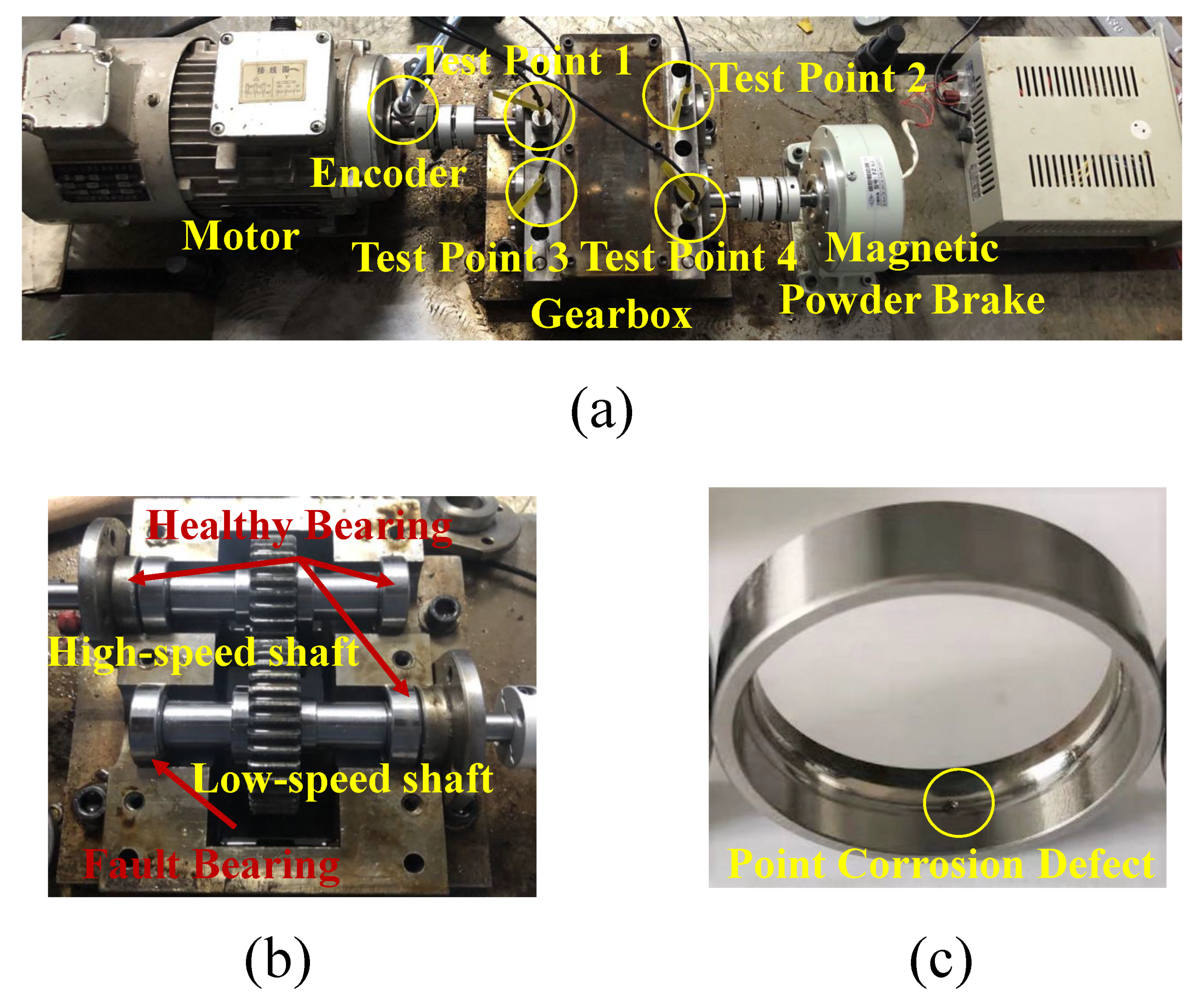
5.1. Experimental Layout

An outer-race fault experiment in a gearbox is carried out at Shanghai Jiao Tong University, of which the test layout is demonstrated in Figure 13. The shaft rotating frequency (SRF) is controlled by the inverter motor (YVP80M1) to generate the time-varying rotating speed signal. Four acceleration sensors (manufactured by Wuxi Houde Automation Meter Co., Ltd. with the type of HD-YD-221 and the sensitivity of 100 mV/g) are arranged on the test points as shown in Figure 13a. The sampling frequency is set as 51,200 Hz. There are two shafts in the gearbox, where three healthy bearings (corresponding to test points 1, 2 and 4) and one fault bearing (corresponding to test point 3) are illustrated as displayed in Figure 13a,b. Thus, the vibration signal measured on test point 3 is used for outer race fault feature extraction. Two standard spur gears with tooth numbers 28 and 39 respectively are meshed in the gearbox, which means that the measured signal on the measuring point will contain not only the rolling bearing fault component but also the gears meshing component.
In this experiment, the rolling bearing (type: 6203) with the outer race point corrosion defect (seen in Figure 13c) is processed by electric discharge machining (EDM). The tested rolling bearing parameters are listed in Table 2. Note that the α BPOO in this experiment can be calculated as
α BPOO = n 2 1 d D cos θ ,
where n is number of rolling balls, θ is the contact angle, d and D denote the pitch diameter and rolling element diameter respectively.

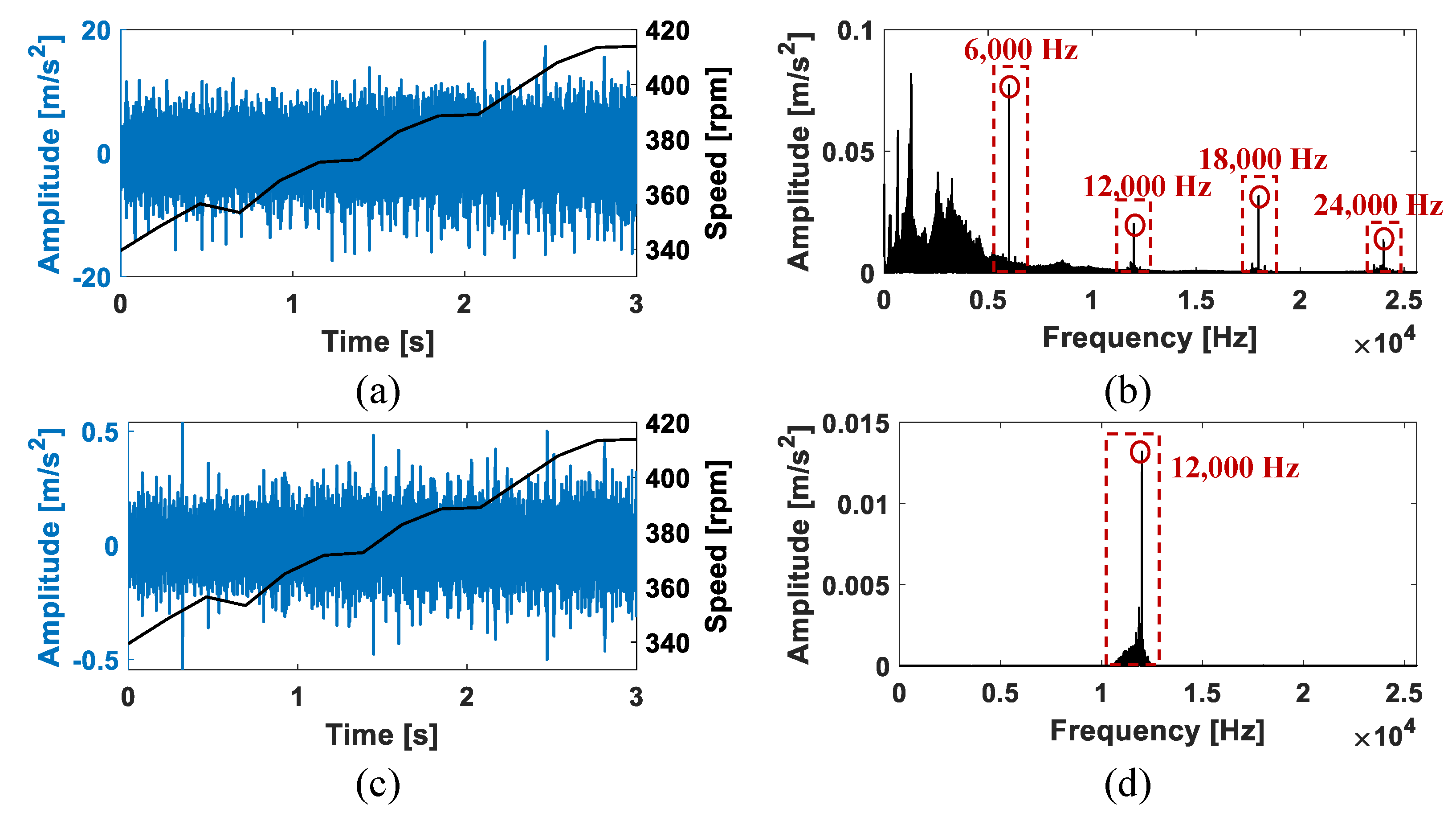
5.2. Data Preprocessing

As mentioned in Section 5.1, the measurement in this experiment contains the gear meshing component, which may have a great impact on the result of the proposed method. Therefore, the band-pass filtering should be carried out for the resonance frequency band. Figure 14b shows that the components of the gears meshing are focused on the lower frequencies and the centers of the resonance frequency band can be chosen as 6000 Hz, 12,000 Hz, 18,000 Hz and 24,000 Hz. In this paper, the filter band is set as [12,000 − 1000, 12,000 + 100] Hz. The filtered signal can be seen in Figure 14c. The impulses generated by the outer race fault are relatively clear compared with that unfiltered (seen in Figure 14a). The spectrum of the filtered signal is displayed in Figure 14d, which turns out the feasibility of the filtering. Then, the filtered signal with fewer gear meshing components can be used for fault feature extraction.

5.3. Extraction Results of the Outer Race Fault

In this subsection, the filtered signal is used for the outer race fault feature extraction. Figure 15a shows that the OFSC of the filtered signal can remain not to identify the BPOO, which is covered by the strong noise. The EEOS of the filtered signal’s OFSC is displayed in Figure 15b. The α BPOO and 2 α BPOO is clear, while 3 α BPOO covered by the noise is hard to identify. The OFSC and its EEOS of the proposed method are displayed in Figure 15c,d. Figure 15c illustrates that the fault feature in the OFSC is effectively extracted. Although the component of 3 α BPOO is weak overall, it is still stronger than the nearby components. This point of view can be also be confirmed in Figure 15d. Moreover, the noise in Figure 15c is also weakened by the joint sparsity and low-rankness constraint, which can make the target fault component more obvious. Compared with the other two methods, the noise components in OFSC are still greater than the denoised OFSC obtained by the joint sparsity and low-rankness constraint. The noise components in OFSC make the 3 α BPOO s hard to identify, which are covered by noise-generated cyclic orders nearby.
According to the experiment results, it turns out that the proposed method is capable of extracting the rolling bearing fault feature in OFSC. Moreover, the noise components in not only OFSC but also EEOS can be weakened, which is consistent with the results of simulation studies.

6. Conclusions

This paper proposes a weak fault feature extraction method for rolling bearings under variable speed circumstances. In the proposed method, the measured vibration signal is transferred into the (cyclic) order frequency domain and visualized by OFSC. Then, The joint sparsity and low-rankness of the fault feature in the OFSC is then exposed, which is utilized to extract the fault feature. Moreover, an algorithm is developed based on the ADMM framework to optimize the sparsity and low-rankness jointly enforced fault feature in the noisy OFSC. Finally, using EEOS, the fault feature of the rolling bearing is improved and the fault type can be more easily justified. In the simulation study, the proposed method can extract the fault feature under the strong background noise with SNR = −16 dB. In addition, an experimental case is carried out to validate the practicality of the proposed method. It shows that the proposed method can effectively extract the rolling bearing fault feature under variable speed conditions in a complex gearing system. However, there are some shortages of the proposed model and the algorithm needs to be further improved. For example, the adaptive selection of parameters λ 0 and λ 1 is still worth studying.

Author Contributions

Conceptualization, R.W., L.Y. and X.H.; methodology, C.Z.; software, C.Z., L.Y. and H.F.; validation, R.W. and C.Z.; formal analysis, R.W., C.Z. and H.F.; resouces, L.Y.; data curation, R.W.; writing—original draft preparation, C.Z.; writing—review and editing, R.W., L.Y. and H.F.; project administration, L.Y. and X.H.; funding acquisition, R.W. and L.Y. All authors have read and agreed to the published version of the manuscript.

Funding

This research was funded by the National Natural Science Foundation of China grant numbers 51505277 and 12074254, National Key Research and Development Program of China grant number 2019YFB2004600, Natural Science Foundation of Shanghai grant number 21ZR1434100. This research was also sponsored by the Oceanic Interdisciplinary Program of Shanghai Jiao Tong University project number SL2021MS009 and Open Fund of Laboratory of Vibration, Shock and Noise, Shanghai Jiao Tong University project number VSN202101.

Institutional Review Board Statement

Not applicable.

Informed Consent Statement

Not applicable.

Data Availability Statement

Not applicable.

Acknowledgments

The authors would like to appreciate Jin Chen (Shanghai Jiao Tong University) for providing experimental data. At the same time, the author would like to thank Junwu Zhang and Longjing Yu (Shanghai Maritime University) for their proof reading.

Conflicts of Interest

The authors declare no conflict of interest.

Abbreviations

The following abbreviations are used in this manuscript:
OFSCOrder-frequency spectral correlation
LRJEMLow-rankness jointly enforced model
ADMMAlternating direction method of multipliers
STFTShort-time Fourier transform
EESEnhanced envelope spectrum
EEOSEnhanced envelope order spectrum
FCFFault characteristic frequency
TFATime-frequency analysis
RPCARobust principal component analysis
SNRSignal-to-noise ratio
CNSCyclic non-stationary
AT-CSAngle-time cyclostationary
ATCFAngle-time autocorrelation function
SCSpectral correlation
SVDsingular value decomposition
SRFShaft rotating frequency

Appendix A. The Detailed Process to Obtain Equation (15) from Equation (12)

X ( k + 1 ) = arg min X ( k ) 1 2 Z X ( k ) F 2 + ρ 2 X ( k ) Y ( k ) + D ( k ) F 2 + λ 1 X ( k ) L 1 = arg min X ( k ) 1 2 Z X ( k ) F 2 + ρ 2 Y ( k ) + D ( k ) X ( k ) F 2 + λ 1 X ( k ) L 1 = arg min X ( k ) 1 2 Z X ( k ) F 2 + 1 2 ρ Y ( k ) + D ( k ) ρ X ( k ) F 2 + λ 1 X ( k ) L 1 = arg min X ( k ) 1 2 Z X ( k ) ρ X ( k ) + ρ Y ( k ) + D ( k ) F 2 + λ 1 X ( k ) L 1 = arg min X ( k ) 1 2 Z + ρ Y ( k ) + D ( k ) ( 1 + ρ ) X ( k ) F 2 + λ 1 X ( k ) L 1 = arg min X ( k ) 1 + ρ 2 1 1 + ρ Z + ρ Y ( k ) + D ( k ) X ( k ) F 2 + λ 1 X ( k ) L 1 = arg min X ( k ) 1 2 1 1 + ρ Z + ρ Y ( k ) + D ( k ) X ( k ) F 2 + λ 1 1 + ρ X ( k ) L 1 .

References

  1. Yang, B.; Liu, R.; Chen, X. Fault diagnosis for a wind turbine generator bearing via sparse representation and shift-invariant K-SVD. IEEE Trans. Ind. Inf. 2017, 13, 1321–1331. [Google Scholar] [CrossRef]
  2. Jiang, X.; Cheng, X.; Shi, J.; Huang, W.; Shen, C.; Zhu, Z. A new l0-norm embedded MED method for roller element bearing fault diagnosis at early stage of damage. Measurement 2018, 127, 414–424. [Google Scholar] [CrossRef]
  3. Jin, Y.; Qin, C.; Huang, Y.; Liu, C. Actual bearing compound fault diagnosis based on active learning and decoupling attentional residual network. Measurement 2021, 173, 108500. [Google Scholar] [CrossRef]
  4. Randall, R.B.; Antoni, J. Rolling element bearing diagnostics—A tutorial. Mech. Syst. Signal Process. 2011, 25, 485–520. [Google Scholar] [CrossRef]
  5. Xie, Z.; Zhu, W. An investigation on the lubrication characteristics of floating ring bearing with consideration of multi-coupling factors. Mech. Syst. Signal Process. 2022, 162, 108086. [Google Scholar] [CrossRef]
  6. Zmarzły, P. Multi-Dimensional Mathematical Wear Models of Vibration Generated by Rolling Ball Bearings Made of AISI 52100 Bearing Steel. Materials 2020, 13, 5440. [Google Scholar] [CrossRef]
  7. Tang, G.; Wang, X.; He, Y. Diagnosis of compound faults of rolling bearings through adaptive maximum correlated kurtosis deconvolution. J. Mech. Sci.Technol. 2016, 30, 43–54. [Google Scholar] [CrossRef]
  8. Arpaia, P.; Cesaro, U.; Chadli, M.; Coppier, H.; De Vito, L.; Esposito, A.; Gargiulo, F.; Pezzetti, M. Fault detection on fluid machinery using Hidden Markov Models. Measurement 2020, 151, 107–126. [Google Scholar] [CrossRef]
  9. Zhu, H.; He, Z.; Wei, J.; Wang, J.; Zhou, H. Bearing fault feature extraction and fault diagnosis method based on feature fusion. Sensors 2021, 21, 2524. [Google Scholar] [CrossRef]
  10. Qiao, W.; Lu, D. A Survey on Wind Turbine Condition Monitoring and Fault Diagnosis—Part II: Signals and Signal Processing Methods. IEEE Trans. Ind. Electron. 2015, 62, 6546–6557. [Google Scholar] [CrossRef]
  11. Borghesani, P.; Ricci, R.; Chatterton, S.; Pennacchi, P. A new procedure for using envelope analysis for rolling element bearing diagnostics in variable operating conditions. Mech. Syst. Signal Process. 2013, 38, 23–35. [Google Scholar] [CrossRef]
  12. Ding, C.; Zhao, M.; Lin, J.; Jiao, J. Multi-objective iterative optimization algorithm based optimal wavelet filter selection for multi-fault diagnosis of rolling element bearings. ISA Trans. 2019, 88, 199–215. [Google Scholar] [CrossRef] [PubMed]
  13. Antoni, J.; Randall, R.B. The spectral kurtosis: Application to the vibratory surveillance and diagnostics of rotating machines. Mech.Syst. Signal Process. 2006, 20, 308–331. [Google Scholar] [CrossRef]
  14. Antoni, J. The spectral kurtosis: A useful tool for characterizing non-stationary signals. Mech. Syst. Signal Process. 2006, 20, 282–307. [Google Scholar] [CrossRef]
  15. Jiang, X.; Shen, C.; Shi, J.; Zhu, Z. Initial center frequency-guided VMD for fault diagnosis of rotating machines. J. Sound Vib. 2018, 435, 36–57. [Google Scholar] [CrossRef]
  16. Li, H.; Liu, T.; Wu, X.; Li, S. Research on test bench bearing fault diagnosis of improved EEMD based on improved adaptive resonanceance technology. Measurement 2019, 185, 109986. [Google Scholar] [CrossRef]
  17. Li, H.; Liu, T.; Wu, X.; Chen, Q. Application of EEMD and improved frequency band entropy in bearing fault feature extraction. ISA Trans. 2019, 88, 170–185. [Google Scholar] [CrossRef]
  18. Li, H.; Liu, T.; Wu, X.; Chen, Q. Research on bearing fault feature extraction based on singular value decomposition and optimized frequency band entropy. Mech. Syst. Signal Process. 2019, 118, 477–502. [Google Scholar] [CrossRef]
  19. Hou, F.; Selesnick, I.W.; Chen, J.; Dong, G. Fault diagnosis for rolling bearings under unknown time-varying speed conditions with sparse representation. J. Sound Vib. 2021, 494, 115854. [Google Scholar] [CrossRef]
  20. Wang, R.; Fang, H.; Yu, L.; Chen, J. Sparse and low-rank decomposition of the time–frequency representation for bearing fault diagnosis under variable speed conditions. ISA Trans. 2021. [Google Scholar] [CrossRef]
  21. Yang, H.; Mathew, J.; Ma, L. Fault diagnosis of rolling element bearings using basis pursuit. Mech. Syst. Signal Process. 2005, 19, 341–356. [Google Scholar] [CrossRef]
  22. Huang, H.; Baddour, N.; Liang, M. Bearing fault diagnosis under unknown time-varying rotational speed conditions via multiple time-frequency curve extraction. J. Sound Vib. 2018, 414, 43–60. [Google Scholar] [CrossRef]
  23. Yu, L.; Dai, W.; Huang, S.; Jiang, W. Sparse Time–Frequency Representation for the Transient Signal Based on Low-Rank and Sparse Decomposition. J. Acoust. 2019, 1, e190003. [Google Scholar]
  24. Wright, J.; Ganesh, A.; Rao, S.; Ma, Y. Robust principal component analysis: Exact recovery of corrupted low-rank matrices via convex optimization. arXiv 2009, arXiv:0905.0233v2. [Google Scholar]
  25. Du, Z.; Chen, X.; Zhang, H.; Yang, B.; Zhai, Z.; Yan, R. Weighted low-rank sparse model via nuclear norm minimization for bearing fault detection. J. Sound Vib. 2017, 400, 270–287. [Google Scholar] [CrossRef]
  26. Zhang, H.; Chen, X.; Zhang, X. A clustering low-rank approach for aero-enging bearing fault detection. In Proceedings of the 2019 IEEE International Instrumentation and Measurement Technology Conference, Auckland, New Zealand, 20–23 May 2019; pp. 1–6. [Google Scholar]
  27. Wang, B.; Liao, Y.; Ding, C.; Zhang, X. Periodical sparse low-rank matrix estimation algorithm for fault detection of rolling bearings. ISA Trans. 2020, 101, 366–378. [Google Scholar] [CrossRef]
  28. Wang, B.; Liao, Y.; Duan, R.; Zhang, X. Sparse Low-Rank Based Signal Analysis Method for Bearing Fault Feature Extraction. Appl. Sci. 2021, 10, 2358. [Google Scholar] [CrossRef] [Green Version]
  29. Parekh, A.; Selesnick, I.W. Improved sparse low-rank matrix estimation. Signal Process. 2017, 139, 62–69. [Google Scholar] [CrossRef] [Green Version]
  30. Feng, Z.; Liang, M.; Chu, F. Recent advances in time-frequency analysis methods for machinery fault diagnosis: A review with application examples. Mech. Syst. Signal Process. 2013, 38, 165–205. [Google Scholar] [CrossRef]
  31. Borghesani, P.; Pennacchi, P.; Randall, R.B. Order tracking for discrete-random separation in variable speed conditions. Mech. Syst. Signal Process. 2012, 30, 1–22. [Google Scholar] [CrossRef]
  32. Hou, B.; Wang, Y.; Tang, B.; Qin, Y.; Chen, Y. A tacholess order tracking method for wind turbine planetary gearbox fault detection. Meas. J. Int. Meas. Confed. 2019, 138, 266–277. [Google Scholar] [CrossRef]
  33. Abboud, D.; Antoni, J.; Eltabach, M.; Sieg, Z.S. Anglentime cyclostationarity for the analysis of rolling element bearing vibrations. Measurement 2015, 75, 29–39. [Google Scholar] [CrossRef]
  34. Abboud, D.; Antoni, J.; Leclere, Q. Spectral matrix completion by Cyclic Projection and application to sound source reconstruction from non-synchronous measurements. J. Sound Vib. 2016, 372, 31–49. [Google Scholar]
  35. Abboud, D.; Antoni, J. Order-frequency analysis of machine signals. Mech. Syst. Signal Process. 2017, 87, 229–258. [Google Scholar] [CrossRef]
  36. Jiao, Y.; Jin, Q.; Lu, X.; Wang, W. Alternating direction method of multipliers for linear inverse problems. SIAM J. Numer. Anal. 2016, 54, 2114–2137. [Google Scholar] [CrossRef]
  37. Yu, H.; Neely, M.J. A Simple Parallel Algorithm with an O(1/t) Convergence Rate for General Convex Programs. arXiv 2015, arXiv:1512.08370v3. [Google Scholar] [CrossRef] [Green Version]
  38. Donoho, D.L. De-noising by soft-thresholding. IEEE Trans. Inf. Theory 1995, 41, 613–627. [Google Scholar] [CrossRef] [Green Version]
Figure 1. The faulty signal of rolling bearing with variable speed. (a) The signal and speed with the line in blue the signal waveform (adhering the left y-axis), the line in orange the shaft rotating speed (adhering the right y-axis); (b) the fault feature in the OFSC; (c) the normalized singular value of the fault feature in the OFSC.
Applsci 12 02449 g001
Figure 2. The flowchart of the proposed extraction method.
Applsci 12 02449 g002
Figure 3. The simulated signals in Case 1. (a) the transient impulses and rotation speed with linear function (line in blue: the signal waveform adhering the left y-axis and line in black: the shaft rotating speed adhering the right y-axis); (b) the noisy signal with linear function; (c) the transient impulses and rotation speed with quadratic function (line in blue: the signal waveform adhering the left y-axis and line in black: the shaft rotating speed adhering the right y-axis); (d) the noisy signal with quadratic function.
Applsci 12 02449 g003
Figure 4. The OFSCs of simulated signals in Case 1. (a) the OFSC of pure signal with linearly changing rotation speed; (b) the OFSC of noisy signal with linearly changing rotation speed; (c) the OFSC of pure signal with quadratically changing rotation speed; (d) the OFSC of noisy signal with quadratically changing rotation speed.
Applsci 12 02449 g004
Figure 5. The EEOSs of noisy OFSCs in Case 1. The dash lines in red indicate the corresponding BPOO and its multipliers. (a) the EEOS of noisy OFSC with linearly changing rotation speed; (b) the EEOS with noisy OFSC with quadratically changing rotation speed.
Applsci 12 02449 g005
Figure 6. The extraction results of Case 1 under the linearly changing rotation speed condition. The dash lines in red indicate the corresponding BPOO and its multipliers. (a) the denoised OFSC obtained by the proposed joint sparsity and low-rankness constraint; (b) the EEOS obtained by the proposed joint sparsity and low-rankness constraint; (c) the denoised OFSC obtained by single sparsity constraint; (d) the EEOS obtained by single sparsity constraint; (e) the denoised OFSC obtained by single low-rankness constraint; (f) the EEOS obtained by single low-rankness constraint.
Applsci 12 02449 g006
Figure 7. The extraction results of Case 1 under the quadratically changing rotation speed condition. The dash lines in red indicate the corresponding BPOO and its multipliers. (a) the denoised OFSC obtained by the proposed joint sparsity and low-rankness constraint; (b) the EEOS obtained by the proposed joint sparsity and low-rankness constraint; (c) the denoised OFSC obtained by single sparsity constraint; (d) the EEOS obtained by single sparsity constraint; (e) the denoised OFSC obtained by single low-rankness constraint; (f) the EEOS obtained by single low-rankness constraint.
Applsci 12 02449 g007
Figure 8. The simulated signals in Case 2. (a) the transient impulses and rotation speed with linear function (line in blue: the signal waveform adhering the left y-axis and line in black: the shaft rotating speed adhering the right y-axis); (b) the noisy signal with linear function; (c) the transient impulses and rotation speed with quadratic function (line in blue: the signal waveform adhering the left y-axis and line in black: the shaft rotating speed adhering the right y-axis); (d) the noisy signal with quadratic function.
Applsci 12 02449 g008
Figure 9. The OFSCs of simulated signals in Case 2. (a) the OFSC of pure signal with linearly changing rotation speed; (b) the OFSC of noisy signal with linearly changing rotation speed; (c) the OFSC of pure signal with quadratically changing rotation speed; (d) the OFSC of noisy signal with quadratically changing rotation speed.
Applsci 12 02449 g009
Figure 10. The EEOSs of noisy OFSCs in Case 2. The dash lines in green, red and blue indicate the shaft rotating cyclic order, corresponding BPOO and its multipliers and side cyclic orders. (a) the EEOS of noisy OFSC with linearly changing rotation speed; (b) the EEOS with noisy OFSC with quadratically changing rotation speed.
Applsci 12 02449 g010
Figure 11. The extraction results of Case 2 under the linearly changing rotation speed condition. The dash lines in green, red and blue indicate the shaft rotating cyclic order, corresponding BPOO and its multipliers and side cyclic orders. (a) the denoised OFSC obtained by the proposed joint sparsity and low-rankness constraint; (b) the EEOS obtained by the proposed joint sparsity and low-rankness constraint; (c) the denoised OFSC obtained by single sparsity constraint; (d) the EEOS obtained by single sparsity constraint; (e) the denoised OFSC obtained by single low-rankness constraint; (f) the EEOS obtained by single low-rankness constraint.
Applsci 12 02449 g011
Figure 12. The extraction results of Case 2 under the quadratically changing rotation speed condition. The dash lines in green, red and blue indicate the shaft rotating cyclic order, corresponding BPOO and its multipliers and side cyclic orders. (a) the denoised OFSC obtained by the proposed joint sparsity and low-rankness constraint; (b) the EEOS obtained by the proposed joint sparsity and low-rankness constraint; (c) the denoised OFSC obtained by single sparsity constraint; (d) the EEOS obtained by single sparsity constraint; (e) the denoised OFSC obtained by single low-rankness constraint; (f) the EEOS obtained by single low-rankness constraint.
Applsci 12 02449 g012
Figure 13. The layout of the experiment. (a) the experiment rig; (b) two shafts in the gearbox; (c) the point corrosion defect on the outer race.
Applsci 12 02449 g013
Figure 14. The time domain waveform and spectrum of the measured signal before and after band-pass filtering. (a) the time domain waveform and rotating speed before band-pass filtering (line in blue: the signal waveform adhering the left y-axis and line in black: the shaft rotating speed adhering the right y-axis); (b) the spectrum before band-pass filtering; (c) the time domain waveform and rotating speed after band-pass filtering (line in blue: the signal waveform adhering the left y-axis and line in black: the shaft rotating speed adhering the right y-axis); (d) the spectrum after band-pass filtering.
Applsci 12 02449 g014
Figure 15. The extraction results of experimental data. The dash lines in red indicate the corresponding BPOO and its multipliers. (a) the noisy OFSC; (b) the noisy EEOS; (c) the denoised OFSC obtained by the proposed joint sparsity and low-rankness constraint; (d) the EEOS obtained by the proposed joint sparsity and low-rankness constraint; (e) the denoised OFSC obtained by single sparsity constraint; (f) the EEOS obtained by single sparsity constraint; (g) the denoised OFSC obtained by single low-rankness constraint; (h) the EEOS obtained by single low-rankness constraint.
Applsci 12 02449 g015
Table 1. Time costs of the three methods.
ConstraintTime
Joint sparsity and low-rankness6.04 s
Single sparsity6.23 s
Single low-rankness6.11 s
Table 2. The parameters of the rolling bearing that is tested.
TypeRolling Balls NumberRolling Element DiameterPitch Diameter α BPOO
620386.747 mm28.5 mm3.05
Publisher’s Note: MDPI stays neutral with regard to jurisdictional claims in published maps and institutional affiliations.

