Dynamic Workpiece Modeling with Robotic Pick-Place Based on Stereo Vision Scanning Using Fast Point-Feature Histogram Algorithm

Abstract

In the era of rapid development in industry, an automatic production line is the fundamental and crucial mission for robotic pick-place. However, most production works for picking and placing workpieces are still manual operations in the stamping industry. Therefore, an intelligent system that is fully automatic with robotic pick-place instead of human labor needs to be developed. This study proposes a dynamic workpiece modeling integrated with a robotic arm based on two stereo vision scans using the fast point-feature histogram algorithm for the stamping industry. The point cloud models of workpieces are acquired by leveraging two depth cameras, type Azure Kinect Microsoft, after stereo calibration. The 6D poses of workpieces, including three translations and three rotations, can be estimated by applying algorithms for point cloud processing. After modeling the workpiece, a conveyor controlled by a microcontroller will deliver the dynamic workpiece to the robot. In order to accomplish this dynamic task, a formula related to the velocity of the conveyor and the moving speed of the robot is implemented. The average error of 6D pose information between our system and the practical measurement is lower than 7%. The performance of the proposed method and algorithm has been appraised on real experiments of a specified stamping workpiece.

1. Introduction

Under the trend of Industry 4.0, the concept of unmanned factories has dramatically emerged. All the governments over the world are also promoting smart manufacturing policies. It is expected that by developing unmanned smart factories to cope with the current shortage of labor, many manufacturers have introduced production lines combined with the robotic arm. Especially, in the metal forming industry, manual work in the current situation still plays an important role [1]. Hence, to improve production efficiency and reduce labor costs, as well as reduce the danger of human loss when working with the high-temperature workpiece in the hot-stamping process [2], it is required that the objects are first arranged and placed in a position, and then the robot arm is used to pick up and unload the materials to achieve the loading and unloading of the objects. The pre-work then is more troublesome. In order to fully achieve automation of new-generation smart factories, the combination of robotic arms and visual images has gradually become the current development trend. Handreg et al. [3] illustrate an idea to convert the current standard cold forming process of curved panels in the shipbuilding industry to computerized process control and quality examination using a conventional press, crane set up, and point cloud model based on a 3D vision system to monitor the production process successively. As a suggestion for our study to utilize three-dimensional images in the stamping industry, we have processed the point cloud to estimate the six-axis degree of freedom position and feature point information of hot-stamping workpieces. The latest modern Microsoft Azure Kinect camera [4], which is an application of the Time of Flight (ToF) principle [5], is the vision device used for this application to establish a 3D point cloud model in the scene. Later, the point cloud is leveraged to process the 3D point cloud data through a point-to-feature matching algorithm [6] to identify the stamping workpiece and its 6-DoF (6 degrees-of-freedom) position. The stamping workpieces in this study are placed on a conveyor to perform dynamic pick-and-place. Guo et al. [7] have a similar method of using a Kinect camera and a laser scanner to construct the point cloud and identify the position of the fruits, which were later used for harvesting. Compared to their research, a system with two depth cameras calibrated by stereo calibration in our study will generate both a target model point cloud and a reference model point cloud. Hence, the demand for a lower processing time as well as accuracy can be met. Moreover, setting up two cameras with two different viewing angles also allows the point cloud to fully model the object with just one scan. After the 6-DoF position of the workpieces is figured out, they will be transferred by the conveyor and the robot arm will pick them into the stamping die. Zheng et al. [8] stated that in a hot-stamping production line of high-strength steel, in order to evade oxidation and plasticity reduction when the temperature falls, the sheet metal has to be shifted from the furnace to the stamping die as quickly as possible. Therefore, they have proposed a method of synchronizing the motion of the feeding system. A description related to the velocity of the conveyor and the moving speed of the robot is executed for the purpose of dynamic transmission as our main goal of this study. After being placed into the machine, the system will trigger a signal for stamping to move and complete stamping. Finally, the system achieves the dynamic workpiece feeding process.

2. Research Methodology

The study uses ToF cameras to build a three-dimensional model and uses a pose estimation system to identify the stamping workpiece. The conveyor is used as a transmission system for delivering the workpiece to the robot gripping area. The workpiece 6D positions are automatically uploaded to the controller and execute intelligently dynamic grasping.

2.1. Experimental Devices and Setup

The hardware devices used in this study are a 6-axis robotic arm of Syntec 81R.6 Axis (Syntec, Taiwan). for gripping experiments and a depth camera of Microsoft Azure (Microsoft, Redmond, WA, USA) for object recognition. In addition, a stepper motor of model StepSyn 103H7126-0461 (Sanyo Denki, Japan) and a driver of model DRV8825 (Texas Instruments, Dallas, TX, USA) are used to control the conveyor system that utilizes a microprocessor of Arduino Mega 2560 (Arduino, Italy).

Figure 1 demonstrates the overall setup of the system. Under the conditions of the experiment, the room temperature was applied (15–25 °C). The distance from both cameras to the object is in the range of 0.5 to 0.85 m, which satisfied the requirement of the manufacturer (>0.5 m). A computer will be utilized as the main controller, which is connected to the microprocessor, two depth cameras, and also the robot arm. The scanning area will contain two cameras which are integrated into a fixed aluminum frame. After the system has identified the posture of the objects, the conveyor will transmit the workpiece for the robot to perform the dynamic gripping. The robot grasps the stamping workpiece with the pneumatic gripper. Afterward, the full cycle of automation will be finished when the robot feeds the workpiece to the stamping machine.

2.2. Point Cloud Contrustion and Pre-Processing

In order to achieve the dynamic feeding system, first, the point cloud which is later used for pose estimation will be constructed [9]. Two depth devices are utilized for generating the point cloud model. Afterward, some filters will be applied to the scene point cloud with the purpose of resulting in the input object’s model for the lateral program.

2.2.1. Stereo Calibration Principle

Two ToF depth cameras will generate two distinguished point clouds. Combining these two point clouds will create a point cloud with more details so the data for the location system will be more accurate. Calibration for combining two point clouds is performed using the stereo calibration principle [10]. Stereo calibration will help the study to find out the transformation matrix rotation, R, and translation, t, between two RGB cameras of the Azure Kinect.

Firstly, to use stereo calibration, the parameters of the transformation between an object in 3D space and the 2D image observed by the camera from visual information have to be determined. The pinhole camera model used to calibrate a camera is described in Figure 2.

Considering that $\mathit{P}\left(X,Y,Z\right)$ is the 3D world coordinates point of the object, the 3D coordinate of the same point in the camera frame, ${\mathit{P}}_{\mathit{c}\mathit{a}\mathit{m}}$, is:

$${\mathit{P}}_{\mathit{c}\mathit{a}\mathit{m}}=\left[\begin{array}{cc}\mathit{R}& \mathit{t}\end{array}\right]\mathit{P}$$

(1)

where $\mathit{R}$ is the 3 × 3 rotation matrix and $\mathit{t}$ is the 3 × 1 translation matrix. Let $\mathit{p}\left(x,y\right)$ be the position of the 3D point in the image coordinate, this will result in the 3D to 2D mapping; here, $\mathit{K}$ is the intrinsic matrix of the camera:

$$\mathit{p}=\mathit{K}\left[\begin{array}{cc}\mathit{R}& \mathit{t}\end{array}\right]\mathit{P}$$

(2)

The definition of the intrinsic matrix of the camera is as follows:

$$\mathit{K}=\left[\begin{array}{ccc}{f}_x& 0& c_x\\ 0& f_y& c_y\\ 0& 0& 1\end{array}\right]$$

(3)

where $f_x$ is the X-axis focal length and $f_y$ is the Y-axis focal length of the camera, and $\left(c_x,c_y\right)$ is the coordinate of the principal point.

The camera calibration’s purpose is to find out the intrinsic parameter, $\mathit{K}$ matrix, and extrinsic parameters, $\mathit{R}$ and $\mathit{t}$ matrices. The calculation uses linear algebra to find all the parameters. To achieve these parameters, multiple images of a checkerboard with a fixed square size will be taken and all the calibration patterns (the cross-point of the black/white consecutive squares) in each image will be found. These calibration patterns in the image correspond to some 3D points in the world. These point-to-point correspondences will be stored, and after that, the non-linear algorithm is used to solve the calibration parameters.

After the intrinsic matrices ${\mathit{K}}_{\mathbf{1}}$ and ${\mathit{K}}_{\mathbf{2}}$ of the two cameras are known, the next problem is figuring out the rotation, ${\mathit{R}}_{\mathbf{12}}$, and translation, ${\mathit{t}}_{\mathit{12}}$, between camera 1 and camera 2, which will contribute to finding point correspondences in the left and right image planes. The schematic diagram of the stereo calibration of the two cameras is described in Figure 3.

Let ${\mathit{p}}_{\mathit{1}}$ and ${\mathit{p}}_{\mathbf{2}}$ be a point in the camera 1 and camera 2 image coordinates respectively, which is the mapping of world coordinate $\mathit{P}$ in 3D space (Figure 3). The fundamental matrix $\mathit{F}$ is defined as a mapping from a point in an image plane to an epipolar line in the other image. Therefore, the following equation can be obtained:

$${\mathit{l}}_{\mathbf{2}}=\mathit{F}{\mathit{p}}_{\mathbf{1}}$$

(4)

The form of the fundamental matrix in terms of the two camera projection matrices: ${\mathit{M}}_{\mathbf{1}}$ and ${\mathit{M}}_{\mathbf{2}}$, may be derived algebraically. The ray that is back-projected from ${\mathit{p}}_{\mathbf{1}}$ by ${\mathit{M}}_{\mathbf{1}}$ is obtained by solving:

$${\mathit{M}}_{\mathbf{1}}\mathit{P}={\mathit{p}}_{\mathbf{1}}$$

(5)

The one-parameter family of solutions of Equation (5) is of the form given by:

$$\mathit{P}\left(\mathsf{\lambda }\right)={\mathit{M}}_{\mathbf{1}}^{-1}{\mathit{p}}_{\mathbf{1}}+\mathsf{\lambda }{\mathit{C}}_{\mathbf{1}}$$

(6)

where ${\mathit{M}}_{\mathbf{1}}^{-1}$ is the pseudo-inverse of ${\mathit{M}}_{\mathbf{1}}$, i.e., ${\mathit{M}}_{\mathbf{1}}{\mathit{M}}_{\mathbf{1}}^{-1}=\mathit{I}$, and ${\mathit{C}}_{\mathbf{1}}$ is the null vector, namely the camera 1 center, defined by ${\mathit{M}}_{\mathbf{1}}{\mathit{C}}_{\mathbf{1}}=\mathbf{0}$. The ray is parametrized by the scalar $\mathsf{\lambda }$.

Now consider two situations: when $\mathsf{\lambda }=0$ and $\mathsf{\lambda }=\infty$, Equation (6) becomes:

$$\begin{array}{l}\mathsf{\lambda }=0 \to \mathit{P}={\mathit{M}}_{\mathbf{1}}^{-1}{\mathit{p}}_{\mathbf{1}}\\ \mathsf{\lambda }=\infty \to \mathit{P}={\mathit{C}}_{\mathbf{1}}\end{array}$$

(7)

These two points in the above situations can be imaged by camera 2, with projection matrix ${\mathit{M}}_{\mathbf{2}}$ at ${\mathit{M}}_{\mathbf{2}}{\mathit{M}}_{\mathbf{1}}^{-\mathbf{1}}{\mathit{p}}_{\mathbf{1}}$ and ${\mathit{M}}_{\mathbf{2}}{\mathit{C}}_{\mathbf{1}}$ respectively, in the second view. The epipolar line is the line joining these two projected points:

$${\mathit{l}}_{\mathbf{2}}=\left({\mathit{M}}_{\mathbf{2}}{\mathit{C}}_{\mathbf{1}}\right)\times \left({\mathit{M}}_{\mathbf{2}}{\mathit{M}}_{\mathbf{1}}^{-\mathbf{1}}{\mathit{p}}_{\mathbf{1}}\right)$$

(8)

From Equations (4) and (8), we obtain:

$$\mathit{F}=\left({\mathit{M}}_{\mathbf{2}}{\mathit{C}}_{\mathbf{1}}\right)\times \left({\mathit{M}}_{\mathbf{2}}{\mathit{M}}_{\mathbf{1}}^{-\mathbf{1}}\right)$$

(9)

Now that the cameras are calibrated, let us assume that the world origin is at the camera 1 center:

$$\begin{gathered} {\mathit{M}}_{\mathbf{1}}={\mathit{K}}_{\mathbf{1}}\left[\begin{array}{cc}\mathit{I}& \mathbf{0}\end{array}\right] \\ {\mathit{M}}_{\mathbf{2}}={\mathit{K}}_{\mathbf{2}}\left[\begin{array}{cc}{\mathit{R}}_{\mathbf{12}}& {\mathit{t}}_{\mathbf{12}}\end{array}\right] \end{gathered}$$

(10)

Then,

$$\begin{gathered} {\mathit{M}}_{\mathbf{1}}^{-\mathbf{1}}=\left[\begin{array}{c}{\mathit{K}}_{\mathbf{1}}^{-\mathbf{1}}\\ {\mathbf{0}}^T\end{array}\right] \\ {\mathit{C}}_{\mathbf{1}}=\left[\begin{array}{c}\mathbf{0}\\ 1\end{array}\right] \end{gathered}$$

(11)

Therefore, substitute ${\mathit{M}}_{\mathbf{1}}$, ${\mathit{M}}_{\mathbf{2}}$, ${\mathit{M}}_{\mathbf{1}}^{-\mathbf{1}}$, and ${\mathit{C}}_{\mathbf{1}}$ to Equations (10) and (11), then Equation (9) becomes:

$$\begin{gathered} \mathit{F}=\left({\mathit{M}}_{\mathbf{2}}{\mathit{C}}_{\mathbf{1}}\right)\times \left({\mathit{M}}_{\mathbf{2}}{\mathit{M}}_{\mathbf{1}}^{-1}\right) \\ =\left\{{\mathit{K}}_{\mathbf{2}}\left[\begin{array}{cc}{\mathit{R}}_{\mathbf{12}}& {\mathit{t}}_{\mathbf{12}}\end{array}\right]\times \left[\begin{array}{c}\mathbf{0}\\ 1\end{array}\right]\right\}\times \left\{{\mathit{K}}_{\mathbf{2}}\left[\begin{array}{cc}{\mathit{R}}_{12}& {\mathit{t}}_{12}\end{array}\right]\times \left[\begin{array}{c}{\mathit{K}}_{\mathbf{1}}^{-\mathbf{1}}\\ {\mathbf{0}}^{\mathit{T}}\end{array}\right]\right\} \\ =\left({\mathit{K}}_{\mathbf{2}}{\mathit{t}}_{\mathbf{12}}\right)\times \left({\mathit{K}}_{\mathbf{2}}{\mathit{R}}_{\mathbf{12}}{\mathit{K}}_{\mathbf{1}}^{-\mathbf{1}}\right) \end{gathered}$$

(12)

Hence, the expression for $\mathit{F}=\left({\mathit{K}}_{\mathbf{2}}{\mathit{t}}_{\mathbf{12}}\right)\times \left({\mathit{K}}_{\mathbf{2}}{\mathit{R}}_{\mathbf{12}}{\mathit{K}}_{\mathbf{1}}^{-\mathbf{1}}\right)$ is purely in terms of ${\mathit{K}}_{\mathbf{1}}$, ${\mathit{K}}_{\mathbf{2}}$, ${\mathit{R}}_{\mathbf{12}}$, and ${\mathit{t}}_{\mathbf{12}}$. The correspondence relation between the two images is defined by the fundamental matrix, $\mathit{F}$, as:

$${\mathit{p}}_2^T\mathit{F}{\mathit{p}}_{\mathbf{1}}=0$$

(13)

Using the checkerboard to take multiple pictures and find the position in each calibration pattern, multiple sets of ${\mathit{p}}_{\mathbf{1}}$ and ${\mathit{p}}_{\mathbf{2}}$ will be calculated. Then, the fundamental matrix, $\mathit{F}$, can be solved according to Equation (13). Afterward, Equation (12) is used to find the rotation matrix, ${\mathit{R}}_{\mathbf{12}}$, and the translation matrix, ${\mathit{t}}_{\mathbf{12}}$, where the other parameters $\mathit{F}$, ${\mathit{K}}_{\mathbf{1}}$, and ${\mathit{K}}_{\mathbf{2}}$ are known.

2.2.2. Object Segmentation

After the scene point cloud has been created and processed by the pass-through filter, statistical outlier removal filter, and voxel grid filter to achieve the proper view of the region of interest, the object’s point cloud will be segmented from the scene point cloud by combining the random sample consensus (RANSAC) [11] and the Euclidean cluster extraction algorithms [12].

The RANSAC Algorithm 1 is a learning technique to estimate the parameters of a model by random sampling of inspected data. RANSAC utilizes the voting scheme to estimate the optimal appropriate result of a processing dataset in which data components carry both inliers and outliers. Data components in the dataset are used to determine one or multiple models. In this study, the RANSAC algorithm was utilized to determine the plane model, and the following will illustrate its pseudocode.

Algorithm 1 RANSAC algorithm to find plane model

Input: Point cloud and model estimation.

Output: Plane Model $M$, which was rated best amongst all iterations

While ($i\le maxIterations$) do

Sample $k$ points;

Estimate a plane model $M$;

Compute model inliers;

If ($M$ is better than $bestModel$) then

$M≔bestModel$;

$updateMaxIteration()$;

End if;

$i≔i+1$;

End while;

Return $bestModel$

The target workpiece is placed on a worktable. In order to extract the point cloud of the target object, a worktable plane is required to be removed from the scene. After inputting the point cloud data, the plane model is estimated by applying RANSAC; then, the plane inliers are eliminated from the input cloud data [13].

To achieve the object extraction, a method called clustering classification is applied. A simple and powerful data clustering approach in the Euclidean sense can be executed using an octree data structure. This algorithm will calculate the minimum distance between points and divide the point cloud data into clusters by setting the distance threshold. The cluster definition formula is as follows:

$$min\left|p_i-p_j\right|\ge d_{th}$$

(14)

where $p_i$ is the $i$ point cloud data, $p_j$ is the $j$ point cloud data, and $d_{th}$ is the distance threshold. The distance between points is searched through the Nearest Neighbor Search (NNS) in the K-Dimension Tree (KD-Tree) [14], and the Euclidean cluster extraction algorithm is defined as follows Algorithm 2.

Algorithm 2 Euclidean cluster extraction algorithm to extract the workpiece point cloud

Input: Point cloud data $P$.

Output: Point cloud clusters $C_i$

$C_i≔\varnothing$;//list of clusters

$Q≔\varnothing$;//list of checked points

While ($p_i\in P$) do

$p_i\to Q$;

While ($p_i\in Q$) do

If ($r_{p_k}<d_{th}$) then

$p_k\to P_k$;

End if;

While ($p_k\in P_k$)

If ($p_k$ has not been processed) then

$p_k\to Q$;

End if;

End while;

End while;

If (all points $p_i\in Q$ are processed) then

$C_i≔Q$;

$\mathrm{Q}≔\varnothing$;

End if;

End while

After processing through the above steps, the original point cloud model can be clustered, and according to the threshold value, the target object from the scene can be obtained to be input in the pose estimation program. Figure 4 will demonstrate the effect as well as the steps of object segmentation in this study.

2.3. Pose Estimation System Construction

The cluster from the previous section segmentation will be the input cloud of the pose estimation system. In addition, a reference point cloud of the subject also has to be saved into the database before performing position prediction. Firstly, feature points of the object will be estimated for further evaluation. Then, the matching methods between the target point cloud and reference point cloud will be carried out by comparing the features point values.

2.3.1. Feature Point Descriptor

This study uses the fast point-feature histograms (FPFH) [15] to estimate the feature point. FPFH is the optimization method of its predecessor—point feature histograms (PFH) [16]. PFH has the theoretical computational complexity of a point cloud $P$ with $N$ points, $O\left(N·k^2\right)$, where $k$ is the number of neighbors for each point $p$ in $P$. The FPFH overtakes the PFH in this aspect with the complexity of $O\left(N·k\right)$, while still retaining the advantage of the PFH [7].

The FPFH algorithm proceeds as follows: for each query point $p$ with its normal vector $n$, only the relation between the point itself and its neighbors, $p_k$ (the neighbors are chosen inside the sphere with the radius $r$), with the normal vector $n_k$ (not between all of its neighbors as in PFH), is computed. Define the $uwv$ frame (where $u=n_k, v=\left(p-p_k\right)\times u, w=u\times v$) and the computation of the angular variations $\alpha , \varphi , \theta$ (which is called the simplified point feature histogram—SPFH) of $n$ and $n_k$ as follows:

$$\left\{\begin{array}{c}\alpha =v·n_k\\ \varphi =\left(u·\left(p-p_k\right)\right)/p-p_k\\ \theta =\arctan \left(w·n_k,u·n_k\right)\end{array}\right.$$

(15)

Then, the final histogram of $p$ is weighted through re-determination of its k-neighbors and the previous SPFH values:

$$FPFH\left(p\right)=SPFH\left(p\right)+\frac{1}{k}{\displaystyle \sum }_{i=1}^k\frac{1}{w_{ki}}·SPFH\left(p_{ki}\right)$$

(16)

where the weight, $w_{ki}$, indicates the distance between point $p$ and the neighbor point $p_{ki}$. Figure 5 shows the effect area of the FPFH algorithm. In the figure, the query point $p$ only linked with its direct neighbors $p_k$ (inside the red-dashed circle). Each of the neighbors, $p_k$ (in the figure, they are displayed with different colors with their own circle of region), are linked with their own neighbors. The resulted histogram is weighted together with the histogram of the point $p$ to estimate the FPFH value. The gray connections marked with number 2 between the point $p$ and its neighbors together have a weight twice as large as other normal connections. The FPFH value of each query point $p$ will be analyzed in the next stage of the study.

2.3.2. Coarse Alignment Matching

Coarse alignment matching provides an initial prediction of the change between two point clouds by applying the sample consensus initial alignment (SAC-IA) algorithm [17]. In the SAC-IA algorithm, the target object point cloud’s feature descriptors are matched with the reference’s feature descriptors to obtain a rough pose estimation. The series of points that have almost identical FPFH values in the object as well as reference point cloud will be figured out and then the transformation matrix between these corresponding points is determined. The completion of the prevailing registration transformation of the point cloud with $n$ times iteration is evaluated by the Huber penalty function, ${\displaystyle \sum }_{i=1}^{n}H\left(l_i\right)$, which is calculated by the following equation:

$$H\left(l_i\right)=\left\{\begin{array}{cc}\frac{1}{2}{l}_i^2& if \Vert l_i\Vert <m_l\\ \frac{1}{2}{m}_l\left(2\Vert l_i\Vert -m_l\right)& if \Vert l_i\Vert >m_l\end{array}\right.$$

(17)

where $m_l$ is the threshold which is predetermined, and $l_i$ is the distance differences between after and before the transformation of each point.

2.3.3. Finish Alignment Matching

After the coarse alignment matching through the SAC-IA algorithm, the iterative closest point (ICP) algorithm was applied to optimize the prediction and obtain the final 6-DoF pose [18]. The reference point cloud and target point cloud which have been transformed by the SAC-IA algorithm are considered as the input data for the ICP algorithm. Then, the nearest corresponding point, $Q_i$, will be found inside the target point cloud, $Q,$ for each point, $P_i$, of the reference point cloud, $P$. The finishing point pairs are built up through the pair $P_i$-$Q_i$. The error of the ICP finish alignment is defined by the acquired error of Euclidean distance between corresponding point pairs $P_i$-$Q_i$ through the following formula:

$$d_k=\frac{1}{N}{\displaystyle \sum }_1^N\Vert Q_i-R{P}_i+T\Vert$$

(18)

where $d_k$ is the Euclidean distance, $N$ is the number of iterations, and $R$ and $t$ are the rotation and the translation matrix of the finish alignment, respectively.

2.4. Position Error Compensation of Robot Arm

The robot arm has errors when going to the specified position using the linear movement. This error happens due to the non-linearity of the positive sensitive detector (PSD). To solve this problem, a polynomial fitting algorithm is proposed [19]; however, the method will consider only the error of the XY plane. The Z-axis error will be ignored because, in the range of the study, the height of the object is not enough for the Z-axis error to affect the accuracy of the system.

Due to the different manufacturing processes, the size of the non-linear error of the PSD of each robot arm will be different. According to the different degree of the non-linearity of the PSD, the photosensitive surface of the PSD is usually artificially divided into Region A and Region B. Region A is the center area which has good linearity and a small measurement error; on the other hand, Region B is the margin area, where the non-linear error is large and the measurement error is also large.

According to the principle of the PSD, the non-linear error of the PSD in the $x$ and $y$ directions is relatively independent. There are error values in the $x$ and $y$ directions for the measured values of each point on the PSD photosensitive surface. Consider the error of each point to be $E_x\left(x_i,y_j\right)$ for the X-axis and $E_y\left(x_i,y_j\right)$ for the Y-axis. Equation (19) defines the error:

$$\begin{gathered} \Delta x=E_x\left(x_i,y_i\right)=x_i-x_{i0} \\ \Delta y=E_y\left(x_i,y_i\right)=y_j-y_{j0} \end{gathered}$$

(19)

where $x_i$ and $y_j$ are the final positions after correction for the robot arm, and $x_{i0}$ and $y_{j0}$ are the positions after calculation of the pose estimation system from Section 2.3. According to the non-linear characteristics, the third-degree polynomials are chosen for fitting:

$$\begin{gathered} E_x\left(x_i,y_j\right)=a_1{x}^3+b_1{y}^3+c_1{x}^{2}y+d_{1}x{y}^2+e_1{x}^2+f_1{y}^2+g_{1}xy+h_{1}x+i_{1}y+k_1 \\ {E}_y\left(x_i,y_j\right)=a_2{x}^3+b_2{y}^3+c_2{x}^{2}y+d_{2}x{y}^2+e_2{x}^2+f_2{y}^2+g_{2}xy+h_{2}x+i_{2}y+k_2 \end{gathered}$$

(20)

The polynomial fitting is mainly the calculation of its coefficients, using the measured n-set of position coordinates and calculating according to Equation (19). Substituting $\Delta x$ and $\Delta y$ into Equation (20) leads to the following sets of Equation (21):

$$\begin{gathered} A=\left[\begin{array}{cccccccccc}{x}_1^3& y_1^3& x_1^2{y}_1& x_1{y}_1^2& x_1^2& y_1^2& x_1{y}_1& x_1& y_1& 1\\ x_2^3& y_2^3& x_2^2{y}_2& x_2{y}_2^2& x_2^2& y_2^2& x_2{y}_2& x_2& y_2& 1\\ x_3^3& y_3^3& x_3^2{y}_3& x_3{y}_3^2& x_3^2& y_3^2& x_3{y}_3& x_3& y_3& 1\\ x_4^3& y_4^3& x_4^2{y}_4& x_4{y}_4^2& x_4^2& y_4^2& x_4{y}_4& x_4& y_4& 1\\ ⋮& ⋮& ⋮& ⋮& ⋮& ⋮& ⋮& ⋮& ⋮& ⋮\\ x_{n-1}^3& y_{n-1}^3& x_{n-1}^2{y}_{n-1}& x_{n-1}{y}_{n-1}^2& x_{n-1}^2& y_{n-1}^2& x_{n-1}{y}_{n-1}& x_{n-1}& y_{n-1}& 1\\ x_n^3& y_n^3& x_n^2{y}_n& x_n{y}_n^2& x_n^2& x_n^2& x_n{y}_n& x_n& y_n& 1\end{array}\right] \\ B=\left[\begin{array}{cc}\Delta x_1& \Delta y_1\\ \Delta x_2& \Delta y_2\\ \Delta x_3& \Delta y_3\\ \Delta x_4& \Delta y_4\\ ⋮& ⋮\\ \Delta x_{n-1}& \Delta y_{n-1}\\ \Delta x_n& \Delta y_n\end{array}\right];C=\left[\begin{array}{cc}{a}_1& a_2\\ b_1& b_2\\ c_1& c_2\\ d_1& d_2\\ e_1& e_2\\ f_1& f_2\\ g_1& g_2\\ h_1& h_2\\ i_1& i_2\\ k_1& k_2\end{array}\right] \end{gathered}$$

(21)

Then, the equation of $A\times C=B$ can be obtained using the least square method to solve the coefficient, as shown in Equation (22):

$$C={\left(A^{T}A\right)}^{-1}{A}^{T}B$$

(22)

After finding all the coefficients by using Equation (22), these coefficients are applied back into Equation (19) and the actual position after correction is obtained:

$$\begin{gathered} X_R=X_{out}-\Delta x \\ {Y}_R=Y_{out}-\Delta y \end{gathered}$$

(23)

where $X_R$ and $Y_R$ are the actual position for the robot, $X_{out}$ and $Y_{out}$ are the output measured values, and $\Delta x$ and $\Delta y$ are the coefficients calculated above.

2.5. Synchronization of Transmission Conveyor and Robot Arm

In order to accomplish the automation production line, we used a Syntec robot and a microcontroller-controlled conveyor to transfer the workpiece to the stamping die. Furthermore, for the dynamic transmission workpiece to take place successfully, a formula needs to be proposed to synchronize the movement of the robot and the conveyor.

First of all, the gripping position, $P_{gripping}$, needs to be recognized. To achieve the gripping pose, the point cloud of the object in the reference position has to be considered. The robot arm will be set to this position and its coordinates will be saved to the database for calculating the later position change of the object. After the pose estimation system figures out the relative position differences between the target point cloud and the reference point cloud, the gripping position of the target object, $P_{gripping}$, will be calculated as the sum of the reference position stored in the database, $P_{database}$, and the relative position, $P_{estimate}$. Equation (24) and Figure 6 describe the grab position of the target object.

$$P_{gripping}=P_{database}+P_{estimate}$$

(24)

Figure 7 depicts the home position of the robot, $P_{robot}$, and the scanning position of the conveyor, $P_{scan}$, to the gripping position, $P_{gripping}$. These positions, $P_{robot}$ and $P_{scan}$, need to be known in advance and pre-set in the database to synchronize the operation of the robot and the conveyor.

The travel time for the robot to move from the home position to the gripping position of the object, $t_{R\to G}$, is calculated as the distance between the robot’s initial position, $P_{robot}$, and the gripping position, $P_{gripping}$, divided by the feed rate of the robot in linear movement, $FL$. The following will demonstrate how to find $t_{R\to G}$:

$$t_{R\to G}=\frac{\left|P_{robot}-P_{gripping}\right|}{FL}$$

(25)

The time, $t_{S\to G}$, for the conveyor to move from the scan position to the gripping position is calculated by the distance of the scan position of the object, $P_{scan}$, to the gripping position, $P_{gripping}$, divided by the speed of the conveyor, $v_{conveyor}$. $t_{S\to G}$ will be expressed by:

$$t_{S\to G}=\frac{\left|P_{scan}-P_{gripping}\right|}{v_{conveyor}}$$

(26)

Travel times $t_{R\to G}$ and $t_{S\to G}$ have to be synchronized for the robot to successfully pick the workpiece while the conveyor is moving; therefore, $t_{R\to G}=t_{S\to G}$. Substitute into Equations (25) and (26), obtaining:

$$v_{conveyor}=\frac{FL\times \left|P_{scan}-P_{gripping}\right|}{\left|P_{robot}-P_{gripping}\right|}$$

(27)

Equation (27) indicates that the $v_{conveyor}$ will be the linear function of the feed rate of the robot in linear movement, $FL$.

3. Experimental Results

This study focuses on the pose estimation and the robot pick-place system. Consequently, results that need to be found first are from the experiment on how accurately the program can predict the position of the workpiece. Then, with the information conducted from the pose estimation system, robot pick-place experiments were performed and resulted in quantity visualization. Moreover, the robot error compensation results will be demonstrated to verify the nonlinear correction method and increase the success rate of dynamic pick-placing.

3.1. Experiment on the Accuracy of the Pose Estimation System

The accuracy of the pose estimation system plays an important role for the robot arm to correctly pick up the stamping workpiece. Therefore, the experiment in Section 3.1 measures the accuracy of the pose estimation system and focuses on the error range between the estimated distance and the actual moving distance. All of the translation and rotation axes have to be involved in this experiment. The experiment has two sub-experiments, where the first one examined each individual 6-axis X, Y, Z, RX, RY, and RZ error, and the other checked the repetition of the pose estimation system.

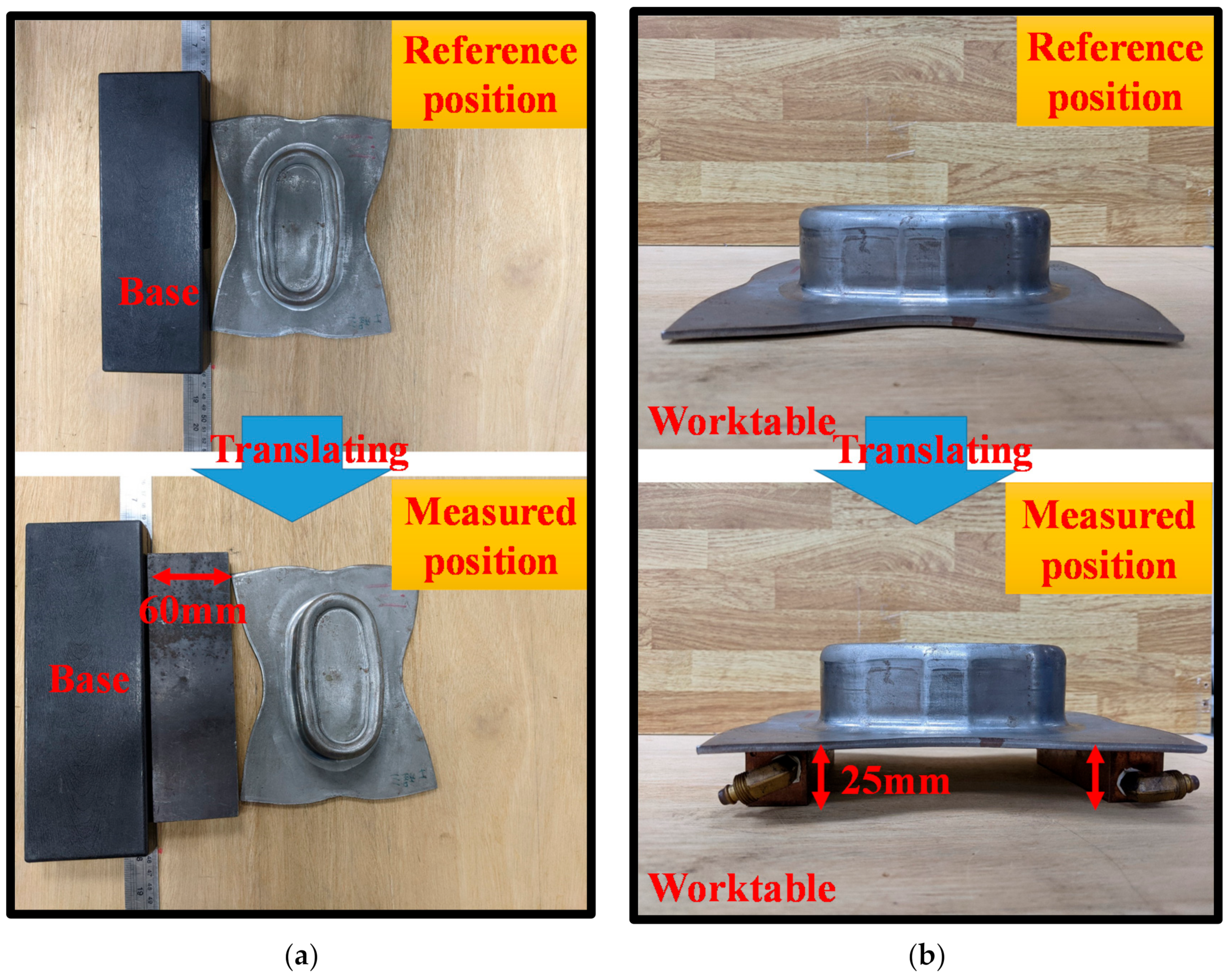
Firstly, the three translation axes X, Y, Z errors are considered. As shown in Figure 8a for the X and Y-axis, the workpiece is initially placed next to the base which is considered to be the reference position; afterward, place a block next to the base which will enable the workpiece to move a distance of 60mm (width of the block is 60mm). Then compared to the reference position, the workpiece is moved 60mm (the new position that needs to be measured); continue the experiment with other distances of 120mm, 180mm, and the other direction of −60mm, −120mm, −180mm. Figure 8b displays the experiment for Z-axis. Similar to the experiment of the X and Y-axis, this experiment also uses a block to move the workpiece but in the vertical direction (Z-axis) and the base now is the worktable. The experiment is carried out by using a block with height of 25mm. The distances of experiment are 25mm, 50mm, 75mm, 100mm, 125mm, and 150mm. Both in the reference and measured position, the workpiece point cloud is modeled for later recorded the error between the real distance and estimating distance.

Now, considering the rotation axes RX, RY, and RZ, the experiment setup for these axes is shown in Figure 9. The worktable is now recognized as the base and the reference position is where the workpiece is placed on the worktable. The experiment used the BOSCH rangefinder (Bosch, Germany) to estimate the angle. For the reference position, the rangefinder shows 0°. Thereafter, the workpiece is rotated by placing a block under its side. Now, the new position angle will be shown on the rangefinder. The experiment was conducted with the angles of 30°, 20°, 10°, −10°, −20°, and −30° for the RX and RY axes and 10°, 30°, 45°, 60°, 75°, and 90° for the RZ-axis.

The method of the pose estimation system of this study is shown in Figure 10a–f for the three translation axes of X, Y, and Z and the three rotation axes of RX, RY, and RZ. Similar to the description of the experiment setup above, the camera generates point clouds of the workpiece in both reference and measured positions to create the reference and measured cloud, respectively. In the figure, the blue point cloud is the reference point cloud, and the green point cloud is the cloud that needs to be measured for distance and angle. Each sub-experiment focuses on one axis in the total 6-DoF, and the estimated result is then compared with the real distance (or angle) to find the error.

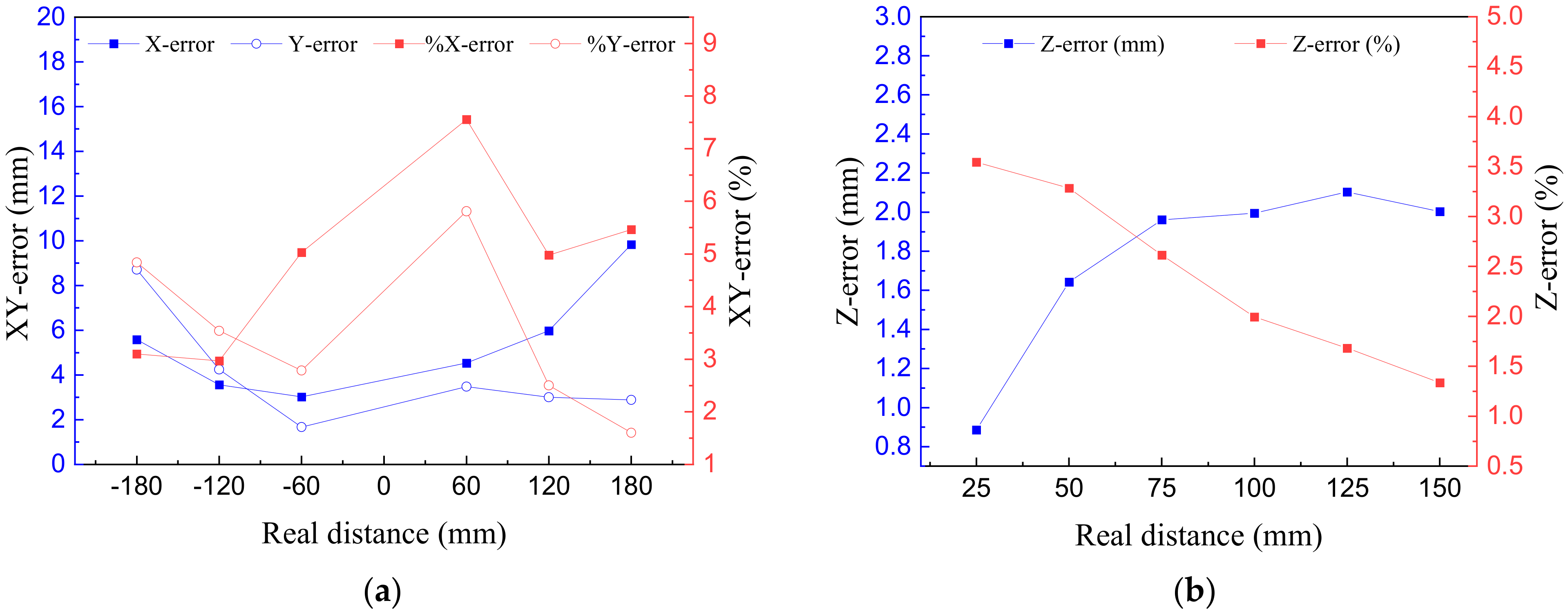
As shown in Figure 11, the translation error of the pose estimation of this study is considered to be reasonable and can be used in practical applications. Figure 11 confirms that the error of the translation axis ranges between 0.825 and 9.834 mm and 0.825~5.810%, and the average error is 5.417 mm and 4.850% for the X-axis, 4.001 mm and 3.513% for the Y-axis, and 1.570 mm and 2.214% for the Z-axis. The trend of Figure 11a points out that in the X and Y axes, the larger the distance between the reference and the measured points, the higher the error of the system. On the contrary, a smaller distance will lead to a higher error percent in the system. The same trend appears in the error of the Z-axis (Figure 11b).

Figure 12 demonstrates the rotation error of the system. For the RX and RY axes (Figure 12a), and the RZ-axis (Figure 12b), the errors are small if the real angle differences are small, but the error percent will increase when the angle differences decrease. The error and error percentage of the rotation axis range 0.13°~2.67° and 0.37~16.40%, respectively. The average error and error percentage of the RX-axis are 1.36° and 6.38%, respectively, the average error and error percentage of the RY-axis are 1.01° and 6.01%, respectively, and the average error and error percentage for the RZ-axis are 1.21° and 2.59%, respectively.

The second sub-experiment was conducted to examine the repetition accuracy of the pose estimation system. The setup of this sub-experiment is similar to the above experiments (as shown in Figure 8 and Figure 9). First, the workpiece is placed in the reference position, then it is moved to the new position that needs to be measured. However, in this experiment, the workpiece will be repositioned in all 6 axes. The measured position will be estimated 10 times; later, the data will be analyzed to find the repetition error of the pose estimation system.

As shown in Figure 13a, the translation error ranges 0.024~8.563 mm, which is 0.080~9.937%. The rotation error ranges 0.094°~2.908°, which is 0.314~9.923% (Figure 13b). The average error percentages of each axis are 3.905%, 3.182%, 5.087%, 6.013%, 6.189%, and 5.523% for the X, Y, Z, RX, RY, and RZ axes, respectively. The error values which were measured were all less than 10% and 9 mm. For the purpose of researching and developing, the pose estimation repetition error is adequate for the robot system to successfully pick up the object. All the measurements were performed independently; hence, each time, measuring repetition errors will result in a different set of errors and do not relate to any of the previous sets of measurements.

3.2. Robot Error Compensation Results

As mentioned in Section 2.4, we utilized the non-linear correction algorithm to compensate for the robot error. Figure 14 demonstrates the robot error experiment setup. First, the checkerboard (side of each square is 20 mm) is placed on the worktable; then, the worktable center point is considered to be the centroid and does not have an error (meaning in the worktable center point, $E_x=E_y=0$).

The worktable center point is set to be the base point, where the error is 0 for both the X and Y axes (Figure 15). The theory position of the other points (blue dots in 0) in the region of interest (red-dashed rectangle in 0) will be setup according to the base point and will be inputted into the controller. After the robot moves to the input position, the error is observed and measured, which is the displacement between the supposed input position (blue dot) and the actual moving position, by using the caliper. There are total of 198 points that were measured in the study.

Using the input positions, the matrix $A$ was calculated by recalling Equation (21). The matrix $B$ is the error measured between the input and the actual position, recalling Equation (22) to obtain matrix $C$—the coefficient matrix:

$$C=\left[\begin{array}{cc}1.03\times {10}^{-6}& -4.95\times {10}^{-7}\\ 2.25\times {10}^{-7}& 6.48\times {10}^{-7}\\ -4.55\times {10}^{-7}& -9.55\times {10}^{-8}\\ 3.69\times {10}^{-7}& 2.43\times {10}^{-7}\\ -2.21\times {10}^{-4}& 2.77\times {10}^{-4}\\ 3.11\times {10}^{-5}& -2.03\times {10}^{-4}\\ 2.98\times {10}^{-4}& 3.01\times {10}^{-4}\\ -0.20& -0.03\\ -0.12& -0.27\\ 44.69& 17.46\end{array}\right]$$

(28)

After applying the coefficient matrix to the calculation, the robot’s positioning accuracy significantly improved. 0a shows the robot error before using the compensation function. As can be seen, the error of the robot was very large, up to 39.69 mm on the X-axis and 45.45 mm on the Y-axis. The average error without correction was 10.55 and 20.86 mm on the X-axis and the Y-axis, respectively. On the other hand, 0b demonstrates the sharp enhancement of the robot positioning. Compared to before compensation, the average translation errors can now reduce by over 20 times with the X-axis and 40 times with the Y-axis, to 0.49 and 0.37 mm on average, respectively. The maximum errors were also downgraded to 3.47 and 2.50 mm for the X and Y axes, respectively.

Figure 16 visualizes the positions of all the points which were considered in the experiment. As shown in the figure, the real measurement positions (the red circle) of the input have a larger error compared to the input positions (the black square). However, after compensation using the non-linear correction algorithm, the robot positions (the blue triangle) have come closer to the input positions, and this statement is proven by the fact that the blue triangle points almost coincide with the black square points. This result indicates that the robot error can be solved by applying the coefficient function by software compensation.

3.3. Experiment of the Dynamic Stack Workpiece Feeding System

Figure 17 shows schematic diagram of dynamic workpiece feeding. When the signal starts to be transmitted and the pose estimation program is activated and completes the positioning of the object, the robot and the conveyor will move simultaneously so that while the conveyor is still moving, the robot will successfully pick up the object. The linear feed rate of the robot arm was set at 0.03 m/s. The distance between gripping position and scanning position was set at 0.5 m, and between gripping position and robot home position was set to 0.3 m. The dynamic task was accomplished by applying Equation (27) related to the velocity of the conveyor and the feed rate of the robot arm. Therefore, the velocity of the conveyor will be calculated as in Equation (29):

$$v_{conveyor}=\frac{FL\times \left|P_{scan}-P_{gripping}\right|}{\left|P_{robot}-P_{gripping}\right|}=\frac{0.3\times 0.5}{0.3}=0.5 \mathrm{m}/\mathrm{s}$$

(29)

After the camera finishes forming the point cloud, the program will predict the 6-DoF pose of the object based on that point cloud. If there is an object, the program will predict the location of the object, but if the object does not appear, the program will stop here. The position of the object will then be added with the conveyor’s travel distance, then transmitted over the Ethernet connection, and the robot arm will begin to pick up the object to the stamping machine. The rest of the task will be the stamping machine’s responsibility, and the pick-placing task is completed. The loop will continue if there are still objects to stamp.

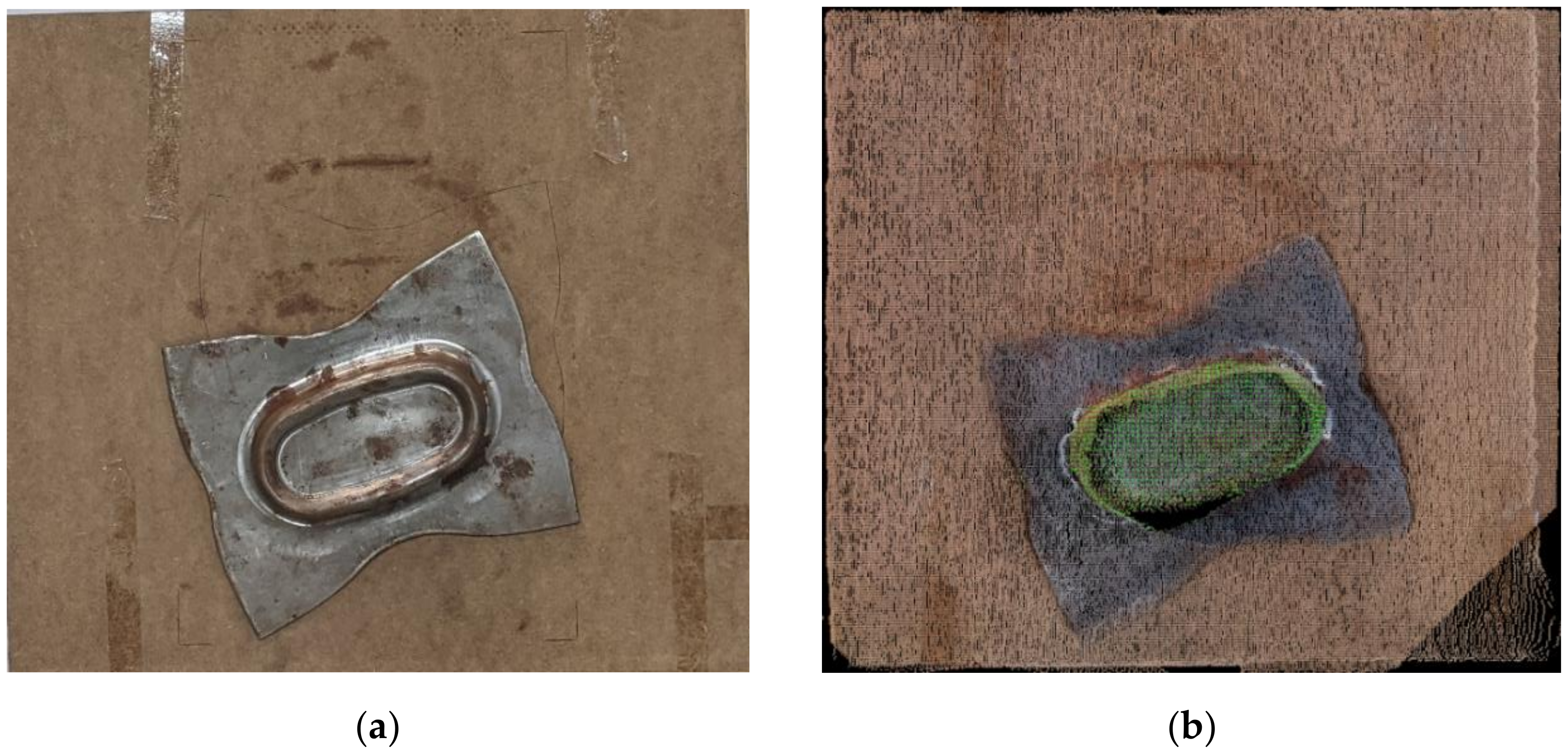
There were two experiments—the first with a single object and the second with a stack of two objects. Figure 18 and Figure 19 show cases where the robot successfully picked up the object to stamping die with single and piled objects, respectively. Figure 18a and Figure 19a show the workpieces that were placed in random positions, Figure 18b and Figure 19b show the scene point cloud of each case, Figure 18c and Figure 19c show the results of the pose estimation system, and finally, Figure 18d and Figure 19d show the images of the robot successfully picking up the object.

The results’ data are presented in

Table 1. Results of dynamic workpiece feeding compared with static workpiece feeding.

Item	Static		Dynamic
	Case 2	Case 1	Case 2	Case 1
Number of experiments	20	20	20	20
Successful case	18	19	13	14
Failure case	3	1	7	6
Successful rate (%)	90	95	65	70
Pose estimation time (seconds)	12	7	12	7

. Compared with static feeding (90% and 95%), dynamic feeding will have a significantly lower success rate—down to 65% in the case of 2 objects and 70% in the case of 1 object. The sudden drop in success rate is due to hardware limitations. The conveyor travel speed is not constant due to resistance and friction caused by the spindle shaft and the belt. The program’s object position estimation time will not change in this experiment.

4. Conclusions and Future Prospects

In this study, we have developed an automatic feeding system for dynamic workpieces of the stamping industry using a robotic arm and 3D cameras. The main contents covered in the study were divided into three sections. The first part was the formation of a 3D point cloud using depth cameras and combining two point clouds from these cameras with different angles setup into a complete point cloud by stereo calibration. The accuracy of the point cloud has been found to be satisfactory to perform computational tasks, with a 4.7 mm mean distance of point-to-point cloud error. In terms of the accuracy of object information in the point cloud, it has also been shown to be steady, with less than a 7% error in positioning and a 5% error in height. Using the generated point cloud as input for the pose estimation system was the second part of this study. We used several point cloud processing algorithms, with emphasis on Euclidean cluster extraction to segment the workpiece with other objects on the worktable, FPFH to evaluate the feature points of the target object as well as the reference object, and SAC-IA and ICP respectively, to align the target and reference point cloud and find the transformation matrix. The error of the estimated system was a high-grade error, with an average of less than 6 mm for the translation error and 3° for the rotation error. The repeatability error of the system was also kept stable, with an average of only 7% error. The last part was the transmission system with motion synchronization between the robotic arm and the conveyor to successfully pick up the objects. Before being used to pick up the object, the robotic arm will be calibrated by the nonlinear correction algorithm to find the appropriate adjustment coefficients that contribute to the accuracy of the manipulator. Compared to before compensation, the average translation errors were able to reduce by over 20 times with the X-axis and 40 times with the Y-axis, to 0.49 and 0.37 mm on average, respectively. The dynamic feeding experiment was performed with quite satisfactory success (>65%), despite the influence of limited hardware installation. This has proven to be viable in production with more invested equipment.

In the future, in addition to improving the device to meet the stability, another algorithm (potentially a Neural Network application algorithm) can be applied to calculate the position of the workpiece faster, to obtain real-time estimation. With the use of the fast refresh rate—Azure Kinect, the advantage of this study is that the scanning time for point cloud formation was within a second. However, using FPFH in combination with SAC-IA and ICP to compare and provide estimated locations of a workpiece requires a minimum of seconds. Therefore, the study can hardly be achieved in real-time. Besides, to increase the success rate of dynamic workpiece grabbing, as mentioned above, it is also necessary to have more stable devices. Since the depth sensors have a certain operating temperature (10–25 °C), the accuracy of processing point cloud data can be affected if the temperature is high. As a result, the workpiece modeling has to be carried out before undergoing the austenitization process. An experiment examining the influence of thermal radiation on modeling will be performed in future work. In the end, the study is only a simulation of a feeding system, and some other devices, which have the effect of supporting production automation, such as sensors measuring product quality and cameras playing the role of an observation and alarm alert when the system has problems, can be integrated to create a full-cycle stamping process. The robotic arm is also not the only option of stamping workpiece feeding automation, and other kinematic architectures should be applied in terms of size, payload, and preferences.

References

- Srasrisom, K.; Srinoi, P.; Chaijit, S.; Wiwatwongwana, F. Modeling, analysis and effective improvement of aluminum bowl embossing process through robot simulation tools. Procedia Manuf. 2019, 30, 443–450. [Google Scholar] [CrossRef]
- Karbasian, H.; Tekkaya, A.E. A review on hot stamping. J. Mater. Process. Tech. 2010, 210, 2103–2118. [Google Scholar] [CrossRef]
- Handreg, T.; Froitzheim, P.; Fuchs, N.; Flügge, W.; Stoltmann, M.; Woernle, C. Concept of an automated framework for sheet metal cold forming. In Proceedings of the 4th Kongresses Montage Handhabung Industrieroboter, Berlin/Heidelberg, Germany, 3 May 2019; pp. 117–127. [Google Scholar]
- Tölgyessy, M.; Dekan, M.; Chovanec, Ľ.; Hubinský, P. Evaluation of the Azure Kinect and Its Comparison to Kinect V1 and Kinect V2. Sensors 2021, 21, 413. [Google Scholar] [CrossRef]
- Anwer, A.; Ali, S.S.A.; Khan, A.; Meriaudeau, F. Underwater 3-D Scene Reconstruction Using Kinect v2 Based on Physical Models for Refraction and Time of Flight Correction. IEEE Access 2017, 5, 15960–15970. [Google Scholar] [CrossRef]
- Hänsch, R.; Weber, T.; Hellwich, O. Comparison of 3D Interest Point Detectors and Descriptors for Point Cloud Fusion. In Proceedings of the Photogrammetric Computer Vision, Zürich, Switzerland, 5–7 September 2014. [Google Scholar]
- Guo, N.; Zhang, B.H.; Zhou, J.; Zhan, K.T.; Lai, S. Pose estimation and adaptable grasp configuration with point cloud registration and geometry understanding for fruit grasp planning. Comput. Electron. Agric. 2020, 179, 105818. [Google Scholar] [CrossRef]
- Zhang, Y.; Meng, J.; Sun, Y.; Wang, Q.; Wang, L.; Zheng, G. Research on the cooperative work of multi manipulator in hot stamping production line. In Proceedings of the 5th International Conference on Advanced Design and Manufacturing Engineering, Shenzhen, China, 19–20 September 2015. [Google Scholar]
- Lindner, M.; Schiller, I.; Kolb, A.; Koch, R. Time-of-Flight sensor calibration for accurate range sensing. Comput. Vis. Image Underst. 2010, 114, 1318–1328. [Google Scholar] [CrossRef]
- Rathnayaka, P.; Baek, S.-H.; Park, S.-Y. An Efficient Calibration Method for a Stereo Camera System with Heterogeneous Lenses Using an Embedded Checkerboard Pattern. J. Sens. 2017, 2017, 1–12. [Google Scholar] [CrossRef] [Green Version]
- Fischler, M.A.; Bolles, R.C. Random sample consensus: A paradigm for model fitting with applications to image analysis and automated cartography. Commun. ACM 1981, 24, 381–395. [Google Scholar] [CrossRef]
- Rusu, R.B. Semantic 3D Object Maps for Everyday Manipulation in Human Living Environments. KI Künstliche Intell. 2010, 24, 345–348. [Google Scholar] [CrossRef] [Green Version]
- Saval-Calvo, M.; Azorin-Lopez, J.; Fuster-Guillo, A.; Garcia-Rodriguez, J. Three-dimensional planar model estimation using multi-constraint knowledge based on k-means and RANSAC. Appl. Soft Comput. 2015, 34, 572–586. [Google Scholar] [CrossRef] [Green Version]
- Hajebi, K.; Abbasi-Yadkori, Y.; Shahbazi, H.; Zhang, H. Fast Approximate Nearest-Neighbor Search with k-Nearest Neighbor Graph. In Proceedings of the 22nd International Joint Conference on Artificial Intelligence, Barcelona, Spain, 16–22 July 2011; pp. 1312–1317. [Google Scholar]
- Rusu, R.B.; Blodow, N.; Beetz, M. Fast Point Feature Histograms (FPFH) for 3D registration. In Proceedings of the 2009 IEEE International Conference on Robotics and Automation, Kobe, Japan, 12–17 May 2009; pp. 3212–3217. [Google Scholar]
- Rusu, R.B.; Marton, Z.C.; Blodow, N.; Beetz, M. Learning informative point classes for the acquisition of object model maps. In Proceedings of the 2008 10th International Conference on Control, Automation, Robotics and Vision, Hanoi, Vietnam, 17–20 December 2008; pp. 643–650. [Google Scholar]
- Shi, X.; Peng, J.; Li, J.; Yan, P.; Gong, H. The Iterative Closest Point Registration Algorithm Based on the Normal Distribution Transformation. Procedia Comput. Sci. 2019, 147, 181–190. [Google Scholar] [CrossRef]
- Besl, P.J.; McKay, N.D. A method for registration of 3-D shapes. IEEE Trans. Pattern Anal. Mach. Intell. 1992, 14, 239–256. [Google Scholar] [CrossRef]
- Ji-ming, Z. Research on nonlinear correction algorithm of two-dimensional PSD based on ploynominals. Ship Sci. Technol. 2019, 41, 89–93. [Google Scholar]
Figure 1.
Experiment device setup of stereo vision scanning for dynamic workpiece.
Figure 2.
Calibration model of a camera in the dynamic workpiece modeling application.
Figure 3.
Schematic diagram of two cameras’ stereo calibration for dynamic workpiece modeling.
Figure 4.
Effect of object segmentation in the study of dynamic workpiece feeding.
Figure 5.
Effect area diagram of estimated feature point for the dynamic workpiece using FPFH.
Figure 6.
Construction of the target object gripping pose.
Figure 7.
Initial positions of dynamic scanning region and robot gripping system on the conveyor.
Figure 8.
Setup of standard positions for different estimation poses of the dynamic workpiece using a predetermined dimension block for (a) the X-axis and Y-axis and (b) the Z-axis.
Figure 9.
Setup of standard rotation angles for different estimation poses of the dynamic workpiece using the professional laser rangefinder of BOSCH.
Figure 10.
Building reference point cloud models of each 6-DoF pose for estimating measured clouds of the dynamic workpiece in the (a) i-axis, (b) Y-axis, (c) Z-axis, (d) RX-axis, (e) RY-axis, and (f) RZ-axis.
Figure 11.
Translation errors of workpiece modeling at different estimated poses for the (a) XY-axis and the (b) Z-axis.
Figure 12.
Rotation errors of workpiece modeling at different estimated poses for (a) the RX and RY axes and (b) the RZ-axis.
Figure 13.
Repetition error and error percentage of the 6-DoF pose estimation system: (a) translations of X, Y, and Z axes, and (b) rotations of RX, RY, and RZ axes.
Figure 14.
Initial position of robot and conveyor and gripping position.
Figure 15.
Positioning errors of the robot on the XY plane (a) before compensation and (b) after compensation.
Figure 16.
Position differences of the robot before and after compensation using the non-linear correction algorithm for robot pick-place.
Figure 17.
Flow chart of pose estimation and robot control programs for the dynamic workpiece feeding control system.
Figure 18.
Dynamic single object on the conveyor (a) in a random position, (b) automatically identifying the RGB point cloud scene of the object, (c) estimating the object 6-DoF poses, and (d) the robot grasping the object in the dynamic experiment.
Figure 19.
Dynamic piled workpieces on the conveyor (a) in a random position, (b) automatically identifying the RGB point cloud scene of a top object, (c) estimating the object 6-DoF poses of a top object only, and (d) robot grasping the top object in the dynamic experiment.