Strategic Supply Chain Planning for Food Hubs in Central Colombia: An Approach for Sustainable Food Supply and Distribution

Featured Application

This work considers a real-life problem posed by public institutions of Colombia responsible for the design and implementation of food supply master plans. As such, the results presented in this paper will likely have a direct impact in public policies that consider both ends of a fresh food supply chain: Farmers in the countryside and end consumers at the major demand centers.

Abstract

This paper investigates the problem of sustainable rural supply and urban distribution of fresh food products in central Colombia. Paradoxically, while farmers in the countryside suffer from poverty due to the low profitability of the agricultural activity, inhabitants at urban centers pay high prices for fresh and nutritious foods. In this work, we propose a supply chain system and a business model based on food hubs located on existing (and often abandoned) public facilities in the central region of Colombia. There are many examples in which the hub strategy has facilitated trade and logistics in supply chains. However, few studies consider the particularities of the presented case. We study a business strategy through a mathematical model which considers both the sustainable and efficient operation of the food hubs and better trading conditions for farmers. We propose a variant of the competitive hub location problem adapted to this case study. We tested the model under different scenarios such as changes in the attractiveness parameters, operation costs, and profit margins. The results suggest that if hubs are able to attract farmers, the model can be both sustainable for the hub concessionaires and for the farmers.

1. Introduction

Modern supply chains must not only be cost efficient and guarantee quick responses to their customers, but must also guarantee the alignment of the interests of its stakeholders and the equitable distribution in costs and margins. The location of facilities is a strategic decision that has a significant influence in supply chain performance that can create a competitive advantage in commercial supply chains and improve coverage in public supply chains. A good facility location strategy can also significantly decrease the transportation and emission costs, and mitigate its environmental impact.

This research addresses a real problem of a fresh food supply chain in rural areas of Central Colombia. This problem is currently under study by RAP-E-(Administrative Office for Special Regional Planning—in Spanish), a region-wide public institution responsible for designing and implementing public policies for its food supply master plan. As such, this paper not only fed its models with real data, but also received valuable inputs from the senior RAP-E-management.

The fresh food supply chain studied in this paper is typical in emerging economies. In general, a large number of fragmented and disperse farmers supply fresh products to urban areas. These farmers rely heavily on intermediation that increases the prices paid by the final customers and create handling problems and food losses [1]. In central Colombia, this issue of intermediation has been long discussed, and several actions have been devised by local and central governments to reduce or eliminate its impact [2]. The most prominent was the construction of urban food hubs in Bogotá, the country capital [2]. This strategy was designed to directly connect farmers and shop owners with the support of an information system. The main idea was that shop owners placed orders directly to farmers through an Internet platform and a third-party logistics (3-PL) company were responsible for the hub operation and for the transportation of the agricultural products from the countryside to the city hubs. Important efforts were made by the mayor office of Bogotá to create networks of both shop owners and farmers and to educate them in the best commercialization and technology practices. Unfortunately, this strategy failed due to several reasons that included lack of Internet connectivity and poor logistics and business considerations [1]. No major 3-PL company participated in the concession bid, and the farmers’ and shop owners’ networks disbanded after a few attempts. A recent research [1] showed that the best strategy in terms of profits was intermediation.

More recently, the COVID 19 pandemic has seen a number of apps supported by Industry 4.0 technologies (e.g., [3,4]) which link farmers directly with both store owners and final consumers. As of today, these efforts have been modest at best and the vast majority of products is still traded through middlemen. There are several reasons, as pointed out in [5]: Middlemen play a significant role in this type of supply chain by matching supply and demand and shortening transaction times [6]. They also have a close relationship with farmers, as they, farmers, and middlemen, often live in the same region and share traditions and culture [5,7]. This fragmented farming system is also very inefficient in logistics and environmental terms: For example, an estimate of 12,000 trucks arrive daily to Bogotá with fresh food products. Most of these trucks are small and old 10-ton vehicles that travel half-loaded from locations within a 200 Km radius [1,8].

A common strategy to mitigate intermediation and to help small and mid- size farmers access larger markets is the development of regional food hubs. This strategy has been implemented in both first world [9,10] and in emerging countries [11,12]. The U.S. Department of Agriculture (USDA) defines a food hub as “a centrally located facility with a business management structure facilitating the aggregation, storage, processing, distribution, and/or marketing of locally/regionally produced food products” [13]. Hubs act both as supply consolidators and distributors. As such, hubs can also facilitate access to healthy foods to vulnerable populations by redirecting food flows to underserved areas that could hardly be reached out to with direct links [11]. In Colombia, the CONPES 3982—National Policy of Logistics of January 2020 document, establishes as one of its strategic pillars, the adoption of specialized logistics infrastructures—(ILEs in Spanish), which can play a prominent role as articulators between cargo and transport modes and providing value-added logistics services.

Food hub location problems have attracted researchers from different disciplines such as operations research [9], economics [14,15], and social sciences [16]. This paper focuses on the hub location problem adapted to the food systems in the central region of Colombia. Accordingly, we propose the following research questions:

• RQ1: “How rural food hubs in emerging economies can become a sustainable strategy to improve farmer’s access to urban markets?”
• RQ2: “Where should a network of food hubs be located with the goal of both maximizing farmer coverage and minimize logistics costs?”
• RQ3: “How the transportation and emissions costs are impacted by the hub strategy?”

This paper addresses the above three questions. The main contributions of this work can be summarized as follows:

• A new mathematical model of competitive hub locations that incorporates constraints specific of the situation of farmers in emerging countries with provisions for a sustainable operation.
• A combination of heuristics with the mathematical model aimed at solving realistic size problems.
• An extensive analysis of scenarios with recommendations that can be used for public policies.

2. Context

The central region of Colombia encompasses 5 administrative departments: Boyacá, Cundinamarca, Meta, Tolima, and Huila, and the Bogotá Capital District as a special administrative unit.

Table 1. The central region in figures.

Department	Population	% Colombia	% Region
Bogotá D.C	7,181,469	14.9	50.3
Boyacá	1,135,698	2.4	8.0
Cundinamarca	2,792,877	5.8	19.6
Meta	919,129	1.9	6.4
Tolima	1,228,763	2.5	8.6
Huila	1,009,548	2.1	7.1
Totals	14,267,484	29.6%	100%

shows the composition according to population (according to figures from the most recent population census in 2018, Colombia has over 48 M habitants [17]):

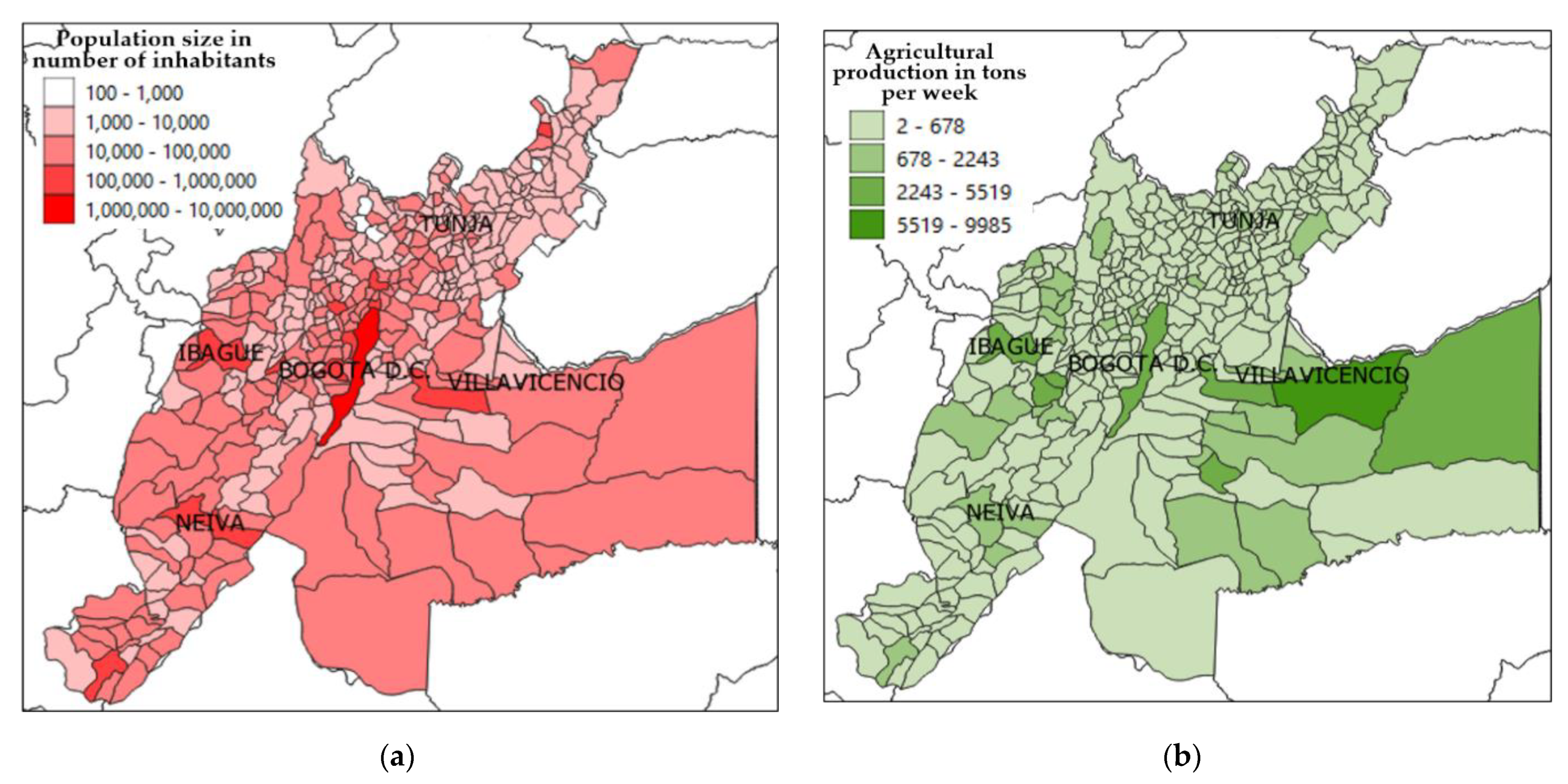
Figure 1 illustrates the population distribution according to the areas of the region and provides recent figures of the agricultural production. Bogotá is the most densely populated municipality, with more than 200,000 habitants per square kilometer, followed by Cundinamarca with between 100.1 to 200 inhabitants per square kilometer, and, Boyacá, Meta, Tolima, and Huila with between 50.1 to 100 inhabitants per square kilometer.

The population of the Central Region of Colombia is estimated in approximately 2.1 million inhabitants (14% of the country), of which 75% are rural. The region concentrates 26% of the agricultural production of the country (agriculture, livestock, hunting, forestry, and fishing).

The central region has a wide variety of climates. The Andes cordillera that runs south-north splits the central region in three sub-regions: The hot and humid valleys in the west, the mountainous area in the central part, and the semi-arid plains in the east. The mountainous region itself presents a wide variety of ecosystems: Dense cloud forests, high plains, and semi-deserts to name a few.

These climates create an excellent environment for agricultural activities. The central region of Colombia, in terms of the agricultural economic activity, contributes with approximately 30% to the GDP of Colombia. This contribution has remained relatively constant in the last 15 years. The central region produces 26% of Colombia’s food. The main agricultural food products are potato, plantain, rice, sugar cane, and corn.

Table 2. Hectares cultivated and production of the main products of the Central Region.

Department	Production (Ha)	% Colombia
Rice	185,688	15.9%
Corn	167,086	22.0%
Potato	121,632	4.4%
Sugar cane	66,074	16.1%
Plantain	52,025	9.0%

shows the total hectares planted and the agricultural production in tons in the central region. This information was compiled from [18].

According to data from the latest available National Logistics Survey (2018) [19], the operating and logistics costs of the agricultural industry in Colombia account for 12.8% of the final price (below the national average which is 13.5%), where the main components of such operation costs are storage (35.9%), transportation (33.3%), overhead (27.7%), and customer service and other costs (3.1%).

A factor that contributes to the reduction of storage costs is to improve inventory turnover (in days), according to the same survey [19]. The agricultural industry reports 11.8 days of inventory in raw materials and agricultural supplies and 24.4 days in finished product, while supply days are 20.5, and in distribution, 16.7. Likewise, in terms of transportation costs, reducing the traveled distance can clearly contribute to the reduction of operating costs. In the Colombian agricultural industry, trucks and other cargo vehicles average 2744 km/month on intercity journeys and 2066 km/month on urban journeys. In relation to the quality of deliveries (deliveries on time, error-free documentation, and so forth), for the agricultural industry the performance rate is around 79.8%, which can be considered very low [19]. The main reported problems were damage to the goods (food loss), transport delays and customer-related delivery problems [19].

The above figures show that a food hub strategy specialized in the supply, storage, and distribution of agricultural products in the central region of Colombia, can be an opportunity to reduce (i) the number of intervening actors, (ii) the days of inventory, and (iii) the traveled distance.

3. Literature Review

In this section, we explore the mathematical foundations of hub location problems. This is a particular case of the facility location problem (FLP) that consists of both establishing the location of one or more facilities and the assignment of customers to such facilities [20]. Most problems studied in the literature derive from the classical p-medians, fixed charge and set covering problems [20]. The p-medians consist of establishing the location of exactly p facilities among a set of n > p possible sites with the objective of minimizing the total weighted distance. The fixed charge cost is a natural extension of the p-medians in which the number of facilities is a decision variable itself. In this model, in addition to transportation costs, there are fixed charge costs associated with the opening/operation of the facilities. The set covering problem (SCP) differs from the above two in the sense that the objective is minimizing the number of facilities subject to the constraint that all customers must be served [21]. Facilities can only serve customers located within a predefined radius of influence (i.e., customers are covered). A different approach to coverage are the Huff’s gravity [22] and the logistics regression (logit) [23] models. These models, instead of having the sharp coverage distinction of the SCP (i.e., covered or not), establish the probability that a customer patronizes a facility. This probability is related to some measure of attractiveness of the facility. The first papers considered only retail stores [22]. Later models included other services [24].

There are many variants of the FLP and it is not the purpose of this paper to cover them all. For a complete review, please see [25,26]. An extension of the FLP used in this paper is the competitive facility location problem in which the decision maker does not have control on the choices of the customers, but rather has estimations of their shopping behavior [27,28,29]. In general, these choices are modeled through either the Huff or the logit formulas. Most papers consider Mixed Integer Linear Programming (MILP) formulations and use either standard MILP solvers [30] or decomposition algorithms [31,32]. Other approaches use metaheuristics algorithms [33,34,35].

Facility location models are also common for fresh food and agriculture supply chain design [36,37]: This topic of has attracted many researchers that have addressed multiple problems [38,39]. Some examples related to emerging countries are: Villegas et al. [12] proposed a bi-level algorithm for the location of purchasing centers in the coffee belt region of Colombia. The two objectives considered were the cost minimization and the coverage maximization. Amorim et al. [40] presented a MILP model for supply chain design with JIT planning and scheduling with perishability constraints. Orjuela-Castro [8] proposed a MILP model for the location of fruit processing centers in the central region of Colombia. This model included humidity and temperature related constraints of the potential sites. Suraraksa and Shin [41] introduced a MILP model for the network design of urban distribution centers of fruits and vegetables in Bankok (Thailand). They investigated not only location, but also vehicle routing extensions. Later, Granillo [42] presented a real-life application model for the location of a catering distribution problem in urban schools in Mexico considering waiting times. In most of these papers, the objective function was the cost minimization including fixed, transportation, and other costs related to quality, and/or delivery. Several extensions in food supply chain combine facility location with combinatorial another problem: Examples are the location and routing [43,44] and the inventory location [45] problems.

A special case is the hub location problem: In this problem, entities travel between predefined origin and destination (OD) nodes. These entities can either travel directly between OD nodes or through a hub. These hubs may facilitate the flow of entities, and reduce transportation costs due to economies of scale [9]. Clearly, the hub location is not restricted to supply chains. Many applications exist in the telecommunication, airline, and urban transportation sectors [46,47]. The hub location involves several decisions: (1) Selecting a subset of hubs among a set of candidate locations, (2) determining inflows and outflows at the selected hubs, and (3) determine the transportation modes. A variant, closely related to this research, is the competitive hub location problem [24,46,48]. In the competitive hub location problem, a company intends to establish new hubs where there are already other competitors including the company’s own hubs. The objective is generally to maximize profit, which involves two terms: (1) The company’s revenue, which is proportional to the attracted demand, and (2) fixed and variable costs [46].

The mathematical problem of perishable food hubs has been little studied: Among the few works, Etemadnia et al. [9] proposed a MILP formulation for regional food hubs in the United States, which is solved in two phases with a linear relaxation in the first phase to filter our non-promising nodes and a second phase that included integer and binary variables. Later, Musavi et al. [49] presented a multi-objective perishable food hub location and scheduling problem for sustainable supply chains. Finally, Gharehyakheh et al. [50] presented a multi-objective formulation for the case of distribution of perishable foods considering emissions and shelf life. The last two references use Multi Objective Evolutionary Algorithms (MOEAs).

Most works on food hub and food supply chains consider decisions based on centralized control of all links: Suppliers, hubs, and retailers [44,49,50,51]. This is not realistic in the studied case: First, farmers in central Colombia have choices to sell and distribute their products. Second, in the literature of supply chains, the demand must be fully or partially satisfied [49,52]. In this paper, we assume that the hub management makes decisions as to where to deliver the products based on some parameter of attractiveness of the trading point (i.e., the city wholesaler) as in [26,27,46] Normally, this decision has to do with several factors such as familiarity with the trading point, or with the probability of finding customers. We make the reasonable assumption that the demand of each city is far larger than the quantities that the hubs can deliver. After all, these regional hubs in the central region of Colombia are facilities located in small-to-medium size towns with limited capacity (the largest with around 600 tons) and for instance, the total demand of the country capital Bogotá alone is over 40,000 tons per day.

In the problem studied in this paper, we have a combination of centralized and decentralized decisions. The purchasing center has control on the operation of the facilities and of the distribution to the cities (i.e., outbound logistics); however, since farmers are not contractually bound by the food hubs, one goal is to attract farmers and therefore the agricultural production in the most profitable and sustainable way. As such, farmers are customers of the food supply chain system and therefore a portion of their yield is expected to be captured by the food hubs.

Our work has both obvious similarities and important differences with the competitive hub location problem: On the similarities side, farmers may choose to travel to the food hubs or sell their products directly to middlemen, wholesalers, or to final customers as in [1,6]. The decision will be made based again on some measure of attractiveness [7]. The objective function (maximizing profit) presented in this paper is consistent with those of the hub facility location literature (e.g., [27,46,53]). In terms of differences, the proposed food hub model is more than a consolidation and storage facility where the product arrives and then it is re-distributed. In our proposal, the hub company would also purchase the product directly to the farmers (as suggested in [2]). Many successful cases in emerging countries use this business model (e.g., [11,12] to name a few) because of culture and traditions of the social network. Second, there is not a predefined destination for the fresh food products as this is a management decision as explained above. Finally, in our model, farmers do not bear the cost of traveling from the hub to the cities. This cost is borne by the hub concessionaire.

4. Materials and Methods

The problem studied in this paper can be summarized as follows: Given a set of famers, a set of candidate hub locations, and a set of customers (represented as cities or towns), locate the best subset of hubs in order to maximize profits. On one hand, the hubs’ location must be attractive to farmers (i.e., close to them) and on the other hand, these hubs should also be located close to the demand points to reduce transportation costs. Attracting farmers also has the benefit of economies of scale on transportation and on fixed operation costs.

4.1. Data Preparation

In this section we provide the details of the proposed mathematical model. We study the five largest agricultural chains defined by RAP-E-. In this context, an agricultural chain is defined as a set of agricultural food products which share some special characteristics such as temperature requirements during handling/transportation and packing. As a result, products of the same agricultural chain can be transported in the same vehicle. Appendix A shows the description of the agricultural chains.

Table 3. Data collection for modeling the problem.

Entity	Data	Source
Farmers	Annual yield of 54 agricultural products grouped in 5 agricultural chains Approximate geographical location 1 Distances to logistics hubs	RAP-E-
Demand points	Annual intake of fresh foods per person-day Geographical location Population	RAP-E-, DANE [17]
Logistics operators	Capacity in tons Monthly cost of operation/opening Geographical location Distances to farmers/demand points Cost of transportation (fixed & variable) Emissions	RAP-E- Ministry of Transportation [54] Ministry of Environment [55] Corabastos (bulletin of prices) [56]

¹ Georeferenced location and area of the production zones.

shows the data used in the models and their sources. A description follows next:

Figure 2 shows the location of the 30 selected potential hub locations in the central region.

4.2. Model Formulation

We developed a model based on the Hub Location Competitive model formulated in [46]. Our model considers that farmers can choose a buyer not only among available hubs’ potential locations, but among the demand points to sell their products. In this paper, the probability of a farmer choosing the products’ destination is given by the Huffs gravity model that involves population size and distance as the main factors. The original Huff’s formula establishes the probability that a customer selects a market. In this context, we made the reasonable assumptions that the main criteria for market selection are size (i.e., the probability of finding buyers is greater) and distance (i.e., the greater the distance, the more costly and the less familiarity with the market).

As such, and according to the Huff’s formula, the probability $y_{ij’}$ that a seller $i$ select a market $j’$ is given by Equation (1):

$$y_{ij’}=\frac{\frac{w_{j’}^{\delta }}{d_{ij’}^{\gamma }}}{{{\displaystyle \sum }}_{j\in J}\frac{w_j^{\delta }}{d_{ij}^{\gamma }}} \forall h\in H;j\in J$$

(1)

where $d_{ij’}$ is the distance between seller $i$ and market $j’$, $w_{j’}$ is the size of market $j’$ and $\gamma$ and $\delta$ are exponents greater or equal to 0 to be determined.

In addition, we used this choice model to determine the quantities to be delivered by a hub to its potential customers. The same rationale can be applied to the hub management when choosing markets to sell their products. It means we use a double selection, one in each echelon of the supply chain. We regarded a set of production points (farmers’ locations) $i\in I$ that have to choose between sending directly to a demand point $j\in J$ or use an available intermediary (set of hubs) $h\in H$. The selection is made with a probability $y_{ih}$ that depends on the distance between the farmer and the hub $d{’}_{ih}$ or the demand point ${\widehat{d}}_{ij}$ and the population size of hub municipality ${\widehat{w}}_h$ or demand point city $w{’}_j$. Both factors, distance and population, define corresponding sensitivity exponents $\gamma$ and $\delta$, respectively. With the probability variable $y_{ih}$, we defined the quantities of each product $k\in K$ to send to each available open hub. The other important aspect that we considered in this model is the selection of transportation vehicles. In the central Colombian case, agricultural products are transported in mainly three types of trucks: Trailer trucks (32 ton), 2-axle (16 ton) trucks, and “turbo” trucks (smaller 4.5 ton) trucks. According to the information of the Ministry of Transportation [57], most trucks travel around 50% loaded. For this reason, we set a minimum occupancy of 50% for the larger trucks in our model.

Table 4. Definition of indices and parameters.

Sets
$I$	Farmers’ locations.
$H$	Potential location of hubs.
$J$	Demand points’ locations.
$K$	Products.
$L$	Agricultural chains’ classification.
$V$	Type of vehicle.
Parameters
$c_h$	Operation fixed cost of hub $h$.
$q_h$	Capacity of hub $h$.
$margi{n}_k$	Unit profit margin of product $k$.
$\widehat{c_v}$	Operation fixed cost for each vehicle type $v$.
$c_v$	Variable cost per kilometer and ton of each vehicle type v.
$e_v$	Average carbon dioxide emission in tons per kilometer for vehicle v.
$c_v^{’}$	Unit cost of carbon dioxide emission per kilometer by vehicle v.
$q_v^{’}$	Capacity of vehicle v.
$mi{n}_v$	Minimum occupancy of vehicle v (%).
${\widehat{w}}_h$	Population of hubs’ location h.
$w{’}_j$	Population of demand point j.
$d{’}_{ih}$	Distance between farmer i and hub h.
${\widehat{d}}_{ij}$	Distance between farmer i and demand point j.
$d_{hj}$	Distance between hub h and demand point j.
$o_{ki}$	Weekly quantities of product k by sold by farmer i.
$a_{kl}$	Binary parameter that establishes if product k belongs to agricultural chain l.
$\gamma$	Sensitivity exponent for the distance between farmers and hubs.
$\widehat{\gamma }$	Sensitivity exponent for the distance between hubs and cities.
$\delta$	Sensitivity exponent for population factor.
$p_{hj}$	Probability of hub h of selecting demand point j.

and

Table 5. Definition of decision variables.

Decision Variables
$x_h$	Binary variable if hub location h is open
${\widehat{s}}_{ki}$	Weekly quantities (tons) of product k sent from farmer i to demand points
$y_{ih}$	Probability of farmer i of choosing to go to hub h
$s_{kih}$	Weekly quantities (tons) of product k sent from farmer i to hub h
$s{’}_{khjv}$	Weekly quantities (tons) of product k sent from hub h to demand point j in vehicle v
$truc{k}_{vhjl}$	Number of vehicles v with products of agricultural chain l sent from hub h to demand point j

show the definition of sets, parameters, and variables.

The objective function is to maximize the hubs’ net profit considering a gross profit $margi{n}_k$ for each product, fixed costs of operating a hub $c_h$, fixed $\widehat{c_v}$ and variable $c_v$ costs of transportation, and emission costs of carbon dioxide $c_v^{’}$. The costs of transportation and emissions are associated with each type of vehicle $v\in V$. Equation (2) corresponds to the objective function formulation.

$$\begin{array}{c}Max {\displaystyle \sum }_{k\in K}{\displaystyle \sum }_{h\in H}{\displaystyle \sum }_{j\in J}{\displaystyle \sum }_{v\in V}margi{n}_k{s^{\prime }}_{khjv}-({\displaystyle \sum }_{h\in H}{c}_h{x}_h+{\displaystyle \sum }_{l\in L}{\displaystyle \sum }_{h\in H}{\displaystyle \sum }_{j\in J}{\displaystyle \sum }_{v\in V}\widehat{c_v}truc{k}_{vhjl}+{\displaystyle \sum }_{k\in K}{\displaystyle \sum }_{h\in H}{\displaystyle \sum }_{j\in J}{\displaystyle \sum }_{v\in V}{c}_v{d}_{hj}s{\text{'}}_{khjv}\\ +{\displaystyle \sum }_{l\in L}{\displaystyle \sum }_{h\in H}{\displaystyle \sum }_{j\in J}{\displaystyle \sum }_{v\in V}{c}_v^{\text{'}}{e}_v{d}_{hj}truc{k}_{vhjl})\end{array}$$

(2)

The constraints are defined as follows. Constraint set Equation (3) determines a farmer’s probability to select a hub or a demand point according to the Huff’s gravity model. Constraint set Equation (4) establishes the quantities of product $k$ delivered by farmer $i$ to hub $h$. Constraint set Equation (5) corresponds to the balance of quantities of product $k$ traded by farmer $i$. Constraints set Equation (6) is the hub capacity constraint. Constraint set Equation (7) guarantees that the quantities delivered from hubs to the demand point are not greater than the quantities received by the hub. Constraint sets Equations (8) and (9) ensure the minimum and maximum occupancy levels per vehicle type. Constraint set Equation (10) determines the quantities sent from hub $h$ to each demand point $j$ according to the gravity model’s probability. Constraint sets Equations (11) and (12) refer to the non-negativity and binary constraints of the decision variables.

$$y_{ih}=\frac{\frac{{\widehat{w}}_h^{\delta }}{{d^{\prime }}_{ih}^{\gamma }}{x}_h}{{{\displaystyle \sum }}_{h’\in H}\frac{{\widehat{w}}_{h’}^{\delta }}{{d^{\prime }}_{ih’}^{\gamma }}{x}_{h’}+{{\displaystyle \sum }}_{j\in J}\frac{{w^{\prime }}_j^{\delta }}{{\widehat{d}}_{ij}^{\gamma }}} \forall i\in I;h\in H$$

(3)

$$o_{ki}{y}_{ih}=s_{kih} \forall k\in K;i\in I;h\in H$$

(4)

$${\displaystyle \sum }_{h\in H}{s}_{kih}+{\widehat{s}}_{ki}=o_{ki} \forall i\in I;k\in K$$

(5)

$${\displaystyle \sum }_{k\in K}{\displaystyle \sum }_{i\in I}{s}_{kih}\le q_h{x}_h \forall h\in H$$

(6)

$${\displaystyle \sum }_{i\in I}{s}_{kih}\ge {\displaystyle \sum }_{j\in J}{\displaystyle \sum }_{v\in V}{s^{\prime }}_{khjv} \forall k\in K;h\in H$$

(7)

$${\displaystyle \sum }_{k\in K}{a}_{kl}{s}_{khjv}^{’}\le q_v^{’}truc{k}_{vhjl} \forall v\in V;h\in H;l\in L;j\in J$$

(8)

$${\displaystyle \sum }_{k\in K}{a}_{kl}{s}_{khjv}^{’}\ge q_v^{’}\left(truc{k}_{vhjl}-\left(1+mi{n}_v\right)\right) \forall v\in V;h\in H;l\in L;j\in J$$

(9)

$${\displaystyle \sum }_{v\in V}s{’}_{khjv}\le p_{hj}{\displaystyle \sum }_{i\in I}{s}_{kih} \forall k\in K;h\in H;j\in J$$

(10)

$$x_h\in \left\{0,1\right\} \forall h\in H$$

(11)

$$truc{k}_{vhjl}, {\widehat{s}}_{ki},y_{ih},s_{kih},s{’}_{khjv}\ge 0 \forall v\in V;h\in H;l\in L;j\in J;k\in K$$

(12)

As Equation (3) is not linear, we adapted the linear reformulation proposed in [23] for multinomial logit choice probabilities to the gravity model. In this work, we set the parameter ${\phi }_{ih}$ shown in Equation (13).

$${\phi }_{ih}=\frac{\frac{{\widehat{w}}_h^{\delta }}{{d^{\prime }}_{ih}^{\gamma }}}{{{\displaystyle \sum }}_{j\in J}\frac{{w^{\prime }}_j^{\delta }}{{\widehat{d}}_{ij}^{\gamma }}} \forall i\in I;h\in H$$

(13)

The above linear reformulation introduces a non-negative variable $\overline{y_i},$ which is the accumulative choice probability of farmer $i\in I$. This reformulation adds the constraints sets defined in Equations (14)–(16) to our model, and replaces Equation (3).

$$\overline{y_i}+{\displaystyle \sum }_{h\in H}{y}_{ih}\le 1 \forall i\in I$$

(14)

$$y_{ih}-\frac{{\phi }_{ih}{x}_h}{1+{\phi }_{ih}}\le 0 \forall i\in I;h\in H$$

(15)

$$y_{ih}-{\phi }_{ih}\overline{y_i}\le 0 \forall i\in I;h\in H$$

(16)

Notice that the value of the parameter $\widehat{p_{hj}}$ for a given hub is independent of the other open hubs since hubs are not competing among each other to supply cities.

5. Results

5.1. Description of Computer Tests

This section presents the experimental results of our tests. We coded our model in GAMS™ and ran the experiments using the CPLEX ™ solver on a computer with an Intel^® Core ™ i7-6500U chipset, 8 Mb RAM memory, and 2.5 GHz microprocessor. Due to the huge size of the model (98 hub locations, 54 products, 342 farming locations, 5 chains, and 3 truck types), the model could not run in a reasonable time (after 5 h, no feasible solution was provided). Therefore, we implemented the classical “add” and “drop” heuristics for facility location [25], and according to the results, we short-listed the number of potential candidate hubs to 30 locations. First, we dropped those facilities that were not suitable for fresh food trading (e.g., slaughtering houses, or very small facilities). Next, we ran 24 instances with combinations of values of $\delta$, $\gamma$ and fixed costs and filtered out those locations that were never open or that handled minimum quantities. We also kept those facilities that were always present in the solution open. The selected market cities were (i) those with over 500,000 inhabitants for cities outside the central region, and (ii) the provincial capitals of the central region regardless of their population. A similar approach to handle real-life models was proposed in [9]. Figure 3 shows the location of the selected market cities. Still, the number of possible combinations was large, but could be handled in a reasonable time. We set a time limit of 3600 s for each run.

The parameter calibration consisted of determining the values of the exponents of the gravity model. The RAP-E-officers estimated that 65% of the total fresh agricultural food supply is commercialized outside the central region. With this in mind, we ran the model in the situation of no open hubs, with all production traded through middlemen located at the production sites. As a result, we set the values of $\delta$ (population exponent) and $\widehat{\gamma }$ (exponent of distance from hubs to cities) to 1.25 and 0.1, respectively.

Preliminary tests showed that the factor that affected most of the decisions and, hence the profitability of the model, was the ability to capture “market share” from farmers. Since, at the present pandemic time, it was not possible to conduct surveys to farmers to have accurate information about their choices, we varied the exponent $\gamma$ in the Huff formula of Equation (3). We did some preliminary validations with officers of RAP-E- in which essentially, they told us that the majority of farmers would not travel long distances to sell their products, and most likely they would only trade at the nearest town. We also corroborated the exponent values with those proposed in [58]. In the experiments, we varied this exponent and observed its effects on the objective function. The other uncertain parameter is the fixed operation hub costs. As said above, we established this value based on estimates made for the Food Security and Supply Master Plan of Bogotá (PMASAB in Spanish). However, as these estimates may change, we varied the original estimates in ±20%.

We carried out a sensitivity analysis in which we varied the hub capacities and the gross profit margins. Although, the RAP-E- officers said that there were no plans for new infrastructure, the increase in capacity can be seen as adding days of operation. In this case, the fixed operation costs were adjusted in the same proportion. We did not vary the transportation costs for the following reasons: First, the sources we used were reliable, and second, the major components of such costs are unlikely to vary: Salaries, taxes, and insurance in the term of fixed transportation cost and gas and tolls in the term of variable transportation cost. Last, we varied the gross margins, and the original figures were reduced in 10%, 25%, and 50%. The idea is that reduced margins for hubs may eventually result in better prices paid to the farmers.

Table 6. Combination of parameter values. The letter x is referred to the initial value of the parameter to vary.

Parameter Values
$\gamma$ (distance exponent (farmers to hubs)	0.1, 0.5, 1.0, 2.0, 3.0
$fixed\_cost\_factor$	Changes in fixed operation costs: 0.8×, 1.0×, 1.2×
$hub\_capacity\_factor$	Increase in hub capacity: 1.5×, 2×, 3× *

* denotes 3 times the current capacity of all hubs.

shows the parameter values used in the experiments.

In this paper, we assume that farmers are paid the same at both hubs and demand points, and therefore, the attractiveness of a hub/demand point does not depend on prices. This assumption may not be true in most cases, but that will create a different decision problem that will (i) add too much complexity to our model, and (ii) be very difficult to calibrate due to reliable information. In the experiments in which we varied gross margin values, the purpose was to investigate how the profitability of the hub can be transferred to the farmers. The topic of price related attractiveness will be the subject of future research.

5.2. Baseline Scenario

We performed several preliminary tests, we set all the exponents of the Huff formula with values close to 0.0. In this case, no hubs were open in the optimal solution. This implies that hubs would not be able to attract farmers and that the business would not be profitable. We propose a baseline scenario which, based on our validations with the RAP-E- officers, is the most likely to occur. In this scenario, we considered a distance exponent $\gamma$ of 2.0 and 0% of variation in hubs’ costs.

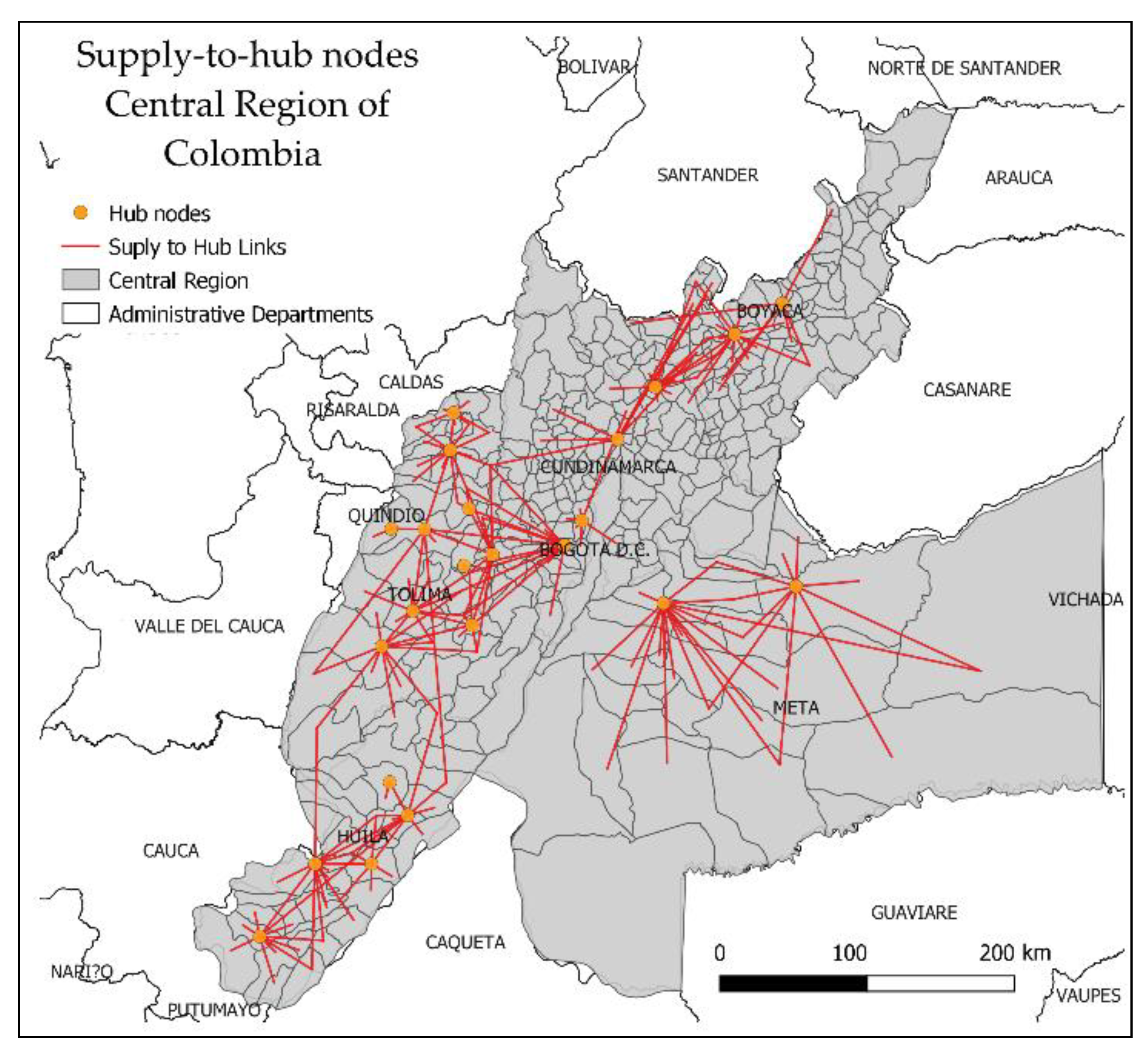
Figure 4 shows the hub locations and their links with the farmers in this baseline. The solid lines are links that account for more than two (2) weekly tons of delivered products.

Figure 5a shows the geographical location of the 23 open hubs and the total tons supplied in the baseline scenario. We can observe that the larger supplied quantities are concentrated to the west of the central region where more and larger hubs are open. In this part of the central region, most hubs operate at full capacity. This area concentrates the larger portion of total agricultural production (see Figure 1b). Additionally, the population of the cities in this area, indicated in Figure 1a, and of its neighbors make the area attractive for the food hub business. The largest open hubs are located in the provincial capital cities of Villavicencio (east in the Meta department) and Ibagué (west in the Tolima department) and in the mid-size city of Duitama (Boyacá, north). The first two hubs would be supplied by the rich agricultural regions of the neighbor lowlands whereas the Duitama hub would be supplied by many small farmers of the Andean northern region. The other larger open hubs would be located around the high plain areas of Cundinamarca, the valleys of Huila in the south, and the fertile valleys of the Magdalena river in Tolima.

The participation of the agricultural chains at each hub is shown in Figure 5b. We observe that these results are consistent with the agricultural vocation of each area of the region: Hot and humid flat areas of the western and eastern part of the central region are ideal for rice and other grains, whereas potato, some fruits, and vegetables are mostly cultivated in the mountainous areas of the central region.

We also analyze the quantities delivered to the main cities. Figure 6a shows the quantities from hub-to-demand. As expected, the city that receives the largest quantities is Bogotá, the country capital (about 2800 weekly tons). Considering the hubs in the western part of the central region, we can observe that the proximity to Bogotá clearly facilitates the business activity. Bogotá is by far the largest urban center of the country that also hosts the largest wholesaler (Corabastos) in which, as of today, over 12,000 tons of food are traded daily [1]. Following Bogotá, the other two larger demand points are Medellín (northwest of the region in the Antioquia department) and Cali (west of the region in the Valle del Cauca department). These two cities receive around 400 weekly tons. These cities are out of the Central Region, but their size, population, and proximity with several hubs near the borders of the central region, are a reason for their business. The other smaller cities (Ibagué, Neiva, Villavicencio, Tunja, Cartagena, and Barranquilla) commercialize between 5 and 65 weekly tons. Although, the area around Ibagué in Tolima (west) is a large producer of foods, a large portion of them is delivered to other big cities. In general, Figure 6b indicates that the most traded products are grains, fruits and vegetables (F&V), and “other products”. Potato and plantain chains are smaller chains because they only contain two or three products. Notice that production quantities of these two chains are virtually not delivered to the northern cities of Cartagena and Barranquilla (circles in the upper part of Figure 6b). The cost and profits analysis follows next.

We also compare the baseline in relation of the current situation of no hubs in which products are delivered directly to the cities. We can observe that all transportation and emission costs decrease with the hubs’ network. This is achieved mainly due to reductions in the vehicles’ operation fixed costs and emissions’ costs (up to 95% reduction). This cost savings can be explained as fewer vehicles are required when cargo is consolidated at the hubs. In the scenario of no hubs, the number of vehicles used is approximately 8000 per week, considering that each farmer (or middlemen) travels to the cities in small trucks. With the hubs’ network, the number of vehicles required to transport food is around 800, which represents a 90% reduction. The additional benefit is that fewer vehicles also reduce the total emissions of CO2, improving the carbon print. Figure 7 presents this comparison.

5.3. Variation in the Exponent $\gamma$ and in Hubs’ Costs

Table 7. Summary of the results in 14 scenarios with variation on the baseline scenario.

Scenario	$\mathit{\gamma }$	Hub Fixed Costs Variation	Average Quantities Handled by Hubs (Tons)	Total Quantities (Weekly Tons)	Number of Hubs	Net Profit
Baseline	2.0	0%	77	8866	23	951
1	0.1	−20%	58	4601	16	413
2	0.1	0%	60	4486	15	413
3	0.1	+20%	69	4157	12	372
4	0.5	−20%	54	4866	18	440
5	0.5	0%	58	4661	16	435
6	0.5	+20%	67	4328	13	389
7	1	−20%	54	5446	20	512
8	1	0%	58	5237	18	506
9	1	+20%	65	4519	14	379
10	2	−20%	77	8866	23	982
11	2	+20%	79	8695	22	895
12	3	−20%	84	10,100	24	1293
13	3	0%	81	10,089	25	1201
14	3	+20%	81	10,089	24	1204

shows the results of scenarios presented in Table 6. Analyzing the results, we can observe that with low values of the sensitivity distance exponent $\gamma$, fewer hubs are open as smaller quantities are delivered from farmers to hubs; the opposite is true for larger values of $\gamma$. The differences are important: For $\gamma =0.1$ (low distance attractiveness), the number of open hubs ranged between 12 and 16, whereas for $\gamma =3.0$, the number of hubs ranged between 24 and 25.

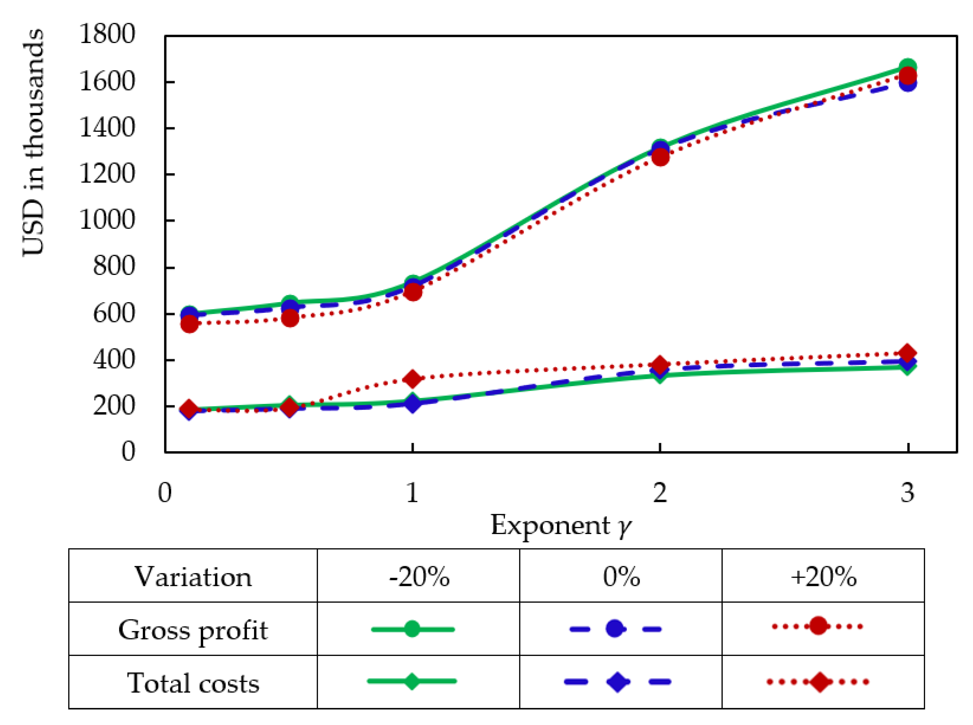
Figure 8 illustrates the effects on the gross profit and the total cost of these parameter combinations. We can notice that the variation in hubs’ costs represents a less significant change in the number of open hubs and on the traded quantities in comparison with changes in the exponent $\gamma$. This behavior corroborates the results shown in Table 7. With values of $\gamma$ less between 0.0 and 1.0, the variations are small; however, if the exponent $\gamma$ is greater than 1.0, the gross profits rise steeply. On the other hand, Figure 8 also shows that net profit in all cases is greater than 0. This means that the hubs’ network might be a cost-effective business for concessionaires.

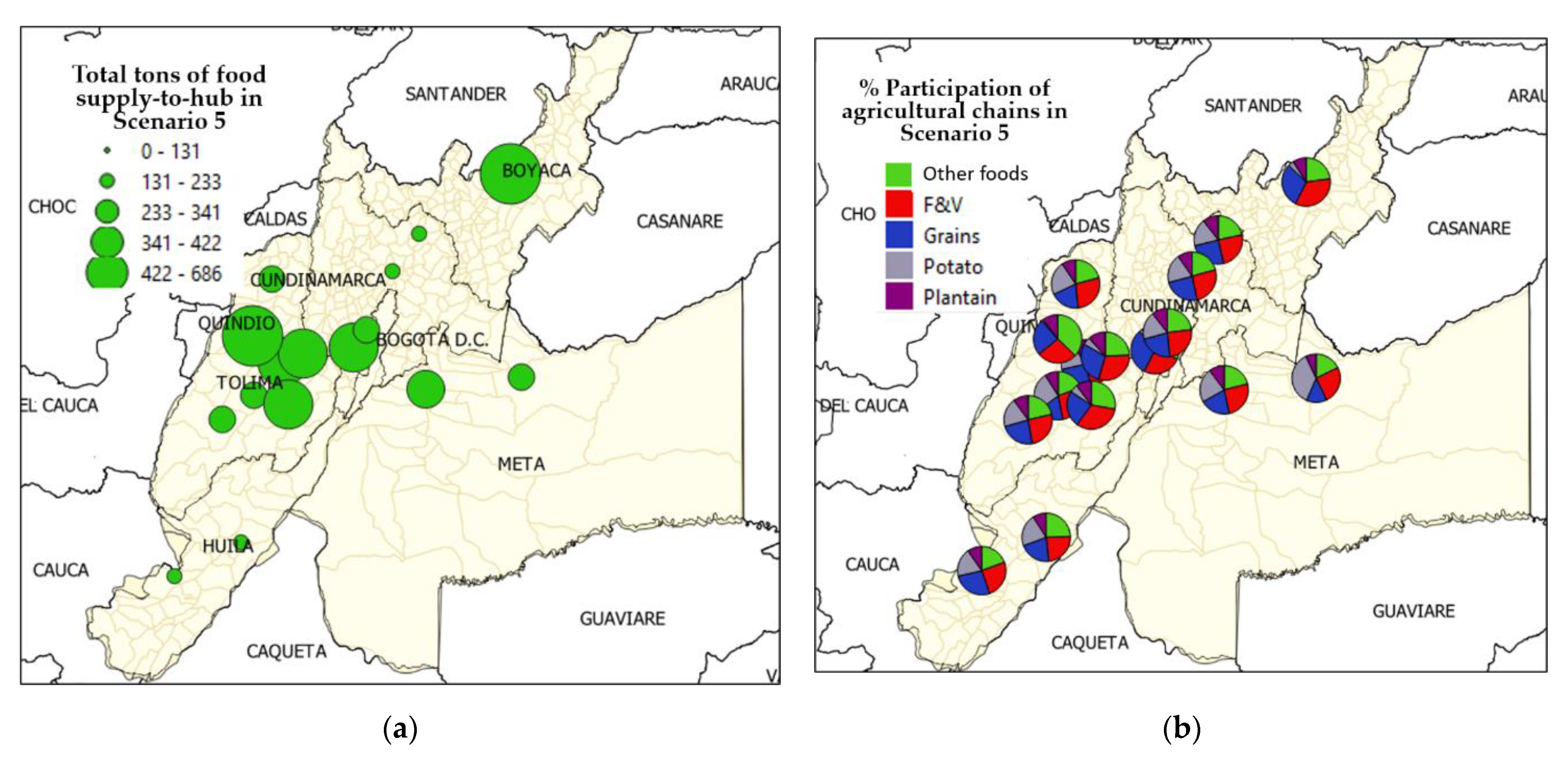
For the purpose of comparison, we selected a scenario with low sensitivity to distance ($\gamma )=0.5$ and 0% fixed cost variation. This is scenario 5 of Table 7. The results are illustrated in Figure 9a. The solution shows that 16 hubs are open, and that the pattern of hub locations is similar to the baseline scenario. However, in most cases, the traded quantities are smaller, as fewer farmers are attracted in this scenario. Only in the case of the Duitama hub (the large circle in the Boyacá department), the quantities handled are similar in comparison with the baseline. The explanation is that the strategic location and the lack of competitors of this hub make it the only trading option in this region for the small and medium size farmers of northern Boyacá. In the department of Huila in this scenario, only two (as opposed to five in the baseline) hubs are open, and the corresponding trading quantities are smaller.

5.4. Results of Capacity Variations

This section shows the results of the experiments with the variation in hubs’ capacity in comparison with the baseline scenario.

Table 8. Summary of results of hubs’ capacity variations. The weekly gross profit, total costs, and net profit are presented in thousands of USD. The letter × represents the capacity’s initial value.

Increase in Hubs’ Capacity	Gross Profit	Transportation Costs	Emission Costs	Fixed Hubs’ Operation Costs	Net Profit	No Hubs	Total Handled Quantities (tons)
Baseline 1×	1310	198	16	146	950	23	8866
1.5×	1617	232	17	206	1162	21	11,095
2×	1884	265	19	274	1326	21	13,255
3×	2244	313	21	412	1498	21	16,488

shows these results.

As expected, the greater the capacity, the greater the quantities are traded, and the greater the net profits are. In the three new scenarios, the number of open hubs is 21. The trend, however, is of diminishing returns. Doubling the capacity in relation to the baseline produces a net profit of USD 1,162,000 (39% increase) whereas tripling the capacity produces a net profit of USD 1,498,000 (57% increase). In terms of quantities, the relation with the capacity increments is approximately linear: An addition of one percentage point in capacity represents an increase of approximately 37 handled tons. The fixed operation costs also increase in a linear fashion in relation to the baseline. An increment of one percentage point in capacity represents on average an increase of around USD 1360 in fixed costs.

We can also observe that the transportation costs also increase compared to the baseline as hubs handle larger quantities of products, which in turn require more trucks. However, the transportation costs do not increase that steeply: For example, tripling the hubs’ capacity results in an increase of 58% in the transportation cost. This implies that the greater the hubs’ capacity, the better use the vehicles’ capacity. In terms of emission costs, there is a moderate increase. For example, tripling the hub’s capacity increases the emission costs in 23%.

5.5. Results of Margin Variations

The last proposed experiment is the variations in the gross profit margin. As said above, this business is meant not only to be profitable, but also to help farmers to obtain better prices. Thus, a reduction in the hubs’ margin can be translated to the farmers as in [11].

Table 9. Summary of margin variations’ results. The gross profit, total costs, and net profit are presented in thousands of USD per week. The letter × represents the margin’s initial value.

Variation in Margin of Gross Profit	Gross Profit	Transport Costs	Emission Costs	Fixed Operation Costs	Net Profit	No Hubs	Total Handled Quantities (Tons)
Baseline 1×	1310	198	16	146	950	23	8866
0.9×	1147	187	15	134	812	21	8405
0.75×	941	174	13	134	621	21	8405
0.5×	593	138	9	131	315	20	8345

illustrates these results.

We observe that with the reduction in the gross margins, the number of hubs reduces as well. Likewise, the delivered quantities are smaller. The net profit also reduces accordingly. However, analyzing the net profit, even with a 50% gross margin reduction, the profits can be still attractive for concessionaires.

The model shows that a reduction in margins has a moderate impact on the overall logistics operation: Although fewer hubs are open, the reduction in the number of hubs is not significant (23 in the baseline vs. 20 in the 0.5× scenario and a reduction of approximately 500 tons per week or 166 tons/hub-week). A similar analysis can be performed for the transport costs, emissions, and fixed operation costs of the hubs. The greatest impact is on profits: Reducing the margins in 50%, the profits would decrease in around 66% (950,000 vs. 315,000). This situation may be extreme, but shows the potential savings that can be achieved at both ends of the supply chain (farmers and end costumers).

6. Conclusions

The results illustrate many interesting things: First and most noteworthy is that the hub strategy can be a profitable activity if the hubs are put into operation. In the experiments, we varied everything that could reasonably be changed, and even in scenarios with low attractiveness (low quantities handled by the hubs) and low margins, the business was still profitable. For example, in the baseline, the estimate weekly net profit is USD 951,000 which corresponds to an average weekly net profit of around USD 40,000 per hub. The total costs in this baseline scenario, calculated from Figure 5, are USD 360,000. In this case, the weekly net profits are almost three times the total costs. In the extreme case of the lowest value of sensitivity to distance ($\gamma$) and the highest fixed costs, the weekly net profit is USD 372,000 and an average weekly net profit of around USD 31,000 per hub. In terms of factors that affect the profitability, the sensitivity exponent appears to be the most important as illustrated in Figure 8. For instance, keeping the fixed costs variation constant at 0%, we can observe that the weekly net profits ranged from USD 413,000 to USD 1,201,000 (almost three times). It can also be noticed, in the same figure, that varying the fixed costs produced nearly no variations in the gross profits.

Second, as said above, there were scenarios in which the optimal solution resulted in zero (0) open hubs. These were scenarios in which hubs failed to attract farmers (low values of $\gamma \mathrm{and} \delta$). This implies that the private (hub concessionaires) and the public institutions (e.g., RAP-E-) have the challenging task of promoting the usage of the hubs (i.e., increase the values of $\gamma$). This can be done through education and better trading conditions for farmers. This is not easy for people who have been isolated for years and are reluctant to change their culture and traditions. In our point of view, major attractors would be offering (i) better margins in comparison with those of the middlemen, (ii) technical assistance and farm inputs, and (iii) on-the-spot cash payments. The E-choupal initiative [11] is an example of success in the transformation of rural India with these three ideas.

Third, increasing the capacity of the hubs does increase the net profits, but there can be limitations. Although the fixed costs and transportation costs also increase, the larger quantities that these hubs can handle result in greater profits as presented in Section 5. The question is if the hubs’ concessionaires can increase their operation capability. As said above, increasing the capacity can be seen as adding days of operation, which seems plausible. A potential limitation for the extended operation is the availability of trucks. For example, a given truck cannot be used on a daily basis and will only be available at the hub in three to five days, depending on the route.

Lastly, there are difficulties to overcome before the successful implementation of a model like this: First, middlemen would not easily give up their business. Intermediation in Colombia is a big business, and a big hub competitor would not be welcome. A potential strategy is creating middlemen memberships to the hub concessionaires and therefore they would participate of the profits. Second, if the hubs are too distant from the farmers, hubs would be of no use. In this sense, hubs would only be useful for farmers located in relatively well-connected areas, and those farmers in remote areas would still rely on middlemen. Finally, the investment to refurbish the hubs can be significant, and at the present pandemic time, the central government has other priorities and limited budget to execute projects like this.

7. Final Thoughts and Further Research

This paper has presented a mathematical model for food hub locations in the central region of Colombia. The model considers the special characteristics of the supply and distribution of the fresh food supply chain in the region, namely dispersed farmers in the countryside that make choices as to where they sell their products and food hubs that distribute such products to urban centers. To the best of our knowledge, this problem has not been studied in the literature. This problem is of special relevance because public institutions in Colombia, responsible for the design and implementation of the master plans for food supply and food security, are closely following the results of this model.

This research uses extensions and adaptations of several competitive hub and facility location formulations to create a realistic model that can be used as a first input for policy making. The results show that the model can be viable and sustainable in the long term under several conditions, as described throughout the paper. This proposed model, of realistic size, was tested with real data. Extensive experiments suggest that the ability of the food concessionaires to attract farmers is the main success factor for the business model.

Based on the results presented throughout this paper, managers and decision makers of the central region can devise an articulated set of tax and legal incentives to attract private investment for the creation and/or strengthening of logistics strategies with technical and operational capacities to efficiently deal with the operation of the hubs. At the same time, education and sensibilization campaigns must be carried out with all stakeholders in order to guarantee a smooth operation of the hub network.

Future research will be carried out with extensions such as logistic regression models that capture additional decision factors such as prices and social network, to name a few. Multi-objective extensions considering environmental factors are also foreseen.